A Short Travel for Neutrinos in Large Extra Dimensions
Abstract
Neutrino oscillations successfully explain the flavor transitions observed in neutrinos produced in natural sources like the center of the sun and the earth atmosphere, and also from man-made sources like reactors and accelerators. These oscillations are driven by two mass-squared differences, solar and atmospheric, at the sub-eV scale. However, longstanding anomalies at short-baselines might imply the existence of new oscillation frequencies at the eV-scale and the possibility of this sterile state(s) to mix with the three active neutrinos. One of the many future neutrino programs that are expected to provide a final word on this issue is the Short-Baseline Neutrino Program (SBN) at FERMILAB. In this letter, we consider a specific model of Large Extra Dimensions (LED) which provides interesting signatures of oscillation of extra sterile states. We started re-creating sensitivity analyses for sterile neutrinos in the 3+1 scenario, previously done by the SBN collaboration, by simulating neutrino events in the three SBN detectors from both muon neutrino disappearance and electron neutrino appearance. Then, we implemented neutrino oscillations as predicted in the LED model and also we have performed sensitivity analysis to the LED parameters. Finally, we studied the SBN power of discriminating between the two models, the 3+1 and the LED. We have found that SBN is sensitive to the oscillations predicted in the LED model and have the potential to constrain the LED parameter space better than any other oscillation experiment, for . In case SBN observes a departure from the three active neutrino framework, it also has the power of discriminating between sterile oscillations predicted in the 3+1 framework and the LED ones.
Keywords
neutrino oscillation, large extra dimension, short-baseline1 Introduction
Our knowledge of the three neutrino oscillation paradigm has substantially improved in the last decade mainly thanks to the reactor and accelerator-based experiments [1, 2]. Nowadays, the neutrino oscillation parameters have been measured with certain precision [3, 4], except for the Dirac phase encoding the possibility that leptons violate the charge-parity (CP) symmetry. In this so-called three active neutrino framework, the neutrino mass ordering, whether the third mass eigenstate is the upper (normal ordering) or the lower (inverted ordering) of the three states, is also unknown. Future neutrino oscillation experiments are expected to resolve both important missing pieces and also to improve over the current precision of the neutrino oscillation parameters. In particular, there is a quest for establishing if the atmospheric mixing angle is maximal, and if not, what would be its correct octant. Besides providing information on the unknowns, in the precision era, new physics signals might emerge as subleading effects of the three neutrino paradigm or as a new oscillation phase(s). This last scenario is mainly motivated by results of short-baseline experiments [5, 6, 7, 8] which call for a new neutrino flavor state that has to be sterile, i.e. it can not interact with the Standard Model gauge bosons. So far, there is no indication of a new oscillation phase and running experiments have constrained a large part of the parameter space, at least in the economical oscillation framework [9, 10, 11, 12, 13, 14, 15, 16]. Several efforts are devoted to discover a sterile oscillation at the eV mass scale or to completely rule out this hypothesis. For instance, at FERMILAB, there is a Short-Baseline Neutrino Oscillation Program (SBN) [17], which is expected to provide a definitive answer to this matter. However, there are several beyond the standard three-neutrino oscillation scenarios, which might be considered as a the subleading effect, that can be probed in future long and short-baseline neutrino experiments. Here we focus on Large Extra Dimensions (LED) and the possibility that its signals be differentiated from the sterile hypothesis at the SBN program. Other proposals can be tested in SBN facility for instance the search for multiple sterile states [18, 19, 20] and MeV-scale sterile decay [21, 22, 23].
Initially, the main motivation for introducing extra space-time dimensions was to lower high energy scales, as for instance the GUT [24, 25] or the Planck scale, even to the TeV energy scale [26, 27, 28]. This appeared as an alternative to the usual seesaw mechanism that in its natural form calls for a high energy scale to suppress the active neutrino masses. Since right-handed neutrinos are singlets under the Standard Model (SM) gauge group, they are one of the candidates that can experience extra space-time dimensions and therefore collect an infinite number of Kaluza-Klein excitations [29, 30]. The other SM fermions are restricted to a brane and therefore experiencing four dimensions only. In this way, the Yukawa couplings between the right-handed neutrinos and the active ones are suppressed by the volume factor after compactification of the extra dimensions. In this context, neutrinos acquire a Dirac mass that is naturally small, however, other alternatives violating lepton number are possible [29]. It is phenomenological appealing to considered an asymmetric case where one of the extra dimensions is ‘large’ respect to the others, effectively reducing the problem to be five dimensional [30, 29, 31]. In this letter, we consider the model for Large Extra Dimensions (LED) from Ref. [31] (which is based on previous works in Refs. [29, 30, 32]), and recently considered in the context of DUNE in Ref. [33], with three bulk neutrinos (experiencing extra space-time dimensions) coupled to the three active brane neutrinos.
In this letter, we consider neutrino oscillations within the LED model with three bulk neutrinos coupled to the three active brane neutrinos, which effectively act as a large number of sterile neutrinos in contrast to the usual oscillation of light sterile neutrinos at the eV energy scale. Our goal is to establish the sensitivity of the SBN program to neutrino oscillations in the LED model. This letter is organized in the following way. We first introduce the LED formalism in Section 2. The SBN program and the experimental details used in our numerical simulations are condensed in Section 3. Our results are presented in Section 4. Finally, we conclude and summarize in Section 5.
2 Formalism
In general, it is assumed the right-handed neutrino (bulk fermions [31]) can propagate in more than four dimensions while the left-handed neutrino , and the SM Higgs , are confined to the four-dimensional brane. It is also assumed that one of the extra space-time dimensions is larger than the others so that effectively it is enough to consider five dimensions in total. A Dirac fermion in five dimensions can be decomposed into two component spinors (Weyl fermions), and and after the extra dimension is compactified a natural coupling with emerges [29] and, as a result, Dirac neutrino masses are obtained [29, 30, 32, 31]. Along this letter we follow the model with three bulk neutrinos coupled via Yukawa couplings to the three active brane neutrinos, the so-called model in Ref. [31]. Other formulations for large extra dimension models are possible as described in Ref. [34].
The action in the model is given by:
| (1) |
where is the coordinate of the extra compactified dimension, are the five-dimensional Dirac matrices for , and the Yukawa couplings. To compactify the action in Eq. (1) one need to expand the the five-dimensional Weyl fields in Kaluza-Klein (KK) modes (with ) and also to impose suitable periodic boundary conditions [29]. It is convenient to define the following linear combinations:
| (2) |
for , and also . Therefore, after electroweak symmetry breaking, the Lagrangian mass terms that results from Eq. (1) are given by:
| (3) |
Where is the Dirac mass matrix that is proportional to the Yukawa couplings and can be written in terms of the fundamental mass scales of the theory [29, 31], and is the compactification radius. It is useful to consider a basis in which the Dirac mass is diagonal [31] , by defining pseudo mass eigenstates [35], such that the mass Lagrangian in Eq. (3) can be written where is the infinite-dimensional matrix given by [30, 31]:
| (4) |
To find the neutrino masses and the relevant unitary matrices that relate the mass eigenstates with the pseudo eigenstates , , one needs to perform the bi-diagonalization . However, since we are mostly interested in the relation of the active brane neutrino states with the mass eigenstates, it is enough to consider only the left matrices and . is obtained from the diagonalization of the Hermitian matrix while is the unitary matrix involved in the diagonalization.
Effectively the active neutrino flavor states, can be finally written in terms of the mass eigenstates (as composed of the KK -modes of the fermion field), as follows:
| (5) |
where is the amplitude in the LED case. We recover the usual three-neutrino case when .
Formally, the mass eigenvalues and the eigenvectors of in Eq. (4) are obtained from the diagonalization of the matrix by assuming a maximum integer value for the KK-modes and then taking the limit [29, 30]. The matrix in Eq. (5) is explicitly given by:
| (6) |
where the neutrino mass eigenstates are equal to and therefore each one of them is composed of -KK modes. in Eq. (6) corresponds to the eigenvalues of the full neutrino mass matrix and can be calculated from the following transcendental equation:
| (7) |
and the roots are constrained such that they belong to the range [29]. In order to make a physical sense of the formalism, one should assume that the most active state is obtained for . Additionally, if we go to the limit then , and following Eq. (6) , therefore recovering the standard result where is the lepton mixing matrix that is usually parametrized by three rotations 11 1 The three rotations are in general complex, accounting for the three physical CP phases. However, neutrino oscillations are insensitive to the two Majorana phases, and therefore, only sensitive to the Dirac CP phase. In this case the more used parametrization is written as two real rotations plus a complex one., through the three mixing angles , and the Dirac CP phase .
Assuming the mostly active mass state is related with the lightest mass state in the KK-tower implies a relation between the eigenvalues of this LED framework, obtained by Eq. (7), with the square mass differences obtained in the three-neutrino case. This relation can be written as:
| (8) |
with is the solar () and the atmospheric () squared mass differences. Therefore, the existing values on the squared mass differences of the active neutrino mass eigenstates , Ref. [36, 4], constrain the parameter space of the LED model. Thus, a good strategy is to use this information before scanning the parameter space. Basically, , i=1,2,3 are fixed by the in Eq. (7), and using Eq. (8) for k=2,3 we got a constrain between , and [37]. With these constraints, we have now only two independent parameters and that we will rename from now on as for normal mass ordering. Similarly, one can follow the same procedure for the inverted mass ordering, and this case the two independent parameters are and . In the cases where the condition in Eq. (8) is not fulfilled by the combination, we quoted the excluded region as excluded by squared mass differences constraints. We will comeback to this point in Section 3.
In the LED framework the neutrino mixing matrix , as defined in Eq. (5), is in general different to the standard three neutrino mixing matrix . To avoid spoiling the neutrino oscillations observations, condensed in part as constraints on the mixing angles () in scenario of three-neutrino scheme (with values in Ref. [3, 36, 4]), the mixing angles in the LED framework have to be redefine. Following the procedure from Ref. [33] we have defined new mixing angles () in the LED scenario such that the lowest mass state in KK tower, , have the amplitude equal to the numerical value of : . From this relation we can get the mixing angles in the LED framework, , related with the solar and atmospheric mixing angles, . Explicitly we have using the elements of mixing matrix , and
| (9) |
From now on, the mixing angles in the LED formalism are given by the values in Eq. (9). For some values of and the value can be smaller than the numerator in Eq. (9) such that and thus unphysical. In this way, values of and that results in this unphysical will be disregarded and we have quoted them as excluded by mixing angle constraints. We will comeback to this point in Section 3.
3 Simulation
In this section, we describe the experimental set-up and our working assumptions that we followed in the sensitivity analyses presented in Section 4. The SBN experimental proposal will align three liquid argon detectors in the central axis of the Booster Neutrino Beam (BNB), located at FERMILAB [17]. Table 1 gives the SBN detector names, active masses, locations, and protons on target POT. We computed the expected number of events of SBN facility by implementing the detectors in the GLoBES [38, 39] c-library, following the proposal description. The flux information for both neutrino and anti-neutrino modes was taken from Ref. [40], and the neutrino-argon cross section was taken from inputs to GLoBES prepared for Deep Underground Neutrino Experiment (DUNE) simulation [41], with the cross section inputs, originally generated using GENIE 2.8.4 [42].
Detector Active Mass Distance from BNB target POT Lar1-ND 112 t 110 m MicroBooNE 89 t 470 m ICARUS-T600 476 t 600 m Electron Neutrino Appearance Channel Muon Neutrino Disappearance Channel Energy Bin Size (GeV) Energy Range (GeV) Energy Bin Size (GeV) Energy Range (GeV) 0.15 0.2-1.10 0.10 0.2-0.4 0.20 1.10-1.50 0.05 0.4-1.0 0.25 1.50-2.00 0.25 1.0-1.5 1.00 2.00-3.00 0.50 1.5-3.0
The SBN facility will search for oscillations in two channels: 1) electron neutrino appearance from muon neutrino conversion () and 2) muon neutrino disappearance () from muon neutrino survival. We considered a Gaussian detector energy resolution function with a width of for muons and for electrons, according to Ref. [20]. The energy range for the neutrino event reconstruction extends from 0.2 GeV to 3 GeV where each channel has different bin widths, as described in the Table 1. We simulated three years of operation for the neutrino beam in Lar1-ND and ICARUS-T600 detectors and six years in MicroBooNE detector. It is important to emphasize that the detectors do not make a distinction between neutrinos and anti-neutrinos, so neutrinos and anti-neutrinos events are added in our simulations. After event reconstruction, we included an efficiency factor for each channel in order to mimic event rates from collaboration proposal [17].
In the presence of LED, the relations in Eq. (8) and Eq. (9) gives the squared mass differences and the mixing angles in terms of the standard oscillation parameters. When simulating neutrino event rates, to perform the different studies along this letter, we used the best-fit values for the oscillation parameters in the standard three-neutrino framework presented in Nu-Fit 3.2 (2018) [36, 4]. The LED parameters are the lightest neutrino mass (for normal ordering while for inverted ordering ) and the radius of extra dimension .


In Figure 1 the behavior of the oscillation probability for different and values is shown, considering an of km/GeV in both appearance and disappearance channels for both normal and inverted neutrino mass ordering. The value was calculated using the ICARUS baseline km and the energy GeV, which corresponds to the region in the neutrino energy spectrum where most of the events are expected [17]. We noticed that for all LED parameters in the plane, the appearance probability is not larger than 10-3 and almost all survival probability is larger than 0.9. The gray shaded region is excluded by neutrino oscillation data, with the relations Eq. (8) and Eq. (9), as described in Section 2.
In the following, we assume forward horn current (FHC) beam mode and we defined signal and background for each one of the SBN oscillation channels as follows:
- •
Muon neutrino disappearance channel:
- 1.
Signal: Survival of muon neutrinos () from the beam which interact with liquid argon through weak charged-current (CC) producing muons in the detectors.
- 2.
Background: The only background contribution considered by the collaboration comes from neutral-current (NC) charged pion production, where the pion produced in the BNB target interacts with argon and can be mistaken for a muon [17]. This contribution is small due to the track cutting imposed in the event selections and we did not consider it in our simulations.
- 1.
- •
Electron neutrino appearance channel:
- 1.
Signal: electron neutrinos coming from muon neutrino conversion () which interacts through CC producing electrons in the detectors.
- 2.
Background: The main background contribution comes from the survival of intrinsic electron neutrinos () in the beam, beam contamination. We also considered muons (muon neutrinos from the CC interaction), which can be mistaken for electrons. NC photon emission, cosmic particles and dirty events were not considered in our simulation, which corresponds to a background reduction of for Lar1-ND, for MicroBooNE and for ICARUS-T600, respect to the total number of background events expected by the collaboration in the electron neutrino channel [17].
- 1.
The information on the neutrino fluxes, neutrino cross section, energy resolution of leptons and backgrounds used in the analysis were compiled using the AEDL format (to be used with the GLOBES c-library), in order to perform the different sensitivity analyses of SBN program at FERMILAB. These files are available under request following Ref. [43].
Since one of the main goals of the SBN program is to detect or rule out sterile neutrino oscillations, we introduce the generalities of the case right now. Later, we will not only take it as a reference but also we will quantify the discrimination power of the SBN program between the two models, the and the LED. Several neutrino experiments have performed a sensitivity analysis in the specific scenario of the so-called 3+1 model, where one sterile neutrino is added to the three active neutrino framework. In this 3+1 framework, active and sterile neutrinos mix and three new oscillation frequencies appear, thanks to the four mass eigenstates, which can be written in terms of only , the solar, and the atmospheric splittings. The additional mass eigenstate is the source of short-baseline oscillations mainly driven by the square mass difference , and the effective amplitudes and defined by the elements of the lepton mixing matrix. We have successfully reproduced the results of the SBN experimental proposal regarding the sensitivities to the sterile parameters by the implementation of the muon disappearance and electron appearance oscillation channels. These sensitivities will be considered and shown in Section 4.
In the following sections, we present results based on different sensitivity analysis, using both muon and electron appearance channels, unless otherwise stated. We studied three cases assuming a given event energy spectrum for ‘data’ (or ‘true’ events) and we have performed a hypothesis testing based on a Poisson function for the different models: 1) ‘data’ simulated assuming an energy spectrum defined by the three-neutrino case an testing the LED hypothesis, i.e., the usual sensitivity analysis, 2) ‘data’ simulated assuming an energy spectrum distributed with the LED model and testing the standard oscillation scenario. Here we investigated the SBN potential of measuring the LED parameters and . Finally, 3) ‘data’ simulated assuming an energy spectrum distributed with the 3+1 model, where we evaluated the discrimination power of SBN to distinguish LED hypothesis from other models accommodating light sterile neutrino oscillations. We also performed sensitivity calculations for the 3+1 model in appearance and disappearance channels in order to explore relations between LED and 3+1 signatures. The results are shown in the next section.
4 Results
For the sensitivity analysis, total normalization errors in signal and background were set to , and all parameters that were not shown in the plots were fixed to their best-fit values. We tested that our sensitivity results are independent of the value. For simplicity, we set for normal ordering and for inverted ordering, according to Ref. [4].


Figure 2 shows SBN sensitivity limit with of confidence level (C.L.) in the green curve for normal (left panel) and inverted ordering (right panel), compared with other limits: Sensitivity limits at 95 % of C. L. for DUNE experiment (black-dashed curve) presented in Ref. [33], as well as ICECUBE-40 data and ICECUBE-79 data (dot-dashed magenta and blue curves, respectively) from Ref. [44], and the combined analysis of T2K and Daya Bay data (dot-dashed gold curve) presented in Ref. [45] are shown. The preferred region (in pink) at 95% C. L. by Gallium and Reactor anti-neutrino experiments from the analysis in Ref. [46] is also included. Finally, sensitivity limits for KATRIN at C. L. (dashed brown curve) due to kinematic limits in beta decay estimated in Ref. [37] are shown. The gray shaded regions are the parameters excluded by measurements of square mass differences and (light gray) and of mixing angles , and (dark gray). It is important to mention that excluded region due to mixing angle measurements also covers excluded region due to square mass differences. An additional constrain to the LED parameters comes from MINOS analysis in Ref. [47] where a similar restriction curve to the one from ICECUBE was obtained. When , MINOS constrains m (or eV) for normal ordering.
We can see that the SBN program is sensitive to the LED parameters and this sensitivity is very competitive, respect to other facilities shown in the plot. This happens specifically for the lower region and particularly for normal ordering. Comparing with the constraints from other experiments, the SBN sensitivity for LED mechanism is the better than any other constraints in the region when for normal ordering, and in this region, the maximum sensitivity of our analysis for is better than any other oscillation experiment which we trace to the fact that we are testing LED in a short-baseline experiment for the first time, all other sensitivity results corresponds to long-baseline experiments. With respect to the reactor anomaly allowed region, the SBN program has the potential to ruled out completely this anomaly for any value of . For higher values of , the DUNE experiment [33] have the potential to exclude the reactor anomaly allowed region, complementing SBN.
4.1 Sensitivity to a non-zero LED oscillation effect on SBN
In order to investigate the potential of SBN to measure the LED parameters, neutrino events were calculated in the same fashion than for the previous sensitivity analysis, but assuming now the LED model with and as the ‘true’ values, and testing the LED scenario. All the standard oscillation parameters (which are included in the LED parameters) were fixed to their best-fit values from Refs. [36, 4] as described in Section 2. Figure 3 shows the allowed regions consistent with the computed events with the true value (black dot) at of C.L. (blue curve), of C.L. (orange curve) and of C.L. (purple curve) for both normal ordering (left panel) and inverted ordering (right panel).
We also included in Figure 3 the sensitivity result obtained in Figure 2 (dashed green line), which we called Blind Region, i.e., the region that agrees with the standard three-neutrino scenario, being in this way, ‘blind’ to LED effects. Any point inside the Blind Region will have a null result either for the muon disappearance channel or for the electron neutrino appearance channel. The Ch. Blind Region presented in Figure 3 (dashed brown line) is the result of the sensitivity analysis performed only with the computed events from electron neutrino appearance channel. Any point inside the Ch. Blind Region will have a null result for the electron neutrino appearance channel. The ‘true’ LED parameters were chosen around the Ch. Blind Region, but outside the Blind Region for both mass ordering.
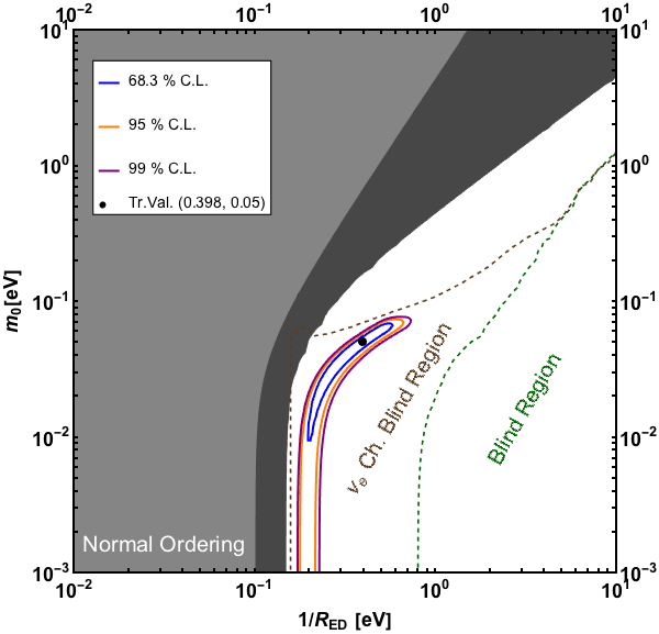
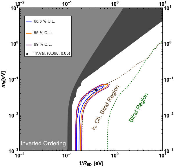
It is worth noticing that since the electron neutrino appearance probability is smaller than for LED, as shown in Figure 1, one might not expect a sensitivity exclusion limit from the appearance channel, i.e., all the obtained sensitivity is shown in Figure 2 would come from the muon disappearance channel. However, when we computed the sensitivity curve only considering electron appearance channel, we obtained the exclusion limit showed in Figure 3 (dashed brown line). In fact, we have a sensitivity curve from electron appearance channel when we consider changes in background profile due to LED effects. The electron neutrino survival probability induced by the LED parameters decreases the intrinsic electron neutrinos from the beam, which is the majority contribution to our background. In other words, we have sensitivity due to the decrease in the number of backgrounds and not by the increase in the signal. A similar effect was found in Ref. [20].
Although not shown in Figure 3, we repeated the same analysis with other LED true values located inside the exclusion region for both electron and muon neutrino channels (outside the Blind Region and the Ch. Blind Region). In this case, we have a non-null result in both muon disappearance and electron neutrino appearance channels, and therefore the LED parameters that explain this results are unique. As a consequence of this, and due to the logarithmic scale in the plot, we obtained small and concentrated regions around the chosen ‘true’ values, which results in a precision of SBN experiment to the LED parameters below 1%.
4.2 3+1 scenario at SBN: sensitivity and accuracy of the measurement
In the standard three-neutrino scenario, we expect no oscillations in SBN due to its short-baseline and the energies considered. Now, if SBN ‘sees’ an oscillation, it will corresponds to a beyond the standard three-neutrino scenario signal that might be interpreted as an sterile neutrino oscillation. In the 3+1 scenario, the neutrino probabilities for short-baseline distances are given by [48]:
| (10) | ||||
| (11) | ||||
| (12) |
where , with and are the oscillation amplitudes, defined by the elements of the generalized PMNS matrix elements and , and is the squared mass difference between the fourth mass state (which is made majority by the sterile component of neutrino flavor basis) and the first mass state . The probabilities in Eqs. (10), (11), (12) at short-baselines depend on the three parameters [49].


We now test the two following cases in the 3+1 scenario:
- 1.
Assuming the ‘true’ event energy distribution as compatible with the three-neutrino scenario and testing the 3+1 model. This gives the sensitivity of SBN to the 3+1 scenario that can be seen in Figure 4. Exclusion regions are to the right of the black curves for both appearance (right panel) and disappearance (left panel) channels. We have a very good agreement with the SBN sensitivity, comparing the blue and solid curves in Figure 4.
- 2.
Assuming as the ‘true’ event energy distribution as compatible with the 3+1 scenario and testing the 3+1 model. This will give the accuracy of SBN facility to the parameters of the 3+1 scenario that can be seen in Figure 5. For illustration purposes, we show the sensitivity as dashed black curves for the 3+1 model at the SBN from Figure 4. The allowed regions assuming the ‘true’ 3+1 parameters , and and also fitting 3+1 hypothesis. Notice that SBN is very sensitive to the square mass difference around and the precision that we can get for this value are very good and below 1%. Even though not shown in the figure, large values of and gets more precise determined than the lower values shown in the plot. The fast oscillations eV2 were handled assuming a low-pass filter in our analysis using GLoBES 3.2.17 [38, 39], otherwise we will have spurious results in our sensitivity for 3+1 model.


4.3 Discrimination power between LED scenario and the 3+1 scenario
One question that remains is, in the case SBN finds a departure from the three neutrino framework, is it possible to identify which of the two scenarios analyzed in this letter would be responsible for the new signal (assuming is not something else)? In the following, we analyze the discrimination power of the SBN experiment comparing both the LED and the 3+1 scenarios. Regarding the 3+1 fit to the LED scenario, we calculated events with the ‘true’ LED parameters and assuming normal ordering. With this ‘true’ events, both appearance and disappearance channels were fitted separately, fixing the parameters not shown in the plots. Figure 6 shows the result of the fit in the disappearance channel (left panel) with allowed curves of of C.L. (blue), of C.L. (orange) and of C.L. (purple). The number of degrees of freedom (d.o.f.) was equal to (19 energy bins minus 2 free parameters). The best-fit of the test values is represented in the black dot and has values of and . We have not found a good fit, where for the best-fit point, giving more than 2 of deviation between the two models.


We have also checked that when using the new set of parameters and for the muon disappearance case, we have obtained a for the best-fit (of the test values) point, implying a bad fit. This result can be explained due to the fact that for some values of the LED parameters, as in this case, more sterile states start to contribute in the oscillation probability and the 3+1 model cannot emulate the LED model.
Following a similar procedure, this time fitting the LED model for some ‘true’ values for the 3+1 parameters, we could not obtain good fits. The analysis is shown in the right panel of Figure 6. In fact, if we consider the amplitude and the same eV2, the allowed regions would be almost entire inside the Blind Region (bottom-right part from the dashed green curve in the right panel of Figure 6). From this analysis, we obtained the value . We also considered the case of larger mixing with true values and eV2 and we obtained the value for the best-fit point.
In the case of the electron neutrino appearance channel, we repeated the same procedure done for the muon channel: we calculated events for a given ‘true’ values for the LED parameters and we fitted the electron neutrino appearance parameters in the 3+1 model. The summary of the results are the following:
- •
For eV and eV, the best-fit and the allowed regions were located outside the Sensitivity Region with the value for the best-fit point, implying a very poor fit.
- •
For eV and eV, the best-fit and allowed regions were located outside the sensitivity region, with for the best-fit point, implying a very poor fit.
The previous results (for the electron appearance case) were somehow expected since we could only obtain LED sensitivity from electron neutrino channel in Figure 3 with effects of the LED parameters in the background. Then, we should not expect that the signal of the electron neutrino conversion can be fitted with the 3+1 parameters. In other words, evidence of electron appearance in short-baseline experiments would be inconsistent with LED hypothesis. Similar conclusion was made in Ref. [34].
Disappearance Appearance LED LED 3+1 True: (0.05 eV, 0.398 eV) True: (0.05 eV, 0.398 eV) best fit test Values: (0.1, 0.5 eV2) - 8 78 3+1 True: (0.316 eV, 1 eV) True: (0.316 eV, 1 eV) - - 104 538 3+1 3+1 LED True: (0.1, 0.5 eV2) best fir test values: (0.017 eV, 0.22 eV) * 6.8 LED True: (0.01, 0.5 eV2) - * 187 LED True: (0.1, 3 eV2) - * 149 ( - ) Best-Fit Test Value is outside Exclusion Region, ( * ) LED does not expect positive signal of appearance in SBN.
The right panel of Figure 6 also shows the LED fit for a given set of ‘true’ parameters of the model considering only muon disappearance. We fixed the 3+1 parameters and eV2 and fitted the LED parameters for normal ordering. The allowed curves corresponds to the of C.L. (blue), of C.L. (orange) and of C.L. (purple). The best-fit point obtained is eV and eV. Following the same procedure, we found for the best-fit point.
As we discussed in Section 4.1, with information of the electron neutrino appearance channel (and not the muon disappearance) one can discriminate the LED scenario from the standard three-neutrino case only if changes in the background (i.e. the electron neutrino disappearance from the intrinsic of the beam) are considered. In this way, LED is not contributing to the signal ( conversion) in the electron neutrino channel. Therefore, when regarding the LED fit under 3+1 scenario on these conditions, we would not expect to accommodate LED parameters for any set of ‘true’ parameters of the model considering only the signal of electron neutrino appearance channel.
Finally, all the results obtained for the discrimination power of LED and the 3+1 model are summarized in Table 2.
5 Summary and conclusions
In the dawn of the new era of high precision neutrinos experiments, the search for Beyond Standard Model (BSM) physics will bring an understanding of the mechanism beyond neutrino masses and neutrino mixing. The possibility to have in Nature the presence of large extra dimension is intriguing and it has several consequences for the phenomenology of neutrino physics, such as the existence of infinite tower of Kaluza-Klein states of sterile neutrinos. The Short-Baseline Neutrino Program SBN at FERMILAB will fully test the presence of large extra dimension (LED) in neutrino oscillations.
We have developed GLoBES simulation files [43] that include the three detectors at SBN facility where information of the two main channels of SBN program, the muon neutrino disappearance channel and the electron neutrino appearance channel, are included. In the paradigm of three neutrino oscillation, we expect to see no oscillation in any of SBN detectors. With the assumption that we measure no oscillations in any of SBN detectors, we can put bounds on the LED scenario. In the LED scenario, the non-standard oscillations are accounted for with two parameters, the lightest Dirac neutrino mass and the radius of large extra dimension . We have shown in Figure 1 the regions with sizable muon neutrino disappearance probability and electron neutrino appearance probability in the presence of LED, for either normal or inverted hierarchy of active states. The typical values that we can test are and for a km/GeV.
We showed in Figure 2 the sensitivity plot for the LED scenario that is the main result of this work, based on the simulation details described in Section 3. The solid green curve is the sensitivity of LED scenario, the other dashed curves are the constraints/sensitivities from other experiments for LED scenario and the pink region is the allowed region to explain the reactor neutrino anomaly. We notice that SBN sensitivity curve has, for normal ordering, the strongest bound for almost all parameter region, with exception of the values of eV and eV, for both orderings. From Figure 2, we have learned that all sensitivity to LED scenario came from the muon disappearance channel and that electron neutrino appearance channel plays a marginal role.
Any positive signal of a neutrino oscillation in the SBN facility will be a departure of the present three neutrino paradigm. The main goal of the SBN facility is to test the hint of neutrino oscillation from LSND, Mini-Boone and reactor anomaly. This hint is more usually discussed in the context of the 3+1 scenario with one additional sterile neutrino. Then, we first reproduced the sensitivity region for both channels considered in this letter, under the 3+1 framework with the assumptions described in detail in Section 3. Then, we computed the sensitivity region and compared it with the official sensitivity region of the SBN proposal, reaching a good agreement as shown in Figure 4. In Figure 5, we showed the precision that we can have for a given choice of the parameters in a true 3+1 oscillation scenario. We found that the two channels provide sufficient information to get a few percent of accuracy in the oscillation parameters.
Finally, the remaining question of the power discrimination of the SBN facility: Can the SBN be able to discriminate different physics scenarios when it has a clear departure from the three-neutrino paradigm in the data?, was answered. Table 2 summarizes our results. It is possible to discriminate between both models at . The worst scenario was shown in Figure 6, where we get a discrimination using the muon disappearance channel only. For other choices of parameters, as detailed in Table 2, we can easily discriminate the source of new physics in the SBN experiment, the large extra dimension or the 3+1 scenario.
Acknowledgements.
G.V.S is thankful for the support of FAPESP funding Grant No. 2016/00272-9 and No. 2017/12904-2. G.V.S. thanks the useful discussions with Pedro Pasquini and André de Gouvêa. D. V. F. is thankful for the support of FAPESP funding Grant No. 2017/01749-6. O.L.G.P. is thankful for the support of FAPESP funding Grant No. 2014/19164-6, No. 2016/08308-2, FAEPEX funding grant No. 519.292, CNPQ research fellowship No. 307269/2013-2 and No. 304715/2016-6.References
- (1) Daya Bay collaboration, F. P. An et al., Measurement of electron antineutrino oscillation based on 1230 days of operation of the Daya Bay experiment, Phys. Rev. D95 (2017) 072006, [1610.04802].
- (2) T2K collaboration, K. Abe et al., Measurement of neutrino and antineutrino oscillations by the T2K experiment including a new additional sample of interactions at the far detector, Phys. Rev. D96 (2017) 092006, [1707.01048].
- (3) P. F. de Salas, D. V. Forero, C. A. Ternes, M. Tortola and J. W. F. Valle, Status of neutrino oscillations 2018: 3 hint for normal mass ordering and improved CP sensitivity, Phys. Lett. B782 (2018) 633–640, [1708.01186].
- (4) I. Esteban, M. C. Gonzalez-Garcia, M. Maltoni, I. Martinez-Soler and T. Schwetz, NuFIT, http://www.nu-fit.org/ .
- (5) LSND collaboration, A. Aguilar-Arevalo et al., Evidence for neutrino oscillations from the observation of anti-neutrino(electron) appearance in a anti-neutrino(muon) beam, Phys. Rev. D64 (2001) 112007, [hep-ex/0104049].
- (6) MiniBooNE collaboration, A. A. Aguilar-Arevalo et al., A Search for electron neutrino appearance at the eV2 scale, Phys. Rev. Lett. 98 (2007) 231801, [0704.1500].
- (7) MiniBooNE collaboration, A. A. Aguilar-Arevalo et al., Event Excess in the MiniBooNE Search for Oscillations, Phys. Rev. Lett. 105 (2010) 181801, [1007.1150].
- (8) MiniBooNE collaboration, A. A. Aguilar-Arevalo et al., Observation of a Significant Excess of Electron-Like Events in the MiniBooNE Short-Baseline Neutrino Experiment, 1805.12028.
- (9) Super-Kamiokande collaboration, K. Abe et al., Limits on sterile neutrino mixing using atmospheric neutrinos in Super-Kamiokande, Phys. Rev. D91 (2015) 052019, [1410.2008].
- (10) MINOS collaboration, P. Adamson et al., Active to sterile neutrino mixing limits from neutral-current interactions in MINOS, Phys. Rev. Lett. 107 (2011) 011802, [1104.3922].
- (11) IceCube collaboration, M. G. Aartsen et al., Searches for Sterile Neutrinos with the IceCube Detector, Phys. Rev. Lett. 117 (2016) 071801, [1605.01990].
- (12) Daya Bay collaboration, F. P. An et al., Improved Search for a Light Sterile Neutrino with the Full Configuration of the Daya Bay Experiment, Phys. Rev. Lett. 117 (2016) 151802, [1607.01174].
- (13) MINOS collaboration, P. Adamson et al., Search for Sterile Neutrinos Mixing with Muon Neutrinos in MINOS, Phys. Rev. Lett. 117 (2016) 151803, [1607.01176].
- (14) MINOS, Daya Bay collaboration, P. Adamson et al., Limits on Active to Sterile Neutrino Oscillations from Disappearance Searches in the MINOS, Daya Bay, and Bugey-3 Experiments, Phys. Rev. Lett. 117 (2016) 151801, [1607.01177].
- (15) IceCube collaboration, M. G. Aartsen et al., Search for sterile neutrino mixing using three years of IceCube DeepCore data, Phys. Rev. D95 (2017) 112002, [1702.05160].
- (16) NOvA collaboration, P. Adamson et al., Search for active-sterile neutrino mixing using neutral-current interactions in NOvA, Phys. Rev. D96 (2017) 072006, [1706.04592].
- (17) LAr1-ND, ICARUS-WA104, MicroBooNE collaboration, M. Antonello et al., A Proposal for a Three Detector Short-Baseline Neutrino Oscillation Program in the Fermilab Booster Neutrino Beam, 1503.01520.
- (18) J. Fan and P. Langacker, Light Sterile Neutrinos and Short Baseline Neutrino Oscillation Anomalies, JHEP 04 (2012) 083, [1201.6662].
- (19) V. V. Khruschov, S. V. Fomichev and O. A. Titov, Oscillation characteristics of active and sterile neutrinos and neutrino anomalies at short distances, Phys. Atom. Nucl. 79 (2016) 708–720, [1612.06544].
- (20) D. Cianci, A. Furmanski, G. Karagiorgi and M. Ross-Lonergan, Prospects of Light Sterile Neutrino Oscillation and CP Violation Searches at the Fermilab Short Baseline Neutrino Facility, Phys. Rev. D96 (2017) 055001, [1702.01758].
- (21) S. N. Gninenko, A resolution of puzzles from the LSND, KARMEN, and MiniBooNE experiments, Phys. Rev. D83 (2011) 015015, [1009.5536].
- (22) C. Dib, J. C. Helo, S. Kovalenko and I. Schmidt, Sterile neutrino decay explanation of LSND and MiniBooNE anomalies, Phys. Rev. D84 (2011) 071301, [1105.4664].
- (23) P. Ballett, S. Pascoli and M. Ross-Lonergan, MeV-scale sterile neutrino decays at the Fermilab Short-Baseline Neutrino program, JHEP 04 (2017) 102, [1610.08512].
- (24) K. R. Dienes, E. Dudas and T. Gherghetta, Extra space-time dimensions and unification, Phys. Lett. B436 (1998) 55–65, [hep-ph/9803466].
- (25) K. R. Dienes, E. Dudas and T. Gherghetta, Grand unification at intermediate mass scales through extra dimensions, Nucl. Phys. B537 (1999) 47–108, [hep-ph/9806292].
- (26) N. Arkani-Hamed, S. Dimopoulos and G. R. Dvali, The Hierarchy problem and new dimensions at a millimeter, Phys. Lett. B429 (1998) 263–272, [arXiv:hep-ph/9803315].
- (27) N. Arkani-Hamed, S. Dimopoulos and G. R. Dvali, Phenomenology, astrophysics and cosmology of theories with submillimeter dimensions and TeV scale quantum gravity, Phys. Rev. D59 (1999) 086004, [arXiv:hep-ph/9807344].
- (28) I. Antoniadis, N. Arkani-Hamed, S. Dimopoulos and G. R. Dvali, New dimensions at a millimeter to a Fermi and superstrings at a TeV, Phys. Lett. B436 (1998) 257–263, [arXiv:hep-ph/9804398].
- (29) K. R. Dienes, E. Dudas and T. Gherghetta, Neutrino oscillations without neutrino masses or heavy mass scales: A Higher dimensional seesaw mechanism, Nucl. Phys. B557 (1999) 25, [arXiv:hep-ph/9811428].
- (30) R. Barbieri, P. Creminelli and A. Strumia, Neutrino oscillations from large extra dimensions, Nucl. Phys. B585 (2000) 28–44, [arXiv:hep-ph/0002199].
- (31) H. Davoudiasl, P. Langacker and M. Perelstein, Constraints on large extra dimensions from neutrino oscillation experiments, Phys. Rev. D65 (2002) 105015, [arXiv:hep-ph/0201128].
- (32) R. N. Mohapatra, S. Nandi and A. Perez-Lorenzana, Neutrino masses and oscillations in models with large extra dimensions, Phys. Lett. B466 (1999) 115–121, [arXiv:hep-ph/9907520].
- (33) J. M. Berryman, A. de Gouvêa, K. J. Kelly, O. L. G. Peres and Z. Tabrizi, Large Extra Dimensions at the Deep Underground Neutrino Experiment, Phys. Rev. D94 (2016) 033006, [1603.00018].
- (34) M. Carena, Y.-Y. Li, C. S. Machado, P. A. N. Machado and C. E. M. Wagner, Neutrinos in Large Extra Dimensions and Short-Baseline Appearance, Phys. Rev. D96 (2017) 095014, [1708.09548].
- (35) J. M. Berryman, A. de Gouvêa, K. J. Kelly and A. Kobach, Sterile neutrino at the Deep Underground Neutrino Experiment, Phys. Rev. D92 (2015) 073012.
- (36) I. Esteban, M. C. Gonzalez-Garcia, M. Maltoni, I. Martinez-Soler and T. Schwetz, Updated fit to three neutrino mixing: exploring the accelerator-reactor complementarity, JHEP 01 (2017) 087, [1611.01514].
- (37) V. S. Basto-Gonzalez, A. Esmaili and O. L. G. Peres, Kinematical Test of Large Extra Dimension in Beta Decay Experiments, Phys. Lett. B718 (2013) 1020–1023, [1205.6212].
- (38) P. Huber, M. Lindner and W. Winter, Simulation of long-baseline neutrino oscillation experiments with GLoBES (General Long Baseline Experiment Simulator), Comput. Phys. Commun. 167 (2005) 195, [hep-ph/0407333].
- (39) P. Huber, J. Kopp, M. Lindner, M. Rolinec and W. Winter, New features in the simulation of neutrino oscillation experiments with GLoBES 3.0: General Long Baseline Experiment Simulator, Comput. Phys. Commun. 177 (2007) 432–438, [hep-ph/0701187].
- (40) C. Adams et al., “LAr1-ND: Testing Neutrino Anomalies with Multiple LAr TPC Detectors at Fermilab.” https://www.osti.gov/biblio/1156551/, 2013. doi:10.2172/1156551.
- (41) DUNE collaboration, R. Acciarri et al., Long-Baseline Neutrino Facility (LBNF) and Deep Underground Neutrino Experiment (DUNE), 1512.06148.
- (42) C. Andreopoulos et al., The GENIE Neutrino Monte Carlo Generator, Nucl. Instrum. Meth. A614 (2010) 87–104, [0905.2517].
- (43) G. V. Stenico, “AEDL files for SBN to be used in GLOBES software, available under request.” Contact: gstenico@ifi.unicamp.br.
- (44) A. Esmaili, O. L. G. Peres and Z. Tabrizi, Probing Large Extra Dimensions With IceCube, JCAP 1412 (2014) 002, [1409.3502].
- (45) A. Di Iura, I. Girardi and D. Meloni, Probing new physics scenarios in accelerator and reactor neutrino experiments, J. Phys. G42 (2015) 065003, [arXiv:1411.5330].
- (46) P. A. N. Machado, H. Nunokawa, F. A. P. dos Santos and R. Z. Funchal, Bulk Neutrinos as an Alternative Cause of the Gallium and Reactor Anti-neutrino Anomalies, Phys. Rev. D85 (2012) 073012, [arXiv:1107.2400].
- (47) MINOS collaboration, P. Adamson et al., Constraints on Large Extra Dimensions from the MINOS Experiment, Phys. Rev. D94 (2016) 111101, [1608.06964].
- (48) J. M. Conrad and M. H. Shaevitz, Sterile Neutrinos: An Introduction to Experiments, Adv. Ser. Direct. High Energy Phys. 28 (2018) 391–442, [1609.07803].
- (49) O. L. G. Peres and A. Yu. Smirnov, (3+1) spectrum of neutrino masses: A Chance for LSND?, Nucl. Phys. B599 (2001) 3, [hep-ph/0011054].