跳到论文正文
W Papers独立论文阅读器 arXiv:1808.05311 论文正文 计算阅读时间 · 0%
引用这篇论文根据当前论文元数据生成,正式投稿前建议核对。


License: arXiv.org perpetual non-exclusive license
arXiv:1808.05311v2 [math.NA] 25 Aug 2018

Semi-analytical solution of a McKean-Vlasov equation with feedback through hitting a boundary

Alexander Lipton Note: Massachusetts Institute of Technology, Connection Science, Cambridge, MA, USA and Ecole Polytechnique Federale de Lausanne, Switzerland, E-mail: alexlipt@mit.edu    Vadim Kaushansky ††thanks: The second author gratefully acknowledges support from the Economic and Social Research Council and Bank of America Merrill Lynch Note: Mathematical Institute & Oxford-Man Institute, University of Oxford, UK, E-mail: vadim.kaushansky@maths.ox.ac.uk    Christoph Reisinger Note: Mathematical Institute & Oxford-Man Institute, University of Oxford, Andrew Wiles Building, Woodstock Road, Oxford, OX2 6GG, UK, E-mail: christoph.reisinger@maths.ox.ac.uk
Abstract

In this paper, we study the non-linear diffusion equation associated with a particle system where the common drift depends on the rate of absorption of particles at a boundary. We provide an interpretation as a structural credit risk model with default contagion in a large interconnected banking system. Using the method of heat potentials, we derive a coupled system of Volterra integral equations for the transition density and for the loss through absorption. An approximation by expansion is given for a small interaction parameter. We also present a numerical solution algorithm and conduct computational tests.

1 Introduction

In this paper, we derive semi-analytical solutions for the density of interacting particles where the interaction results from shocks to the system when particles hit a boundary. Equations of this type have arisen recently as models for the “integrate and fire” behaviour of neuronal networks and for systemic default risk in networks of interconnected banks.

Structural default models, where a bank’s default is triggered by its assets falling below its liabilities, have been studied for decades since the seminal work of Merton, (1974). There are several limitations to the basic version of these models: most do not take into account that banks are interconnected, as a result, ignoring the possibility of contagious defaults (but see, e.g., haworth2006modeling; HaworthReisinger). To address this, Lipton, (2016) combined the structural and Eisenberg and Noe, (2001) framework to consider not only external liabilities, but also mutual liabilities.

A further problem is the curse of dimensionality. Numerical and analytical PDE techniques are typically applied up to dimension three (Itkin and Lipton, (2017), Itkin and Lipton, (2015), Kaushansky et al., 2018a (), Kaushansky et al., 2018b ()); for any larger dimension, only Monte Carlo methods are usually considered viable, which are slow to converge and noisy by nature.

When the banking system is large and homogenous, and only macroscopic quantities are of interest, one can consider a large pool approximation of the banks’ asset value processes (technically, by taking the limit of their empirical measure for an infinite number of banks). This approach was first studied by Bush et al., (2011). Following on, Nadtochiy and Shkolnikov, (2017) and Hambly et al., (2018) took into account interaction effects by considering a particle system with positive feedback from the firms’ defaults. This leads to McKean–Vlasov type equations, which model a typical representative of the banking system whose dynamics depends on the losses in the wider system. An alternative viewpoint is provided by the Lipton, (2016) model when taking the number of banks there to infinity. This route leads to the same equation, as shown by our derivation in the next section.

Hambly et al., (2018) assumed zero correlation between banks with linear dependence of the interaction on the loss function and obtained existence and uniqueness of the solution, with the necessity of blow-ups for large enough interaction parameter. Hambly and Sojmark, (2018) and Ledger and Sojmark, (2018) introduced positive correlation between banks, while Nadtochiy and Shkolnikov, (2017) and Nadtochiy and Shkolnikov, (2018) considered a nonlinear dependence through the loss function. Very recently, Ichiba et al., (2018) derived a McKean-Vlasov SDE in nonlinear jump-diffusion form for the average bank reserves in an interacting banking system with local and mean-field default intensities.

Earlier, a model similar to the one studied here was found in neuroscience, where a large network of electrically coupled neurons can be described by McKean–Vlasov type equations (Cáceres et al., (2011); Carrillo et al., (2013); Delarue et al., 2015b (); Delarue et al., 2015a ()). If a neuron’s potential reaches some fixed threshold, it jumps to a higher potential level and sends a signal to other neurons.

Originally, McKean–Vlasov type equations were suggested by Kac, (1956) as a stochastic toy model for the Vlasov kinetic equation of plasma, with a detailed study by McKean, (1966). In recent years, mean-field problems, and McKean–Vlasov type equations in particular, have become a very popular topic in applied mathematics from both a theoretical and practical perspective. Different versions of such problems, apart from the specific form in the papers above, have been applied to mathematical finance, e.g., in portfolio optimization (Borkar and Suresh Kumar, (2010) consider optimal allocation into sectors for a large number of stocks) and in game theory (e.g., Huang et al., (2006) discuss an agent’s optimal behavior with respect to a mass effect).

From a numerical prospective, there are established simulation methods for typical McKean–Vlasov equations (see Bossy and Talay, (1997) and Antonelli et al., (2002)) and, more recently, several authors have analyzed multilevel and multi-index schemes (see Ricketson, (2015), Szpruch et al., (2017), Haji-Ali and Tempone, (2018)) and importance sampling (Reis et al., (2018)).

However, none of these methods cover the models described above due to the singular, path-dependent nature of the feedback. Here, we consider the Hambly et al., (2018) version for simplicity. For this model, Kaushansky and Reisinger, (2018) proposed an Euler-type particle method and proved convergence with order 1/21/2 in the timestep, which can be improved to 11 using Brownian bridges. In this paper, we show how to solve these equations by reformulation first as a non-linear free boundary problem similar to the classical Stefan problem and then as a system of two coupled Volterra equations.

First, for given drift term from the mean-field interaction, the problem is formulated as diffusion problem on a semi-infinite domain with curvilinear boundary, and its solution represented semi-analytically by the method of heat potentials. A detailed introduction to heat potentials can be found in Watson, (2012) and Tikhonov and Samarskii, (1963) (pp. 530–535). The first use of the method of heat potentials in mathematical finance is found in Lipton, (2001) for pricing path-dependent options with curvilinear barrier (Section 12.2.3, pp. 462–467).

Second, expressing the interaction term by the solution from the first step results in two coupled Volterra equations. For early applications of heat potentials to versions of the Stefan problem see already, e.g., (Rubinstein,, 1971, Part II, Chapter 1). These singular Volterra equations are then solved by either an expansion method for small interaction parameter, or numerically by discretisation and Newton-Raphson iteration.

An expansion approach for a certain McKean–Vlasov equation with mean-field interaction through the drift was recently studied in Gobet and Pagliarani, (2018), who perform an iterative two-step procedure which decouples the nonlinearity arising from the dependence of the drift on the law of the process from the standard dependence on the state-variables. The present paper differs not only in the solution approach taken, but fundamentally in the considered mean-field interaction (through hitting times rather than the expectation of the drift) and the parameter of the expansion (for small drift interaction rather than small volatility).

To assess the accuracy of the (first order) perturbation solution and to illustrate the behaviour for strong interactions where the expansion breaks down, we describe a simple numerical algorithm, but refer the reader to the large and well-established body of literature on more advanced numerical methods for Volterra equations (see Section 4.2).

The rest of the paper is organized as follows: in Section 2, we provide an alternative derivation of the model described in Hambly et al., (2018) by taking the limiting case for infinitely many firms in the model of Lipton, (2016); in Section 3, we derive a solution for the first passage density of Brownian motion over a curve in terms of a Volterra equation, using the method of heat potentials, and thus obtain the interaction term in the original McKean–Vlasov equation; in Section 4, we we consider a perturbation method and a numerical method for the corresponding system of Volterra equations; in Section 5, we show numerical illustrations and compare the methods; in Section 6 we conclude.

2 Mean-field limit for large banking system

Following Lipton, (2016), we consider a system of NN banks with external as well as mutual assets and liabilities. We denote by LiL_{i} the external liabilities for bank ii and by Li​jL_{ij} the liability from bank ii to bank jj.

Assume that the dynamics of bank ii’s total external assets is governed by

d​AtiAti=μi​d​t+σi​d​Wti,\frac{dA^{i}_{t}}{A^{i}_{t}}=\mu_{i}\,dt+\sigma_{i}\,dW_{t}^{i},

where WiW^{i} are independent standard Brownian motions for 1≤i≤n1\leq i\leq n, and the liabilities, both external LiL_{i} and mutual Li​jL_{ij}, are constant.

Bank ii is assumed to default when its assets fall below a certain threshold determined by its liabilities, namely at time τi=inf{t:Ati≤Λti}\tau_{i}=\inf\{t:A^{i}_{t}\leq\Lambda_{t}^{i}\}, where Λi\Lambda^{i} is a default boundary which we now work out. At time t=0t=0, following Lipton, (2016),

Λ0i=Ri​(Li+∑j≠iLi​j)−∑j≠iLj​i,\Lambda^{i}_{0}=R_{i}\left(L_{i}+\sum_{j\neq i}L_{ij}\right)-\sum_{j\neq i}L_{ji},

where RiR_{i} is the recovery rate of bank ii, i.e., bank ii defaults if the recovery value of its liabilities, external and to other banks, exceeds the sum of its assets, external and from other banks.

Since liabilities and recovery rates are assumed constant in time, the default boundary remains constant until some bank defaults. If bank kk defaults at time tt, the default boundary of bank ii jumps by (see also Lipton, (2016))

Δ​Λti=(1−Ri​Rk)​Lk​i.\Delta\Lambda_{t}^{i}=(1-R_{i}R_{k})L_{ki}.

In the following, we assume that the banks have the same parameters, i.e., μi=μ\mu_{i}=\mu, σi=σ\sigma_{i}=\sigma and Ri=RR_{i}=R, for some μ\mu, σ\sigma, RR, and Li=LL_{i}=L and Li​j=γNL_{ij}=\frac{\gamma}{N}, both constant, respectively, for some L,γ>0L,\gamma>0. In particular, this implies that the asset value processes are exchangeable, and we have Λ0i=Λ0\Lambda_{0}^{i}=\Lambda_{0} for some Λ0\Lambda_{0}, which will allow us to take a large pool limit.

As a result, we can write Λti\Lambda^{i}_{t} as

Λti=Λ0i+γN∑k≠i(1−R2)𝟙{τk≤t}.\Lambda_{t}^{i}=\Lambda_{0}^{i}+\frac{\gamma}{N}\sum_{k\neq i}(1-R^{2})\mathbbm{1}_{\{\tau_{k}\leq t\}}.

It is more convenient to introduce the distance to default Yti=log⁡(Ati/Λti)/σY_{t}^{i}=\log(A_{t}^{i}/\Lambda_{t}^{i})/\sigma, then

Yti=Y0i+(μ−σ2/2)t+Wti−1σlog(1+γN∑k≠i(1−R2)1Λ0𝟙{τk≤t}).Y_{t}^{i}=Y_{0}^{i}+(\mu-\sigma^{2}/2)t+W_{t}^{i}-\frac{1}{\sigma}\log\left(1+\frac{\gamma}{N}\sum_{k\neq i}(1-R^{2})\frac{1}{\Lambda_{0}}\mathbbm{1}_{\{\tau_{k}\leq t\}}\right).

Using the approximation log⁡(1+x)≈x\log(1+x)\approx x for small xx (i.e., assuming only a small proportion of the banks have yet defaulted), we get for t<τit<\tau_{i}

Yti\displaystyle Y_{t}^{i} =\displaystyle= Yt0+(μ−σ2/2)​t+Wti−γ⁡(1−R2)σ​Λ0​LtN,\displaystyle Y_{t}^{0}+(\mu-\sigma^{2}/2)t+W_{t}^{i}-\frac{\gamma(1-R^{2})}{\sigma\Lambda_{0}}L_{t}^{N},
LtN\displaystyle L_{t}^{N} =\displaystyle= 1N∑k𝟙{τk≤t}.\displaystyle\frac{1}{N}\sum_{k}\mathbbm{1}_{\{\tau_{k}\leq t\}}.

For simplicity, we take the special case μ−σ2/2=0\mu-\sigma^{2}/2=0 (in any case, this term will be small for realistic parameter values and not have any qualitative impact on the results).

Then, using propagation of chaos as in Hambly et al., (2018), one can obtain that in the limit for N→∞N\to\infty all YtiY_{t}^{i} have the same distribution as YY given by11 1 Note the slight ambiguity between the liabilities above and the loss function below, which are both denoted by LL. It should be clear from the context and indices applied which one is being referred to, hence for consistency with the literature we keep the notation.

Yt\displaystyle Y_{t} =Y0+Wt−α​Lt,\displaystyle=Y_{0}+W_{t}-\alpha L_{t}, (1)
Lt\displaystyle L_{t} =ℙ⁡(τ≤t),\displaystyle=\mathbb{P}(\tau\leq t),
τ\displaystyle\tau =inf{t∈[0,T]:Yt≤0},\displaystyle=\inf\{t\in[0,T]:Y_{t}\leq 0\},

where α=γ⁡(1−R2)σ​Λ0\alpha=\frac{\gamma(1-R^{2})}{\sigma\Lambda_{0}}.

Hambly et al., (2018) and Kaushansky and Reisinger, (2018) considered Y0Y_{0} as a random variable from a given distribution with a density f0​(x)f_{0}(x). For simplicity, we assume Y0=zY_{0}=z a.s. for some z>0z>0, by taking A0iA_{0}^{i} and Λ0i\Lambda_{0}^{i} the same for all ii, but the results can be extended by making A0iA_{0}^{i} random and drawn from the same distribution.

The distribution of the stopped process Yt∧τY_{t\wedge\tau} can be written as Lt​δ+pL_{t}\delta+p, where δ\delta is the atomic measure concentrated at 0 and pp is the continuous component. Writing the increasing process LL as αLt=−∫0tμ(t′)dt′\alpha L_{t}=-\int_{0}^{t}\mu(t^{\prime})\,dt^{\prime} for some negative μ\mu, pp satisfies

pt​(t,x,z)\displaystyle p_{t}\left(t,x;z\right) =−μ⁡(t)​px​(t,x,z)+12​px​x​(t,x,z),\displaystyle=-\mu(t)\,p_{x}\left(t,x;z\right)+\frac{1}{2}p_{xx}\left(t,x;z\right), (2)
p⁡(0,x,z)\displaystyle p\left(0,x;z\right) =δ⁡(x−z),\displaystyle=\delta\left(x-z\right),
p⁡(t,0,z)\displaystyle p\left(t,0;z\right) =0.\displaystyle=0.

Using the relation Lt=1−∫0∞p⁡(t,x,z)​𝑑xL_{t}=1-\int_{0}^{\infty}p(t,x;z)\,dx, we can express μ\mu in terms of pp by

g(t;z):=d​Ltd​t=−∫0∞ptdx=μ(t)∫0∞pxdx−12∫0∞px​xdx=12px(t,0;z),\displaystyle g(t;z):=\frac{{\mathrm{d}}L_{t}}{{\mathrm{d}}t}=-\int_{0}^{\infty}p_{t}\,dx=\mu(t)\int_{0}^{\infty}p_{x}\,dx-\frac{1}{2}\int_{0}^{\infty}p_{xx}\,dx=\frac{1}{2}p_{x}(t,0;z), (3)

where we have used the PDE (2) as well as p⁡(t,0,z)=0p(t,0;z)=0 and limx→∞p⁡(t,x,z)=limx→∞px​(t,x,z)=0\lim_{x\rightarrow\infty}p(t,x;z)=\lim_{x\rightarrow\infty}p_{x}(t,x;z)=0. Hence, (2) can be written in the self-consistent form

pt​(t,x,z)\displaystyle p_{t}\left(t,x;z\right) =α2​px​(t,0,z)​px​(t,x,z)+12​px​x​(t,x,z),\displaystyle=\frac{\alpha}{2}p_{x}(t,0;z)\,p_{x}\left(t,x;z\right)+\frac{1}{2}p_{xx}\left(t,x;z\right), (4)
p⁡(0,x,z)\displaystyle p\left(0,x;z\right) =δ⁡(x−z),\displaystyle=\delta\left(x-z\right),
p⁡(t,0,z)\displaystyle p\left(t,0;z\right) =0.\displaystyle=0.

From the second equation in (1), gg is also the density of the first passage time of YY. Noting a result from Peskir, (2002) for the first-passage problem of Brownian motion, applied to Yt−LtY_{t}-L_{t}, Hambly et al., (2018) give the following Volterra equation for LL:

Φ⁡(z−α​Ltt)=∫0tΦ⁡(α​Lt−Lst−s)​d​Ls.\Phi\left(\frac{z-\alpha L_{t}}{\sqrt{t}}\right)=\int_{0}^{t}\Phi\left(\alpha\frac{L_{t}-L_{s}}{\sqrt{t-s}}\right)\,dL_{s}.

In contrast to this equation, we will derive a coupled system of Volterra equations which give both pp and gg (i.e., not the cumulative distribution). These are in a more standard form without the nonlinearity Φ\Phi on the left-hand side and integration over LL on the right-hand side, and hence numerically more amenable.

In Figure 1(a), we plot the loss function t→Ltt\rightarrow L_{t}, computed by the methods described in the remainder of this paper, for different values of α\alpha, where α\alpha measures the interconnectivity of the banking system.

Refer to caption
(a)
Refer to caption
(b)
Figure 1: (a) LtL_{t} for different values of α\alpha and z=0.5z=0.5. (b) The density p⁡(t,x)p(t,x) for α=0.95\alpha=0.95.

The losses increase dramatically because of interbank liabilities, which may even lead to systemic events, here for α\alpha larger than around 0.9. Hereby the rate of losses increases to infinity, as seen in Figure 1(b) from the large gradient px​(t,0)p_{x}(t,0) for tt immediately before the blow-up, and then triggers a jump in LtL_{t}. Nadtochiy and Shkolnikov, (2017) first give a rigorous mathematical characterisation of this type of behaviour in their model, and Hambly et al., (2018) go further to show the necessity of such “blow-ups” for large enough α\alpha, depending on the initial distribution.

The derivation above from first principles allows us to estimate economically meaningful values of α\alpha; see also Bujok and Reisinger, (2012) for the estimation of the initial values Y0iY^{i}_{0} from credit spreads. According to David and Lehar, (2014), on average, the fraction of interbank liabilities in comparison to total liabilities is 12%12\% for the EU, 8%8\% for Canada, and, as per Economic Research website of the Federal Reserve Bank of St. Louis, 4.5%4.5\% for the US. Consider, for example, the EU area. In our notation, ∑j≠iLi​j≈γ≈0.121−0.12​L≈0.14​L\sum_{j\neq i}L_{ij}\approx\gamma\approx\frac{0.12}{1-0.12}L\approx 0.14L, where Li=LL_{i}=L are the external liabilities for each bank, assumed identical. We can write α\alpha as

α≈1σ​(1−R2)​γR​L−(1−R)​γ≈1σ​(1−R2)​0.14R−(1−R)​0.14.\alpha\approx\frac{1}{\sigma}\frac{(1-R^{2})\gamma}{RL-(1-R)\gamma}\approx\frac{1}{\sigma}\frac{(1-R^{2})0.14}{R-(1-R)0.14}.

The typical volatility of assets varies from 1%1\% to 8%8\%, which can be confirmed, for example by calibration of the one-dimensional Lipton and Sepp, (2009) model. Even for a conservative case, when the recovery rate is close to 11, we get a significant value of α\alpha. To be precise, for R=0.9R=0.9 and σ=0.08\sigma=0.08, we get α≈0.3\alpha\approx 0.3. On the other hand, for typical recovery rates of R≈0.4R\approx 0.4 and volatility at the lower end one can easily get α>5\alpha>5.

3 The method of heat potentials

In this section we compute the transition density and the first passage density of Brownian motion with a known time-dependent drift μ⁡(t)\mu(t) on the positive semi-axis. The transition probability density p⁡(t,x,z)p(t,x,z) satisfies the Kolmogorov forward equation (2).

We first derive an expression for p⁡(t,x,z)p(t,x;z) using the method of heat potentials with an unknown weight function which can be found as a solution of a Volterra equation of the second kind. Next, we differentiate the expression for p⁡(t,x,z)p(t,x;z) with respect to xx and take its limit to 00 in order to find the first passage density of YY in (1), or, equivalently, gg in (3). This limit is less well-known, so we calculate it for completeness.

Below we omit zz when possible.

3.1 Semi-closed formula for the transition density

Let M⁡(t)=∫0tμ⁡(t′)​d​t′M\left(t\right)=\int_{0}^{t}\mu\left(t^{\prime}\right)dt^{\prime}. The change of variables (t,x)→(t,y)=(t,x−M⁡(t))\left(t,x\right)\rightarrow\left(t,y\right)=\left(t,x-M\left(t\right)\right) yields the following Cauchy-Dirichlet problem:

pt​(t,y)=12​py​y​(t,y),\displaystyle p_{t}\left(t,y\right)=\frac{1}{2}p_{yy}\left(t,y\right), (5)
p⁡(0,y)=δ⁡(y−z),\displaystyle p\left(0,y\right)=\delta\left(y-z\right),
p⁡(t,−M⁡(t))=0.\displaystyle p\left(t,-M\left(t\right)\right)=0.

We split pp in two parts

p⁡(t,y)=q⁡(t,y)+H⁡(t,y),p\left(t,y\right)=q\left(t,y\right)+H\left(t,y\right),

where H⁡(t,y)H\left(t,y\right) is the standard heat kernel,

H⁡(t,y)=exp⁡(−(y−z)22​t)2​π​t.H\left(t,y\right)=\frac{\exp\left(-\frac{\left(y-z\right)^{2}}{2t}\right)}{\sqrt{2\pi t}}.

The corresponding problem for qq has the form

qt​(t,y)\displaystyle q_{t}\left(t,y\right) =12​qy​y​(t,y),\displaystyle=\frac{1}{2}q_{yy}\left(t,y\right),
q⁡(0,y)\displaystyle q\left(0,y\right) =0,\displaystyle=0,
q⁡(t,−M⁡(t))\displaystyle q\left(t,-M\left(t\right)\right) =−exp⁡(−(M⁡(t)+z)22​t)2​π​t.\displaystyle=-\frac{\exp\left(-\frac{\left(M\left(t\right)+z\right)^{2}}{2t}\right)}{\sqrt{2\pi t}}.

We use the method of heat potentials (see Lipton, (2001), pp. 462–468). Thereby, we represent qq in the form

q⁡(t,y)=∫0t(y+M⁡(t′))​exp⁡(−(y+M⁡(t′))22​(t−t′))2​π​(t−t′)3​ν​(t′)​d​t′,\displaystyle q\left(t,y\right)=\int_{0}^{t}\frac{\left(y+M\left(t^{\prime}\right)\right)\exp\left(-\frac{\left(y+M\left(t^{\prime}\right)\right)^{2}}{2\left(t-t^{\prime}\right)}\right)}{\sqrt{2\pi\left(t-t^{\prime}\right)^{3}}}\nu\left(t^{\prime}\right)dt^{\prime},

where ν\nu is a suitable weight which will be determined to match the boundary condition. Assuming that ν⁡(t)\nu\left(t\right) is known, we can revert to the original variables and get

p⁡(t,x)=∫0t(x−Ψ⁡(t,t′))​exp⁡(−(x−Ψ⁡(t,t′))22​(t−t′))2​π​(t−t′)3​ν​(t′)​d​t′+exp(−(x−M⁡(t)−z)22​t,)2​π​t,p\left(t,x\right)=\int_{0}^{t}\frac{\left(x-\Psi\left(t,t^{\prime}\right)\right)\exp\left(-\frac{\left(x-\Psi\left(t,t^{\prime}\right)\right)^{2}}{2\left(t-t^{\prime}\right)}\right)}{\sqrt{2\pi\left(t-t^{\prime}\right)^{3}}}\nu\left(t^{\prime}\right)dt^{\prime}+\frac{\exp\left(-\frac{\left(x-M\left(t\right)-z\right)^{2}}{2t},\right)}{\sqrt{2\pi t}}, (6)

where Ψ⁡(t,t′)=M⁡(t)−M⁡(t′)\Psi(t,t^{\prime})=M(t)-M(t^{\prime}).

By construction, pp in (6) satisfies the first two equations in (5). We also need to satisfy the boundary condition in (5). It is easy to show (see Appendix A) that

𝕃1\displaystyle\mathbb{L}_{1} :=limx→0​∫0t(x−Ψ⁡(t,t′))​exp⁡(−(x−Ψ⁡(t,t′))22​(t−t′))2​π​(t−t′)3​ν​(t′)​d​t′\displaystyle:=\underset{x\rightarrow 0}{\lim}\int_{0}^{t}\frac{\left(x-\Psi\left(t,t^{\prime}\right)\right)\exp\left(-\frac{\left(x-\Psi\left(t,t^{\prime}\right)\right)^{2}}{2\left(t-t^{\prime}\right)}\right)}{\sqrt{2\pi\left(t-t^{\prime}\right)^{3}}}\nu\left(t^{\prime}\right)dt^{\prime}
=ν⁡(t)−∫0tΨ⁡(t,t′)​Ξ​(t,t′)2​π​(t−t′)3​ν​(t′)​d​t′.\displaystyle=\nu\left(t\right)-\int_{0}^{t}\frac{\Psi\left(t,t^{\prime}\right)\Xi\left(t,t^{\prime}\right)}{\sqrt{2\pi\left(t-t^{\prime}\right)^{3}}}\nu\left(t^{\prime}\right)dt^{\prime}.

The requirement limx→0p⁡(t,x)=0\lim_{x\to 0}p(t,x)=0 thus leads to the following Volterra integral equation of the second kind for ν\nu,

ν⁡(t)−∫0tΨ⁡(t,t′)​Ξ​(t,t′)2​π​(t−t′)3​ν​(t′)​d​t′+exp⁡(−(M⁡(t)+z)22​t)2​π​t=0,\nu\left(t\right)-\int_{0}^{t}\frac{\Psi\left(t,t^{\prime}\right)\Xi\left(t,t^{\prime}\right)}{\sqrt{2\pi\left(t-t^{\prime}\right)^{3}}}\nu\left(t^{\prime}\right)dt^{\prime}+\frac{\exp\left(-\frac{\left(M\left(t\right)+z\right)^{2}}{2t}\right)}{\sqrt{2\pi t}}=0, (7)

where

Ξ⁡(t,t′)\displaystyle\Xi\left(t,t^{\prime}\right) =exp(−Ψ​(t,t′)22​(t−t′)),t≠t′,\displaystyle=\exp\left(-\frac{\Psi\left(t,t^{\prime}\right)^{2}}{2\left(t-t^{\prime}\right)}\right),\quad t\neq t^{\prime},
Ξ⁡(t,t)\displaystyle\Xi\left(t,t\right) =1.\displaystyle=1.

3.2 Computation of loss rate over boundary

In this section, we compute g⁡(t)g(t) from (3), suppressing zz, by first differenting (6),

px​(t,x)\displaystyle p_{x}\left(t,x\right) =∫0t(1−(x−Ψ⁡(t,t′))2(t−t′))​exp⁡(−(x−Ψ⁡(t,t′))22​(t−t′))2​π​(t−t′)3​ν​(t′)​d​t′\displaystyle=\int_{0}^{t}\left(1-\frac{\left(x-\Psi\left(t,t^{\prime}\right)\right)^{2}}{\left(t-t^{\prime}\right)}\right)\frac{\exp\left(-\frac{\left(x-\Psi\left(t,t^{\prime}\right)\right)^{2}}{2\left(t-t^{\prime}\right)}\right)}{\sqrt{2\pi\left(t-t^{\prime}\right)^{3}}}\nu\left(t^{\prime}\right)dt^{\prime}
−(x−M⁡(t)−z)​exp⁡(−(x−M⁡(t)−z)22​t)2​π​t3.\displaystyle-\left(x-M\left(t\right)-z\right)\frac{\exp\left(-\frac{\left(x-M\left(t\right)-z\right)^{2}}{2t}\right)}{\sqrt{2\pi t^{3}}}.

In Appendix A we show that

𝕃2\displaystyle\mathbb{L}_{2} :=limx→0​∫0t(1−(x−Ψ⁡(t,t′))2(t−t′))​exp⁡(−(x−Ψ⁡(t,t′))22​(t−t′))2​π​(t−t′)3​ν​(t′)​d​t′\displaystyle:=\underset{x\rightarrow 0}{\lim}\int_{0}^{t}\left(1-\frac{\left(x-\Psi\left(t,t^{\prime}\right)\right)^{2}}{\left(t-t^{\prime}\right)}\right)\frac{\exp\left(-\frac{\left(x-\Psi\left(t,t^{\prime}\right)\right)^{2}}{2\left(t-t^{\prime}\right)}\right)}{\sqrt{2\pi\left(t-t^{\prime}\right)^{3}}}\nu\left(t^{\prime}\right)\,dt^{\prime}
=2​(Mt​(t)−12​π​t)​ν​(t)+∫0t((1−Ψ​(t,t′)2(t−t′))​Ξ​(t,t′)​ν​(t′)−ν⁡(t))2​π​(t−t′)3​dt.\displaystyle=2\left(M_{t}\left(t\right)-\frac{1}{\sqrt{2\pi t}}\right)\nu\left(t\right)+\int_{0}^{t}\frac{\left(\left(1-\frac{\Psi\left(t,t^{\prime}\right)^{2}}{\left(t-t^{\prime}\right)}\right)\Xi\left(t,t^{\prime}\right)\nu\left(t^{\prime}\right)-\nu\left(t\right)\right)}{\sqrt{2\pi\left(t-t^{\prime}\right)^{3}}}\,dt.

Accordingly,

g⁡(t)\displaystyle g\left(t\right) =(Mt​(t)−12​π​t)​ν​(t)\displaystyle=\left(M_{t}\left(t\right)-\frac{1}{\sqrt{2\pi t}}\right)\nu\left(t\right) (8)
+12∫0t((1−Ψ​(t,t′)2(t−t′))​Ξ​(t,t′)​ν​(t′)−ν⁡(t))2​π​(t−t′)3dt′+(M⁡(t)+z)​exp⁡(−(M⁡(t)+z)22​t)2​2​π​t3.\displaystyle+\frac{1}{2}\int_{0}^{t}\frac{\left(\left(1-\frac{\Psi\left(t,t^{\prime}\right)^{2}}{\left(t-t^{\prime}\right)}\right)\Xi\left(t,t^{\prime}\right)\nu\left(t^{\prime}\right)-\nu\left(t\right)\right)}{\sqrt{2\pi\left(t-t^{\prime}\right)^{3}}}dt^{\prime}+\frac{\left(M\left(t\right)+z\right)\exp\left(-\frac{\left(M\left(t\right)+z\right)^{2}}{2t}\right)}{2\sqrt{2\pi t^{3}}}.

3.3 Direct computation of loss rate

Alternatively, we can represent g⁡(t)g\left(t\right) using (3) by

g⁡(t)\displaystyle g\left(t\right) =−dd​t∫0∞p(t,x)dx,\displaystyle=-\frac{d}{dt}\int_{0}^{\infty}p\left(t,x\right)dx,

so that

g⁡(t)\displaystyle g\left(t\right) =−dd​t∫0t(∫0∞(x−Ψ⁡(t,t′))​exp⁡(−(x−Ψ⁡(t,t′))22​(t−t′))2​π​(t−t′)3dx)ν(t′)dt′\displaystyle=-\frac{d}{dt}\int_{0}^{t}\left(\int_{0}^{\infty}\frac{\left(x-\Psi\left(t,t^{\prime}\right)\right)\exp\left(-\frac{\left(x-\Psi\left(t,t^{\prime}\right)\right)^{2}}{2\left(t-t^{\prime}\right)}\right)}{\sqrt{2\pi\left(t-t^{\prime}\right)^{3}}}\,dx\right)\nu\left(t^{\prime}\right)dt^{\prime}
−dd​t∫0∞exp⁡(−(x−M⁡(t)−z)22​t)2​π​tdx\displaystyle-\frac{d}{dt}\int_{0}^{\infty}\frac{\exp\left(-\frac{\left(x-M\left(t\right)-z\right)^{2}}{2t}\right)}{\sqrt{2\pi t}}\,dx
=−dd​t∫0t(∫−Ψ⁡(t,t′)∞ξ​exp⁡(−ξ22​(t−t′))2​π​(t−t′)3dξ)ν(t′)dt′−dd​t∫−(M⁡(t)+z)t∞exp⁡(−ξ22)2​πdξ\displaystyle=-\frac{d}{dt}\int_{0}^{t}\left(\int_{-\Psi\left(t,t^{\prime}\right)}^{\infty}\frac{\xi\exp\left(-\frac{\xi^{2}}{2\left(t-t^{\prime}\right)}\right)}{\sqrt{2\pi\left(t-t^{\prime}\right)^{3}}}\,d\xi\right)\nu\left(t^{\prime}\right)dt^{\prime}-\frac{d}{dt}\int_{-\frac{\left(M\left(t\right)+z\right)}{\sqrt{t}}}^{\infty}\frac{\exp\left(-\frac{\xi^{2}}{2}\right)}{\sqrt{2\pi}}\,d\xi
=dd​t​∫0t(∫−Ψ⁡(t,t′)∞d⁡(exp⁡(−ξ22​(t−t′))))2​π​(t−t′)​ν​(t′)​d​t′−dd​t​Φ​(M⁡(t)+zt)\displaystyle=\frac{d}{dt}\int_{0}^{t}\frac{\left(\int_{-\Psi\left(t,t^{\prime}\right)}^{\infty}d\left(\exp\left(-\frac{\xi^{2}}{2\left(t-t^{\prime}\right)}\right)\right)\right)}{\sqrt{2\pi\left(t-t^{\prime}\right)}}\nu\left(t^{\prime}\right)dt^{\prime}-\frac{d}{dt}\Phi\left(\frac{M\left(t\right)+z}{\sqrt{t}}\right)
=−dd​t∫0tΞ⁡(t,t′)2​π​(t−t′)ν(t′)dt′−(Mt(t)−(M⁡(t)+z)2​t)exp⁡(−(M⁡(t)+z)22​t)2​π​t.\displaystyle=-\frac{d}{dt}\int_{0}^{t}\frac{\Xi\left(t,t^{\prime}\right)}{\sqrt{2\pi\left(t-t^{\prime}\right)}}\nu\left(t^{\prime}\right)dt^{\prime}-\left(M_{t}\left(t\right)-\frac{\left(M\left(t\right)+z\right)}{2t}\right)\frac{\exp\left(-\frac{\left(M\left(t\right)+z\right)^{2}}{2t}\right)}{\sqrt{2\pi t}}.

As an aside, we can verify easily by direct computation that the two expressions for gg agree. We apply the following lemma, which will also be useful in Section 4.1.

Lemma 1

Consider a differentiable function Ξ⁡(t,t′)\Xi(t,t^{\prime}) such that Ξ⁡(t,t)=1\Xi(t,t)=1. Then,

dd​t​∫0tΞ⁡(t,t′)​ν​(t′)2​π​(t−t′)​d​t′\displaystyle\frac{d}{dt}\int_{0}^{t}\frac{\Xi\left(t,t^{\prime}\right)\nu\left(t^{\prime}\right)}{\sqrt{2\pi\left(t-t^{\prime}\right)}}\,dt^{\prime} =ν⁡(t)2​π​t+12​∫0tν⁡(t)−(Ξ⁡(t,t′)−2​(t−t′)​Ξt​(t,t′))​ν​(t′)2​π​(t−t′)3​d​t′\displaystyle=\frac{\nu\left(t\right)}{\sqrt{2\pi t}}+\frac{1}{2}\int_{0}^{t}\frac{\nu\left(t\right)-\left(\Xi\left(t,t^{\prime}\right)-2\left(t-t^{\prime}\right)\Xi_{t}\left(t,t^{\prime}\right)\right)\nu\left(t^{\prime}\right)}{\sqrt{2\pi\left(t-t^{\prime}\right)^{3}}}\,dt^{\prime}
=∫0t((Ξ⁡(t,t′)−2​(t−t′)​Ξt​(t,t′))​ν​(t′))t′2​π​(t−t′)​d​t′.\displaystyle=\int_{0}^{t}\frac{\left(\left(\Xi\left(t,t^{\prime}\right)-2\left(t-t^{\prime}\right)\Xi_{t}\left(t,t^{\prime}\right)\right)\nu\left(t^{\prime}\right)\right)_{t^{\prime}}}{\sqrt{2\pi\left(t-t^{\prime}\right)}}\,dt^{\prime}.

Proof. See Appendix C.  

We use (7) and rewrite the second term in the form

Mt​(t)​exp⁡(−(M⁡(t)+z)22​t)2​π​t=−Mt​(t)​ν​(t)+Mt​(t)​∫0tΨ⁡(t,t′)​Ξ​(t,t′)2​π​(t−t′)3​ν​(t′)​d​t′.M_{t}\left(t\right)\frac{\exp\left(-\frac{\left(M\left(t\right)+z\right)^{2}}{2t}\right)}{\sqrt{2\pi t}}=-M_{t}\left(t\right)\nu\left(t\right)+M_{t}\left(t\right)\int_{0}^{t}\frac{\Psi\left(t,t^{\prime}\right)\Xi\left(t,t^{\prime}\right)}{\sqrt{2\pi\left(t-t^{\prime}\right)^{3}}}\nu\left(t^{\prime}\right)dt^{\prime}.

Using the first equality in the lemma, we arrive at the following expression

g⁡(t)\displaystyle g\left(t\right) =(Mt​(t)−12​π​t)​ν​(t)\displaystyle=\left(M_{t}\left(t\right)-\frac{1}{\sqrt{2\pi t}}\right)\nu\left(t\right)
−12∫0tν⁡(t)−(Ξ⁡(t,t′)−2​(Mt​(t)​Ψ​(t,t′)​Ξ​(t,t′)+(t−t′)​Ξt​(t,t′)))​ν​(t′)2​π​(t−t′)3dt′\displaystyle-\frac{1}{2}\int_{0}^{t}\frac{\nu\left(t\right)-\left(\Xi\left(t,t^{\prime}\right)-2\left(M_{t}\left(t\right)\Psi\left(t,t^{\prime}\right)\Xi\left(t,t^{\prime}\right)+\left(t-t^{\prime}\right)\Xi_{t}\left(t,t^{\prime}\right)\right)\right)\nu\left(t^{\prime}\right)}{\sqrt{2\pi\left(t-t^{\prime}\right)^{3}}}\,dt^{\prime}
+(M⁡(t)+z)​exp⁡(−(M⁡(t)+z)22​t)2​2​π​t3.\displaystyle+\frac{\left(M\left(t\right)+z\right)\exp\left(-\frac{\left(M\left(t\right)+z\right)^{2}}{2t}\right)}{2\sqrt{2\pi t^{3}}}.

We notice that

Ξt​(t,t′)=(−Mt​(t)​Ψ​(t,t′)(t−t′)+Ψ​(t,t′)22​(t−t′)2)​Ξ​(t,t′),\Xi_{t}\left(t,t^{\prime}\right)=\left(-\frac{M_{t}\left(t\right)\Psi\left(t,t^{\prime}\right)}{\left(t-t^{\prime}\right)}+\frac{\Psi\left(t,t^{\prime}\right)^{2}}{2\left(t-t^{\prime}\right)^{2}}\right)\Xi\left(t,t^{\prime}\right),

so that

Ξ⁡(t,t′)−2​(Mt​(t)​Ψ​(t,t′)​Ξ​(t,t′)+(t−t′)​Ξt​(t,t′))=(1−Ψ​(t,t′)2(t−t′))​Ξ​(t,t′),\displaystyle\Xi\left(t,t^{\prime}\right)-2\left(M_{t}\left(t\right)\Psi\left(t,t^{\prime}\right)\Xi\left(t,t^{\prime}\right)+\left(t-t^{\prime}\right)\Xi_{t}\left(t,t^{\prime}\right)\right)=\left(1-\frac{\Psi\left(t,t^{\prime}\right)^{2}}{\left(t-t^{\prime}\right)}\right)\Xi\left(t,t^{\prime}\right),

from which (8) follows.

4 Solution of the McKean-Vlasov equation

Now, for the McKean-Vlasov equation (4) we set in (7) and (8)

M⁡(t)\displaystyle M\left(t\right) =−α∫0tg(t′)dt′,\displaystyle=-\alpha\int_{0}^{t}g\left(t^{\prime}\right)dt^{\prime},
Ψ⁡(t,t′)\displaystyle\Psi\left(t,t^{\prime}\right) =M(t)−M(t′)=−α∫t′tg(t′′)dt′′=−αΩ(t,t′),\displaystyle=M\left(t\right)-M\left(t^{\prime}\right)=-\alpha\int_{t^{\prime}}^{t}g\left(t^{\prime\prime}\right)dt^{\prime\prime}=-\alpha\Omega\left(t,t^{\prime}\right),

to obtain a system of integral equations

{ν⁡(t)+∫0tα​Ω​(t,t′)​exp⁡(−α2​Ω​(t,t′)22​(t−t′))2​π​(t−t′)3ν(t′)dt′+exp⁡(−(α​Ω​(t,0)−z)22​t)2​π​t=0,g⁡(t)+(α​g​(t)+12​π​t)​ν​(t)+(α​Ω​(t,0)−z)​exp⁡(−(α​Ω​(t,0)−z)22​t)2​2​π​t3+12∫0t(ν⁡(t)−(1−α2​Ω​(t,t′)2(t−t′))​exp⁡(−α2​Ω​(t,t′)22​(t−t′))​ν​(t′))2​π​(t−t′)3dt′=0.\left\{\begin{aligned} \nu\left(t\right)&+\int_{0}^{t}\frac{\alpha\Omega\left(t,t^{\prime}\right)\exp\left(-\frac{\alpha^{2}\Omega\left(t,t^{\prime}\right)^{2}}{2\left(t-t^{\prime}\right)}\right)}{\sqrt{2\pi\left(t-t^{\prime}\right)^{3}}}\nu\left(t^{\prime}\right)dt^{\prime}+\frac{\exp\left(-\frac{\left(\alpha\Omega\left(t,0\right)-z\right)^{2}}{2t}\right)}{\sqrt{2\pi t}}=0,\\ g\left(t\right)&+\left(\alpha g\left(t\right)+\frac{1}{\sqrt{2\pi t}}\right)\nu\left(t\right)+\frac{\left(\alpha\Omega\left(t,0\right)-z\right)\exp\left(-\frac{\left(\alpha\Omega\left(t,0\right)-z\right)^{2}}{2t}\right)}{2\sqrt{2\pi t^{3}}}\\ &+\frac{1}{2}\int_{0}^{t}\frac{\left(\nu\left(t\right)-\left(1-\frac{\alpha^{2}\Omega\left(t,t^{\prime}\right)^{2}}{\left(t-t^{\prime}\right)}\right)\exp\left(-\frac{\alpha^{2}\Omega\left(t,t^{\prime}\right)^{2}}{2\left(t-t^{\prime}\right)}\right)\nu\left(t^{\prime}\right)\right)}{\sqrt{2\pi\left(t-t^{\prime}\right)^{3}}}\,dt^{\prime}=0.\end{aligned}\right. (9)

In Appendix B, we give the explicit solution for special cases, in particular when there is no feedback, α=0\alpha=0, M⁡(t)=0M\left(t\right)=0. In general, only approximations to the solution can be found. We give an asymptotic and a numerical approach in the remainder of this section.

4.1 Perturbation solution

We expand the solution of (9) formally in powers of α\alpha:

(ν⁡(t),g⁡(t))=(ν0​(t),g0​(t))+α⁡(ν1​(t),g1​(t))+α2​(ν2​(t),g2​(t))+…,\left(\nu\left(t\right),g\left(t\right)\right)=\left(\nu_{0}\left(t\right),g_{0}\left(t\right)\right)+\alpha\left(\nu_{1}\left(t\right),g_{1}\left(t\right)\right)+\alpha^{2}\left(\nu_{2}\left(t\right),g_{2}\left(t\right)\right)+...,

which we will truncate after the first two terms. This will give us an analytical expression which can be expected to be a good approximation for small values of α\alpha.

We get the following systems for (ν0​(t),g0​(t))\left(\nu_{0}\left(t\right),g_{0}\left(t\right)\right) and (ν1​(t),g1​(t))\left(\nu_{1}\left(t\right),g_{1}\left(t\right)\right):

{ν0​(t)+exp⁡(−z22​t)2​π​t=0,g0​(t)+12​π​t​ν0​(t)+12​∫0t(ν0​(t)−ν0​(t′))2​π​(t−t′)3​d​t′−z​exp⁡(−z22​t)2​2​π​t3=0.\left\{\begin{aligned} &\nu_{0}\left(t\right)+\frac{\exp\left(-\frac{z^{2}}{2t}\right)}{\sqrt{2\pi t}}=0,\\ &g_{0}\left(t\right)+\frac{1}{\sqrt{2\pi t}}\nu_{0}\left(t\right)+\frac{1}{2}\int_{0}^{t}\frac{\left(\nu_{0}\left(t\right)-\nu_{0}\left(t^{\prime}\right)\right)}{\sqrt{2\pi\left(t-t^{\prime}\right)^{3}}}dt^{\prime}-\frac{z\exp\left(-\frac{z^{2}}{2t}\right)}{2\sqrt{2\pi t^{3}}}=0.\end{aligned}\right.
{ν1​(t)+∫0tΩ0​(t,t′)2​π​(t−t′)3​ν0​(t′)​d​t′+z​Ω0​(t,0)​exp⁡(−z22​t)2​π​t3=0,g1​(t)+g0​(t)​ν0​(t)+12​π​t​ν1​(t)+12​∫0t(ν1​(t)−ν1​(t′))2​π​(t−t′)3​d​t′+(1−z2t)​Ω0​(t,0)​exp⁡(−z22​t)2​2​π​t3=0,\left\{\begin{aligned} &\nu_{1}\left(t\right)+\int_{0}^{t}\frac{\Omega_{0}\left(t,t^{\prime}\right)}{\sqrt{2\pi\left(t-t^{\prime}\right)^{3}}}\nu_{0}\left(t^{\prime}\right)dt^{\prime}+\frac{z\Omega_{0}\left(t,0\right)\exp\left(-\frac{z^{2}}{2t}\right)}{\sqrt{2\pi t^{3}}}=0,\\ &g_{1}\left(t\right)+g_{0}\left(t\right)\nu_{0}\left(t\right)+\frac{1}{\sqrt{2\pi t}}\nu_{1}\left(t\right)+\frac{1}{2}\int_{0}^{t}\frac{\left(\nu_{1}\left(t\right)-\nu_{1}\left(t^{\prime}\right)\right)}{\sqrt{2\pi\left(t-t^{\prime}\right)^{3}}}\,dt^{\prime}\\ &+\left(1-\frac{z^{2}}{t}\right)\frac{\Omega_{0}\left(t,0\right)\exp\left(-\frac{z^{2}}{2t}\right)}{2\sqrt{2\pi t^{3}}}=0,\end{aligned}\right.

where Ω0​(t,t′)=∫t′tg0​(t′′)​d​t′′\Omega_{0}\left(t,t^{\prime}\right)=\int_{t^{\prime}}^{t}g_{0}\left(t^{\prime\prime}\right)dt^{\prime\prime}. The equations for g0g_{0} and g1g_{1} can be written as

g0​(t)+∫0tν0​t​(t′)2​π​(t−t′)3​d​t′−z​exp⁡(−z22​t)2​2​π​t3=0,\displaystyle g_{0}\left(t\right)+\int_{0}^{t}\frac{\nu_{0t}\left(t^{\prime}\right)}{\sqrt{2\pi\left(t-t^{\prime}\right)^{3}}}\,dt^{\prime}-\frac{z\exp\left(-\frac{z^{2}}{2t}\right)}{2\sqrt{2\pi t^{3}}}=0,
g1​(t)+g0​(t)​ν0​(t)+∫0tν1​t​(t′)2​π​(t−t′)​d​t′+(1−z2t)​Ω0​(t,0)​exp⁡(−z22​t)2​2​π​t3=0.\displaystyle g_{1}\left(t\right)+g_{0}\left(t\right)\nu_{0}\left(t\right)+\int_{0}^{t}\frac{\nu_{1t}\left(t^{\prime}\right)}{\sqrt{2\pi\left(t-t^{\prime}\right)}}\,dt^{\prime}+\left(1-\frac{z^{2}}{t}\right)\frac{\Omega_{0}\left(t,0\right)\exp\left(-\frac{z^{2}}{2t}\right)}{2\sqrt{2\pi t^{3}}}=0.

Thus, using the results in Appendix B for α=0\alpha=0,

ν0​(t)\displaystyle\nu_{0}\left(t\right) =−exp⁡(−z22​t)2​π​t,g0​(t)=z​exp⁡(−z22​t)2​π​t3\displaystyle=-\frac{\exp\left(-\frac{z^{2}}{2t}\right)}{\sqrt{2\pi t}},\qquad g_{0}\left(t\right)=\frac{z\exp\left(-\frac{z^{2}}{2t}\right)}{\sqrt{2\pi t^{3}}}
Ω0​(t,t′)\displaystyle\Omega_{0}\left(t,t^{\prime}\right) =2​(Φ​(zt′)−Φ​(zt)),\displaystyle=2\left(\Phi\left(\frac{z}{\sqrt{t^{\prime}}}\right)-\Phi\left(\frac{z}{\sqrt{t}}\right)\right),
Ω0​t​(t,t′)\displaystyle\Omega_{0t}\left(t,t^{\prime}\right) =z​exp⁡(−z22​t)2​π​t3=g0(t),Ω0​t′(t,t′)=−g0(t′).\displaystyle=\frac{z\exp\left(-\frac{z^{2}}{2t}\right)}{\sqrt{2\pi t^{3}}}=g_{0}(t),\qquad\Omega_{0t^{\prime}}\left(t,t^{\prime}\right)=-g_{0}(t^{\prime}).

Next,

ν1​(t)\displaystyle\nu_{1}\left(t\right) =−∫0tΩ0​(t,t′)2​π​(t−t′)3ν0(t′)dt′−z​Ω0​(t,0)​exp⁡(−z22​t)2​π​t3\displaystyle=-\int_{0}^{t}\frac{\Omega_{0}\left(t,t^{\prime}\right)}{\sqrt{2\pi\left(t-t^{\prime}\right)^{3}}}\nu_{0}\left(t^{\prime}\right)dt^{\prime}-\frac{z\Omega_{0}\left(t,0\right)\exp\left(-\frac{z^{2}}{2t}\right)}{\sqrt{2\pi t^{3}}} (10)
=2​∫0t(Φ⁡(zt)−Φ⁡(zt′))2​π​(t−t′)3​exp⁡(−z22​t′)2​π​t′​d​t′+2​z​(Φ⁡(zt)−1)​exp⁡(−z22​t)2​π​t3,\displaystyle=2\int_{0}^{t}\frac{\left(\Phi\left(\frac{z}{\sqrt{t}}\right)-\Phi\left(\frac{z}{\sqrt{t^{\prime}}}\right)\right)}{\sqrt{2\pi\left(t-t^{\prime}\right)^{3}}}\frac{\exp\left(-\frac{z^{2}}{2t^{\prime}}\right)}{\sqrt{2\pi t^{\prime}}}\,dt^{\prime}+\frac{2z\left(\Phi\left(\frac{z}{\sqrt{t}}\right)-1\right)\exp\left(-\frac{z^{2}}{2t}\right)}{\sqrt{2\pi t^{3}}},
g1​(t)\displaystyle g_{1}\left(t\right) =−g0​(t)​ν0​(t)−∫0tν1​t​(t′)2​π​(t−t′)​d​t′−(1−z2t)​Ω0​(t,0)​exp⁡(−z22​t)2​2​π​t3,\displaystyle=-g_{0}\left(t\right)\nu_{0}\left(t\right)-\int_{0}^{t}\frac{\nu_{1t}\left(t^{\prime}\right)}{\sqrt{2\pi\left(t-t^{\prime}\right)}}\,dt^{\prime}-\left(1-\frac{z^{2}}{t}\right)\frac{\Omega_{0}\left(t,0\right)\exp\left(-\frac{z^{2}}{2t}\right)}{2\sqrt{2\pi t^{3}}},

where

Ω0​(t,0)=2​(1−Φ⁡(zt)).\Omega_{0}\left(t,0\right)=2\left(1-\Phi\left(\frac{z}{\sqrt{t}}\right)\right).

We can write ν1​(t)\nu_{1}\left(t\right) in the form

ν1(t)=−∫0tω0​(t,t′)2​π​(t−t′)g0(t′)ν0(t′)dt′−z​Ω0​(t,0)​exp⁡(−z22​t)2​π​t3,\nu_{1}\left(t\right)=-\int_{0}^{t}\frac{\omega_{0}\left(t,t^{\prime}\right)}{\sqrt{2\pi\left(t-t^{\prime}\right)}}g_{0}\left(t^{\prime}\right)\nu_{0}\left(t^{\prime}\right)dt^{\prime}-\frac{z\Omega_{0}\left(t,0\right)\exp\left(-\frac{z^{2}}{2t}\right)}{\sqrt{2\pi t^{3}}},

where

ω0​(t,t′)\displaystyle\omega_{0}\left(t,t^{\prime}\right) =Ω0​(t,t′)g0​(t′)​(t−t′)=−2​(Φ⁡(zt)−Φ⁡(zt′))​2​π​t′3​exp⁡(z22​t′)z⁡(t−t′),t≠t′,\displaystyle=\frac{\Omega_{0}\left(t,t^{\prime}\right)}{g_{0}\left(t^{\prime}\right)\left(t-t^{\prime}\right)}=-\frac{2\left(\Phi\left(\frac{z}{\sqrt{t}}\right)-\Phi\left(\frac{z}{\sqrt{t^{\prime}}}\right)\right)\sqrt{2\pi t^{\prime 3}}\exp\left(\frac{z^{2}}{2t^{\prime}}\right)}{z\left(t-t^{\prime}\right)},\quad t\neq t^{\prime},
ω0​(t,t)\displaystyle\omega_{0}\left(t,t\right) =1,\displaystyle=1,

and obtain an expression for ν1​t\nu_{1t}:

ν1​t​(t′)\displaystyle\nu_{1t}\left(t^{\prime}\right) =−dd​t∫0tω0​(t,t′)2​π​(t−t′)g0(t′)ν0(t′)dt′−dd​t(z​Ω0​(t,0)​exp⁡(−z22​t)2​π​t3).\displaystyle=-\frac{d}{dt}\int_{0}^{t}\frac{\omega_{0}\left(t,t^{\prime}\right)}{\sqrt{2\pi\left(t-t^{\prime}\right)}}g_{0}(t^{\prime})\nu_{0}\left(t^{\prime}\right)dt^{\prime}-\frac{d}{dt}\left(\frac{z\Omega_{0}\left(t,0\right)\exp\left(-\frac{z^{2}}{2t}\right)}{\sqrt{2\pi t^{3}}}\right). (11)

To compute the first term of (11), we use the second equality in Lemma 1 with ν⁡(t)=ν0​(t)​g0​(t)\nu(t)=\nu_{0}(t)g_{0}(t) and Ξ⁡(t,t′)=ω0​(t,t′)\Xi(t,t^{\prime})=\omega_{0}(t,t^{\prime}), to get

ν1​t​(t′)\displaystyle\nu_{1t}\left(t^{\prime}\right) =−∫0t((ω0​(t,t′)−2​(t−t′)​ω0​t​(t,t′))​g0​(t′)​ν0​(t′))t′2​π​(t−t′)dt′\displaystyle=-\int_{0}^{t}\frac{\left(\left(\omega_{0}\left(t,t^{\prime}\right)-2\left(t-t^{\prime}\right)\omega_{0t}\left(t,t^{\prime}\right)\right)g_{0}\left(t^{\prime}\right)\nu_{0}\left(t^{\prime}\right)\right)_{t^{\prime}}}{\sqrt{2\pi\left(t-t^{\prime}\right)}}\,dt^{\prime} (12)
−dd​t​(z​Ω0​(t,0)​exp⁡(−z22​t)2​π​t3)\displaystyle-\frac{d}{dt}\left(\frac{z\Omega_{0}\left(t,0\right)\exp\left(-\frac{z^{2}}{2t}\right)}{\sqrt{2\pi t^{3}}}\right)
=−∫0t((3​Ω0​(t,t′)(t−t′)−2​Ω0​t​(t,t′))​ν0​(t′))t′2​π​(t−t′)dt′−dd​t(z​Ω0​(t,0)​exp⁡(−z22​t)2​π​t3)\displaystyle=-\int_{0}^{t}\frac{\left(\left(\frac{3\Omega_{0}\left(t,t^{\prime}\right)}{\left(t-t^{\prime}\right)}-2\Omega_{0t}\left(t,t^{\prime}\right)\right)\nu_{0}\left(t^{\prime}\right)\right)_{t^{\prime}}}{\sqrt{2\pi\left(t-t^{\prime}\right)}}\,dt^{\prime}-\frac{d}{dt}\left(\frac{z\Omega_{0}\left(t,0\right)\exp\left(-\frac{z^{2}}{2t}\right)}{\sqrt{2\pi t^{3}}}\right)
=∫0t(3​g0​(t′)(t−t′)−3​Ω0​(t,t′)(t−t′)2)​ν0​(t′)−(3​Ω0​(t,t′)(t−t′)−2​g0​(t))​ν0​t​(t′)2​π​(t−t′)​d​t′\displaystyle=\int_{0}^{t}\frac{\left(\frac{3g_{0}(t^{\prime})}{\left(t-t^{\prime}\right)}-3\frac{\Omega_{0}(t,t^{\prime})}{(t-t^{\prime})^{2}}\right)\nu_{0}(t^{\prime})-\left(3\frac{\Omega_{0}(t,t^{\prime})}{(t-t^{\prime})}-2g_{0}\left(t\right)\right)\nu_{0t}\left(t^{\prime}\right)}{\sqrt{2\pi\left(t-t^{\prime}\right)}}\,dt^{\prime}
−z2​exp⁡(−z2t)2​π​t3+2​z​(1−Φ⁡(zt))​(3−z2t)​exp⁡(−z22​t)2​2​π​t5.\displaystyle-\frac{z^{2}\exp\left(-\frac{z^{2}}{t}\right)}{2\pi t^{3}}+2z\left(1-\Phi\left(\frac{z}{\sqrt{t}}\right)\right)\left(3-\frac{z^{2}}{t}\right)\frac{\exp\left(-\frac{z^{2}}{2t}\right)}{2\sqrt{2\pi t^{5}}}.

Substituting this in the second equation (10) yields an expression for g1​(t)g_{1}\left(t\right), which can be evaluated by numerical integration.

Finally, we evaluate the complexity of the computation of g1​(t)g_{1}(t). Consider numerical quadrature with NN points. First, we precompute ν1​t​(t)\nu_{1t}(t) using (12); it can be done in O⁡(N2)O(N^{2}) operations. Then, we can compute g1​(t)g_{1}(t) using the second equation in (10) with precomputed ν1​t​(t)\nu_{1t}(t) again in O⁡(N2)O(N^{2}). Thus, the total complexity of the perturbation method is O⁡(N2)O(N^{2}).

4.2 Numerical solution

In this section, we present (without convergence analysis) a simple method for the numerical approximation of the solution to the coupled Volterra equations (9). We note that Volterra equations and their numerical solution are a well-established research field. For a relevant discussion of the stability and convergence of some methods for equations with a weak singularity see Linz, (1985). Noble, (1969) discusses possible instabilities of multi-step methods in the presence of weak singularities.

A number of papers propose higher order methods and collocation techniques to improve the convergence and treat instabilities. For example, Brunner, (1985) proved the convergence for a polynomial spline collocation method with quadratures; Kolk et al., (2009), Kolk and Pedas, (2009), and Kolk and Pedas, (2013) used a piecewise polynomial collocation method to solve a Volterra equation with weak singularity, and derived optimal global convergence estimates and a local superconvergence result. An alternative is to consider a special functional basis, such as Chebyshev polynomials and Bernstein polynomials (see Maleknejad et al., (2007) and Maleknejad et al., (2011), respectively). In both cases, the approximation leads to a system of linear or nonlinear algebraic equations. Hairer et al., (1985) developed a method based on fast Fourier transform to reduce the number of kernel evaluations on an NN-point grid from O⁡(N2)O(N^{2}) to O⁡(N​(log⁡N)2)O(N(\log N)^{2}).

In this paper, for simplicity, we consider trapezoidal quadrature, with a special treatment of the interval containing the singularity, to obtain the numerical solution recursively. We divide the interval [0,T]\left[0,T\right] into equally spaced subintervals of length Δ\Delta and discretize (9) appropriately. To this end, we assume that ν\nu and gg are piecewise linear with ν⁡(l​Δ)=νl\nu(l\Delta)=\nu_{l} and g⁡(l​Δ)=glg(l\Delta)=g_{l}, so that on the interval [(l−1)​Δ,l​Δ]\left[\left(l-1\right)\Delta,l\Delta\right] we have

ν⁡(t)\displaystyle\nu\left(t\right) =νl−1​(l​Δ−t)+νl​(t−(l−1)​Δ)Δ=νl−(νl−νl−1)Δ​(l​Δ−t),\displaystyle=\frac{\nu_{l-1}\left(l\Delta-t\right)+\nu_{l}\left(t-\left(l-1\right)\Delta\right)}{\Delta}=\nu_{l}-\frac{\left(\nu_{l}-\nu_{l-1}\right)}{\Delta}\left(l\Delta-t\right),
g⁡(t)\displaystyle g\left(t\right) =gl−1​(l​Δ−t)+gl​(t−(l−1)​Δ)Δ=gl−(gl−gl−1)Δ​(l​Δ−t).\displaystyle=\frac{g_{l-1}\left(l\Delta-t\right)+g_{l}\left(t-\left(l-1\right)\Delta\right)}{\Delta}=g_{l}-\frac{\left(g_{l}-g_{l-1}\right)}{\Delta}\left(l\Delta-t\right).

Accordingly,

Ωn​l=∫l​Δn​Δg⁡(t′′)​d​t′=Δ2​(gl+2​gl+1+…+2​gn−1+gn),\displaystyle\Omega_{nl}=\int_{l\Delta}^{n\Delta}g\left(t^{\prime\prime}\right)dt^{\prime}=\frac{\Delta}{2}\left(g_{l}+2g_{l+1}+...+2g_{n-1}+g_{n}\right),
Ωn​l=Ω(n−1)​l+Δ2​(gn+gn−1).\displaystyle\Omega_{nl}=\Omega_{\left(n-1\right)l}+\frac{\Delta}{2}\left(g_{n}+g_{n-1}\right).

Inserting in (9), the discretized system of equations has the form

{νn+α​∑l=1nℐln+exp⁡(−(α​Ωn​0−z)22​n​Δ)2​π​n​Δ=0,gn+(α​gn+12​π​n​Δ)​νn+12​∑l=1n𝒥ln+(α​Ωn​0−z)​exp⁡(−(α​Ωn​0−z)22​n​Δ)2​2​π​n3​Δ3=0.\left\{\begin{aligned} &\nu_{n}+\alpha\mathop{\displaystyle\sum}\limits_{l=1}^{n}\mathcal{I}_{l}^{n}+\frac{\exp\left(-\frac{\left(\alpha\Omega_{n0}-z\right)^{2}}{2n\Delta}\right)}{\sqrt{2\pi n\Delta}}=0,\\ &g_{n}+\left(\alpha g_{n}+\frac{1}{\sqrt{2\pi n\Delta}}\right)\nu_{n}+\frac{1}{2}\mathop{\displaystyle\sum}\limits_{l=1}^{n}\mathcal{J}_{l}^{n}+\frac{\left(\alpha\Omega_{n0}-z\right)\exp\left(-\frac{\left(\alpha\Omega_{n0}-z\right)^{2}}{2n\Delta}\right)}{2\sqrt{2\pi n^{3}\Delta^{3}}}=0.\end{aligned}\right. (13)

For a given nn, all the relevant integrals ℐl,𝒥l,1≤l<n\mathcal{I}_{l},\mathcal{J}_{l},1\leq l<n, can be approximated by the trapezoidal rule (or via more accurate composite formulas, if necessary). Accordingly,

ℐln\displaystyle\mathcal{I}_{l}^{n} =∫(l−1)​Δl​ΔΩ⁡(n​Δ,t′)​exp⁡(−α2​Ω​(n​Δ,t′)22​(n​Δ−t′))​ν​(t′)2​π​(n​Δ−t′)3​d​t′\displaystyle=\int_{\left(l-1\right)\Delta}^{l\Delta}\frac{\Omega\left(n\Delta,t^{\prime}\right)\exp\left(-\frac{\alpha^{2}\Omega\left(n\Delta,t^{\prime}\right)^{2}}{2\left(n\Delta-t^{\prime}\right)}\right)\nu\left(t^{\prime}\right)}{\sqrt{2\pi\left(n\Delta-t^{\prime}\right)^{3}}}\,dt^{\prime} (14)
≈18​π​Δ​(Ωn​l​exp⁡(−α2​Ωn​l22​(n−l)​Δ)​νl(n−l)3/2+Ωn⁡(l−1)​exp⁡(−α2​Ωn⁡(l−1)22​(n−l+1)​Δ)​νl−1(n−l+1)3/2),\displaystyle\approx\frac{1}{\sqrt{8\pi\Delta}}\left(\frac{\Omega_{nl}\exp\left(-\frac{\alpha^{2}\Omega_{nl}^{2}}{2\left(n-l\right)\Delta}\right)\nu_{l}}{\left(n-l\right)^{3/2}}+\frac{\Omega_{n\left(l-1\right)}\exp\left(-\frac{\alpha^{2}\Omega_{n\left(l-1\right)}^{2}}{2\left(n-l+1\right)\Delta}\right)\nu_{l-1}}{\left(n-l+1\right)^{3/2}}\right),

and

𝒥ln\displaystyle\mathcal{J}_{l}^{n} =∫(l−1)​Δl​Δ(νn−(1−α2​Ω​(n​Δ,t′)2(n​Δ−t′))​exp⁡(−α2​Ω​(n​Δ,t′)22​(n​Δ−t′))​ν​(t′))2​π​(n​Δ−t′)3​d​t′\displaystyle=\int_{\left(l-1\right)\Delta}^{l\Delta}\frac{\left(\nu_{n}-\left(1-\frac{\alpha^{2}\Omega\left(n\Delta,t^{\prime}\right)^{2}}{\left(n\Delta-t^{\prime}\right)}\right)\exp\left(-\frac{\alpha^{2}\Omega\left(n\Delta,t^{\prime}\right)^{2}}{2\left(n\Delta-t^{\prime}\right)}\right)\nu\left(t^{\prime}\right)\right)}{\sqrt{2\pi\left(n\Delta-t^{\prime}\right)^{3}}}\,dt^{\prime} (15)
≈18​π​Δ​((νn−(1−α2​Ωn​l2(n−l)​Δ)​exp⁡(−α2​Ωn​l22​(n−l)​Δ)​νl)(n−l)3/2CLOSE\displaystyle\approx\frac{1}{\sqrt{8\pi\Delta}}\left(\frac{\left(\nu_{n}-\left(1-\frac{\alpha^{2}\Omega_{nl}^{2}}{\left(n-l\right)\Delta}\right)\exp\left(-\frac{\alpha^{2}\Omega_{nl}^{2}}{2\left(n-l\right)\Delta}\right)\nu_{l}\right)}{\left(n-l\right)^{3/2}}\right.
OPEN+(νn−(1−α2​Ωn⁡(l−1)2(n−l+1)​Δ)​exp⁡(−α2​Ωn⁡(l−1)22​(n−l+1)​Δ)​νl−1)(n−l+1)3/2).\displaystyle\left.+\frac{\left(\nu_{n}-\left(1-\frac{\alpha^{2}\Omega_{n\left(l-1\right)}^{2}}{\left(n-l+1\right)\Delta}\right)\exp\left(-\frac{\alpha^{2}\Omega_{n\left(l-1\right)}^{2}}{2\left(n-l+1\right)\Delta}\right)\nu_{l-1}\right)}{\left(n-l+1\right)^{3/2}}\right).

However, the last two integrals, ℐnn,𝒥nn,\mathcal{I}_{n}^{n},\mathcal{J}_{n}^{n}, require special care, because they have weak singularities. Consider the integral ℐn\mathcal{I}_{n}, which has the form

ℐnn=∫(n−1)​Δn​ΔΩ⁡(n​Δ,t′)​exp⁡(−α2​Ω​(n​Δ,t′)22​(n​Δ−t′))2​π​(n​Δ−t′)3​ν​(t′)​d​t′.\mathcal{I}_{n}^{n}=\int_{\left(n-1\right)\Delta}^{n\Delta}\frac{\Omega\left(n\Delta,t^{\prime}\right)\exp\left(-\frac{\alpha^{2}\Omega\left(n\Delta,t^{\prime}\right)^{2}}{2\left(n\Delta-t^{\prime}\right)}\right)}{\sqrt{2\pi\left(n\Delta-t^{\prime}\right)^{3}}}\nu\left(t^{\prime}\right)dt^{\prime}.

In view of our piecewise linearity assumption, we have

Ω⁡(n​Δ,t′)=gn​τ−gn−gn−12​Δ​τ2,\Omega\left(n\Delta,t^{\prime}\right)=g_{n}\tau-\frac{g_{n}-g_{n-1}}{2\Delta}\tau^{2},

where τ=n​Δ−t′\tau=n\Delta-t^{\prime}. Accordingly,

ℐnn=∫0Δ(gn−gn−gn−12​Δ​τ)​exp⁡(−α2​(gn−(gn−gn−1)2​Δ​τ)2​τ2)​(νn−(νn−νn−1)Δ​τ)2​π​τ​𝑑τ.\mathcal{I}_{n}^{n}=\int_{0}^{\Delta}\frac{\left(g_{n}-\frac{g_{n}-g_{n-1}}{2\Delta}\tau\right)\exp\left(-\frac{\alpha^{2}\left(g_{n}-\frac{\left(g_{n}-g_{n-1}\right)}{2\Delta}\tau\right)^{2}\tau}{2}\right)\left(\nu_{n}-\frac{\left(\nu_{n}-\nu_{n-1}\right)}{\Delta}\tau\right)}{\sqrt{2\pi\tau}}\,d\tau.

A standard change of variables τ=u2\tau=u^{2} yields

ℐnn=22​π​∫0Δ(gn−(gn−gn−1)2​Δ​u2)​exp⁡(−α2​(gn−(gn−gn−1)2​Δ​u2)2​u22)×(νn−(νn−νn−1)Δ​u2)​d​u.\mathcal{I}_{n}^{n}=\frac{2}{\sqrt{2\pi}}\int_{0}^{\sqrt{\Delta}}\left(g_{n}-\frac{\left(g_{n}-g_{n-1}\right)}{2\Delta}u^{2}\right)\exp\left(-\frac{\alpha^{2}\left(g_{n}-\frac{\left(g_{n}-g_{n-1}\right)}{2\Delta}u^{2}\right)^{2}u^{2}}{2}\right)\\ \times\left(\nu_{n}-\frac{\left(\nu_{n}-\nu_{n-1}\right)}{\Delta}u^{2}\right)du. (16)

The latter integral is now non-singular and can be approximated by the trapezoidal rule:

ℐnn\displaystyle\mathcal{I}_{n}^{n} ≈12​π​Δ​(Δ​gn​νn+Γn​exp⁡(−α2​Γn22​Δ)​νn−1)=Δ2​π​gn​νn+Γn​exp⁡(−α2​Γn22​Δ)2​π​Δ​νn−1,\displaystyle\approx\frac{1}{\sqrt{2\pi\Delta}}\left(\Delta g_{n}\nu_{n}+\Gamma_{n}\exp\left(-\frac{\alpha^{2}\Gamma_{n}^{2}}{2\Delta}\right)\nu_{n-1}\right)=\sqrt{\frac{\Delta}{2\pi}}g_{n}\nu_{n}+\frac{\Gamma_{n}\exp\left(-\frac{\alpha^{2}\Gamma_{n}^{2}}{2\Delta}\right)}{\sqrt{2\pi\Delta}}\nu_{n-1}, (17)

where

Γn=Δ2​(gn+gn−1).\Gamma_{n}=\frac{\Delta}{2}\left(g_{n}+g_{n-1}\right).

Similarly,

𝒥nn\displaystyle\mathcal{J}_{n}^{n} =∫(n−1)​Δn​Δ(νn−(1−α2​Ω​(n​Δ,t′)2(n​Δ−t′))​exp⁡(−α2​Ω​(n​Δ,t′)22​(n​Δ−t′))​ν​(t′))2​π​(n​Δ−t′)3​d​t′\displaystyle=\int_{\left(n-1\right)\Delta}^{n\Delta}\frac{\left(\nu_{n}-\left(1-\alpha^{2}\frac{\Omega\left(n\Delta,t^{\prime}\right)^{2}}{\left(n\Delta-t^{\prime}\right)}\right)\exp\left(-\frac{\alpha^{2}\Omega\left(n\Delta,t^{\prime}\right)^{2}}{2\left(n\Delta-t^{\prime}\right)}\right)\nu\left(t^{\prime}\right)\right)}{\sqrt{2\pi\left(n\Delta-t^{\prime}\right)^{3}}}\,dt^{\prime}
=∫(n−1)​Δn​Δ(νn−exp⁡(−α2​Ω​(n​Δ,t′)22​(n​Δ−t′))​ν​(t′))2​π​(n​Δ−t′)3​d​t′\displaystyle=\int_{\left(n-1\right)\Delta}^{n\Delta}\frac{\left(\nu_{n}-\exp\left(-\frac{\alpha^{2}\Omega\left(n\Delta,t^{\prime}\right)^{2}}{2\left(n\Delta-t^{\prime}\right)}\right)\nu\left(t^{\prime}\right)\right)}{\sqrt{2\pi\left(n\Delta-t^{\prime}\right)^{3}}}\,dt^{\prime}
+α2∫(n−1)​Δn​ΔΩ​(n​Δ,t′)2​exp⁡(−α2​Ω​(n​Δ,t′)22​(n​Δ−t′))​ν​(t′)(n​Δ−t′)​2​π​(n​Δ−t′)3dt′\displaystyle+\alpha^{2}\int_{\left(n-1\right)\Delta}^{n\Delta}\frac{\Omega\left(n\Delta,t^{\prime}\right)^{2}\exp\left(-\frac{\alpha^{2}\Omega\left(n\Delta,t^{\prime}\right)^{2}}{2\left(n\Delta-t^{\prime}\right)}\right)\nu\left(t^{\prime}\right)}{\left(n\Delta-t^{\prime}\right)\sqrt{2\pi\left(n\Delta-t^{\prime}\right)^{3}}}\,dt^{\prime}
=𝒥nn,1+α2​𝒥nn,2.\displaystyle=\mathcal{J}_{n}^{n,1}+\alpha^{2}\mathcal{J}_{n}^{n,2}.

We have

𝒥nn,1\displaystyle\mathcal{J}_{n}^{n,1} =∫0Δ(νn−exp⁡(−α2​(gn−(gn−gn−1)2​Δ​τ)2​τ2)​(νn−(νn−νn−1)Δ​τ))2​π​τ3​𝑑τ\displaystyle=\int_{0}^{\Delta}\frac{\left(\nu_{n}-\exp\left(-\frac{\alpha^{2}\left(g_{n}-\frac{\left(g_{n}-g_{n-1}\right)}{2\Delta}\tau\right)^{2}\tau}{2}\right)\left(\nu_{n}-\frac{\left(\nu_{n}-\nu_{n-1}\right)}{\Delta}\tau\right)\right)}{\sqrt{2\pi\tau^{3}}}\,d\tau
=∫0Δ((1−exp⁡(−α2​(gn−(gn−gn−1)2​Δ​τ)2​τ2))​νn)2​π​τ3​𝑑τ\displaystyle=\int_{0}^{\Delta}\frac{\left(\left(1-\exp\left(-\frac{\alpha^{2}\left(g_{n}-\frac{\left(g_{n}-g_{n-1}\right)}{2\Delta}\tau\right)^{2}\tau}{2}\right)\right)\nu_{n}\right)}{\sqrt{2\pi\tau^{3}}}\,d\tau
+(νn−νn−1)Δ∫0Δexp⁡(−α2​(gn−(gn−gn−1)2​Δ​τ)2​τ2)2​π​τdτ\displaystyle+\frac{\left(\nu_{n}-\nu_{n-1}\right)}{\Delta}\int_{0}^{\Delta}\frac{\exp\left(-\frac{\alpha^{2}\left(g_{n}-\frac{\left(g_{n}-g_{n-1}\right)}{2\Delta}\tau\right)^{2}\tau}{2}\right)}{\sqrt{2\pi\tau}}\,d\tau
≈α2​νn2​∫0Δ(gn−(gn−gn−1)2​Δ​τ)22​π​τ​𝑑τ\displaystyle\approx\frac{\alpha^{2}\nu_{n}}{2}\int_{0}^{\Delta}\frac{\left(g_{n}-\frac{\left(g_{n}-g_{n-1}\right)}{2\Delta}\tau\right)^{2}}{\sqrt{2\pi\tau}}\,d\tau (18)
+(νn−νn−1)Δ∫0Δexp⁡(−α2​(gn−(gn−gn−1)2​Δ​τ)2​τ2)2​π​τdτ\displaystyle+\frac{\left(\nu_{n}-\nu_{n-1}\right)}{\Delta}\int_{0}^{\Delta}\frac{\exp\left(-\frac{\alpha^{2}\left(g_{n}-\frac{\left(g_{n}-g_{n-1}\right)}{2\Delta}\tau\right)^{2}\tau}{2}\right)}{\sqrt{2\pi\tau}}\,d\tau
=α2​νn2​π​∫0Δ(gn−(gn−gn−1)2​Δ​u2)2​𝑑u\displaystyle=\frac{\alpha^{2}\nu_{n}}{\sqrt{2\pi}}\int_{0}^{\sqrt{\Delta}}\left(g_{n}-\frac{\left(g_{n}-g_{n-1}\right)}{2\Delta}u^{2}\right)^{2}du
+2​(νn−νn−1)2​π​Δ∫0Δexp(−α2​(gn−(gn−gn−1)2​Δ​u2)2​u22)du\displaystyle+\frac{2\left(\nu_{n}-\nu_{n-1}\right)}{\sqrt{2\pi}\Delta}\int_{0}^{\sqrt{\Delta}}\exp\left(-\frac{\alpha^{2}\left(g_{n}-\frac{\left(g_{n}-g_{n-1}\right)}{2\Delta}u^{2}\right)^{2}u^{2}}{2}\right)\,du
≈α22​12​π​Δ3​(Δ2​gn2+Γn2)​νn+12​π​Δ​(1+exp⁡(−α2​Γn22​Δ))​(νn−νn−1),\displaystyle\approx\frac{\alpha^{2}}{2}\frac{1}{\sqrt{2\pi\Delta^{3}}}\left(\Delta^{2}g_{n}^{2}+\Gamma_{n}^{2}\right)\nu_{n}+\frac{1}{\sqrt{2\pi\Delta}}\left(1+\exp\left(-\frac{\alpha^{2}\Gamma_{n}^{2}}{2\Delta}\right)\right)\left(\nu_{n}-\nu_{n-1}\right),
𝒥nn,2\displaystyle\mathcal{J}_{n}^{n,2} =∫0Δ(gn−gn−gn−12​Δ​τ)2​exp⁡(−α2​(gn−(gn−gn−1)2​Δ​τ)2​τ2)​(νn−(νn−νn−1)Δ​τ)2​π​τ​𝑑τ\displaystyle=\int_{0}^{\Delta}\frac{\left(g_{n}-\frac{g_{n}-g_{n-1}}{2\Delta}\tau\right)^{2}\exp\left(-\frac{\alpha^{2}\left(g_{n}-\frac{\left(g_{n}-g_{n-1}\right)}{2\Delta}\tau\right)^{2}\tau}{2}\right)\left(\nu_{n}-\frac{\left(\nu_{n}-\nu_{n-1}\right)}{\Delta}\tau\right)}{\sqrt{2\pi\tau}}\,d\tau (19)
=22​π​∫0Δ(gn−(gn−gn−1)2​Δ​u2)2​exp⁡(−α2​(gn−(gn−gn−1)2​Δ​u2)2​u22)\displaystyle=\frac{2}{\sqrt{2\pi}}\int_{0}^{\sqrt{\Delta}}\left(g_{n}-\frac{\left(g_{n}-g_{n-1}\right)}{2\Delta}u^{2}\right)^{2}\exp\left(-\frac{\alpha^{2}\left(g_{n}-\frac{\left(g_{n}-g_{n-1}\right)}{2\Delta}u^{2}\right)^{2}u^{2}}{2}\right)
×(νn−(νn−νn−1)Δ​u2)​d​u\displaystyle\times\left(\nu_{n}-\frac{\left(\nu_{n}-\nu_{n-1}\right)}{\Delta}u^{2}\right)du
≈12​π​Δ3​(Δ2​gn2​νn+Γn2​exp⁡(−α2​Γn22​Δ)​νn−1).\displaystyle\approx\frac{1}{\sqrt{2\pi\Delta^{3}}}\left(\Delta^{2}g_{n}^{2}\nu_{n}+\Gamma_{n}^{2}\exp\left(-\frac{\alpha^{2}\Gamma_{n}^{2}}{2\Delta}\right)\nu_{n-1}\right).

Thus,

𝒥nn\displaystyle\mathcal{J}_{n}^{n} ≈12​π​Δ​(1+exp⁡(−α2​Γn22​Δ))​(νn−νn−1)\displaystyle\approx\frac{1}{\sqrt{2\pi\Delta}}\left(1+\exp\left(-\frac{\alpha^{2}\Gamma_{n}^{2}}{2\Delta}\right)\right)\left(\nu_{n}-\nu_{n-1}\right) (20)
+α22​π​Δ3​((32​Δ2​gn2+Γn2)​νn+Γn2​exp⁡(−α2​Γn22​Δ)​νn−1)\displaystyle+\frac{\alpha^{2}}{\sqrt{2\pi\Delta^{3}}}\left(\left(\frac{3}{2}\Delta^{2}g_{n}^{2}+\Gamma_{n}^{2}\right)\nu_{n}+\Gamma_{n}^{2}\exp\left(-\frac{\alpha^{2}\Gamma_{n}^{2}}{2\Delta}\right)\nu_{n-1}\right)
=((1+exp⁡(−α2​Γn22​Δ))2​π​Δ+α2​(32​Δ2​gn2+Γn2)2​π​Δ3)​νn\displaystyle=\left(\frac{\left(1+\exp\left(-\frac{\alpha^{2}\Gamma_{n}^{2}}{2\Delta}\right)\right)}{\sqrt{2\pi\Delta}}+\frac{\alpha^{2}\left(\frac{3}{2}\Delta^{2}g_{n}^{2}+\Gamma_{n}^{2}\right)}{\sqrt{2\pi\Delta^{3}}}\right)\nu_{n}
−((1+exp⁡(−α2​Γn22​Δ))2​π​Δ−α2​Γn2​exp⁡(−α2​Γn22​Δ)2​π​Δ3)​νn−1.\displaystyle-\left(\frac{\left(1+\exp\left(-\frac{\alpha^{2}\Gamma_{n}^{2}}{2\Delta}\right)\right)}{\sqrt{2\pi\Delta}}-\frac{\alpha^{2}\Gamma_{n}^{2}\exp\left(-\frac{\alpha^{2}\Gamma_{n}^{2}}{2\Delta}\right)}{\sqrt{2\pi\Delta^{3}}}\right)\nu_{n-1}.

By using (4.2) we can represent expressions (14), (15) in a recurrent form, neglecting now quadrature errors:

ℐln\displaystyle\mathcal{I}_{l}^{n} =18​π​Δ​(Ωn​l​exp⁡(−α2​Ωn​l22​(n−l)​Δ)​νl(n−l)3/2+Ωn⁡(l−1)​exp⁡(−α2​Ωn⁡(l−1)22​(n−l+1)​Δ)​νl−1(n−l+1)3/2)\displaystyle=\frac{1}{\sqrt{8\pi\Delta}}\left(\frac{\Omega_{nl}\exp\left(-\frac{\alpha^{2}\Omega_{nl}^{2}}{2\left(n-l\right)\Delta}\right)\nu_{l}}{\left(n-l\right)^{3/2}}+\frac{\Omega_{n\left(l-1\right)}\exp\left(-\frac{\alpha^{2}\Omega_{n\left(l-1\right)}^{2}}{2\left(n-l+1\right)\Delta}\right)\nu_{l-1}}{\left(n-l+1\right)^{3/2}}\right)
=𝕀ln(gn|νl−1,νl,g1,…,gn−1),\displaystyle=\mathbb{I}_{l}^{n}\left(\left.g_{n}\right|\nu_{l-1},\nu_{l},g_{1},...,g_{n-1}\right),
𝒥ln\displaystyle\mathcal{J}_{l}^{n} =18​π​Δ​((νn−(1−α2​Ωn​l2(n−l)​Δ)​exp⁡(−α2​Ωn​l22​(n−l)​Δ)​νl)(n−l)3/2CLOSE\displaystyle=\frac{1}{\sqrt{8\pi\Delta}}\left(\frac{\left(\nu_{n}-\left(1-\frac{\alpha^{2}\Omega_{nl}^{2}}{\left(n-l\right)\Delta}\right)\exp\left(-\frac{\alpha^{2}\Omega_{nl}^{2}}{2\left(n-l\right)\Delta}\right)\nu_{l}\right)}{\left(n-l\right)^{3/2}}\right.
OPEN+(νn−(1−α2​Ωn⁡(l−1)2(n−l+1)​Δ)​exp⁡(−α2​Ωn⁡(l−1)22​(n−l+1)​Δ)​νl−1)(n−l+1)3/2)\displaystyle\left.+\frac{\left(\nu_{n}-\left(1-\frac{\alpha^{2}\Omega_{n\left(l-1\right)}^{2}}{\left(n-l+1\right)\Delta}\right)\exp\left(-\frac{\alpha^{2}\Omega_{n\left(l-1\right)}^{2}}{2\left(n-l+1\right)\Delta}\right)\nu_{l-1}\right)}{\left(n-l+1\right)^{3/2}}\right)
=(18​π​Δ​(n−l)3/2+18​π​Δ​(n−l+1)3/2)​νn\displaystyle=\left(\frac{1}{\sqrt{8\pi\Delta}\left(n-l\right)^{3/2}}+\frac{1}{\sqrt{8\pi\Delta}\left(n-l+1\right)^{3/2}}\right)\nu_{n}
−(1−α2​Ωn​l2(n−l)​Δ)​exp⁡(−α2​Ωn​l22​(n−l)​Δ)​νl8​π​Δ​(n−l)3/2−(1−α2​Ωn⁡(l−1)2(n−l+1)​Δ)​exp⁡(−α2​Ωn⁡(l−1)22​(n−l+1)​Δ)​νl−18​π​Δ​(n−l+1)3/2\displaystyle-\frac{\left(1-\frac{\alpha^{2}\Omega_{nl}^{2}}{\left(n-l\right)\Delta}\right)\exp\left(-\frac{\alpha^{2}\Omega_{nl}^{2}}{2\left(n-l\right)\Delta}\right)\nu_{l}}{\sqrt{8\pi\Delta}\left(n-l\right)^{3/2}}-\frac{\left(1-\frac{\alpha^{2}\Omega_{n\left(l-1\right)}^{2}}{\left(n-l+1\right)\Delta}\right)\exp\left(-\frac{\alpha^{2}\Omega_{n\left(l-1\right)}^{2}}{2\left(n-l+1\right)\Delta}\right)\nu_{l-1}}{\sqrt{8\pi\Delta}\left(n-l+1\right)^{3/2}}
=𝕁ln(νn,gn|νl−1,νl,g1,…,gn−1)=𝕌lnνn+𝕍ln(gn|νl−1,νl,g1,…,gn−1).\displaystyle=\mathbb{J}_{l}^{n}\left(\left.\nu_{n},g_{n}\right|\nu_{l-1},\nu_{l},g_{1},...,g_{n-1}\right)=\mathbb{U}_{l}^{n}\nu_{n}+\mathbb{V}_{l}^{n}\left(\left.g_{n}\right|\nu_{l-1},\nu_{l},g_{1},...,g_{n-1}\right).

By the same token, ℐnn\mathcal{I}_{n}^{n}, 𝒥nn\mathcal{J}_{n}^{n} given by (17), (20) can be written in the form

ℐnn\displaystyle\mathcal{I}_{n}^{n} =𝕀nn(νn,gn|νn−1,gn−1)\displaystyle=\mathbb{I}_{n}^{n}\left(\left.\nu_{n},g_{n}\right|\nu_{n-1},g_{n-1}\right)
=𝔸nn(gn|gn−1)νn+𝔹nn(gn|νn−1,gn−1),\displaystyle=\mathbb{A}_{n}^{n}\left(\left.g_{n}\right|g_{n-1}\right)\nu_{n}+\mathbb{B}_{n}^{n}\left(\left.g_{n}\right|\nu_{n-1},g_{n-1}\right),
𝒥nn\displaystyle\mathcal{J}_{n}^{n} =𝕁nn(νn,gn|νn−1,gn−1)\displaystyle=\mathbb{J}_{n}^{n}\left(\left.\nu_{n},g_{n}\right|\nu_{n-1},g_{n-1}\right)
=𝕌nn(gn|gn−1)νn+𝕍nn(gn|νn−1,gn−1).\displaystyle=\mathbb{U}_{n}^{n}\left(\left.g_{n}\right|g_{n-1}\right)\nu_{n}+\mathbb{V}_{n}^{n}\left(\left.g_{n}\right|\nu_{n-1},g_{n-1}\right).

In view of the above, system (13) can be written as follows:

{νn+α​∑l=1n−1𝕀ln​(gn)+α​𝕀nn​(νn,gn)+exp⁡(−(α​Ωn​0−z)22​n​Δ)2​π​n​Δ=0,gn+(α​gn+12​π​n​Δ)​νn+12​∑l=1n−1𝕁ln​(νn,gn)+12​𝕁nn​(νn,gn)+(α​Ωn​0−z)​exp⁡(−(α​Ωn​0−z)22​n​Δ)2​2​π​n3​Δ3=0,\left\{\begin{aligned} &\nu_{n}+\alpha\mathop{\displaystyle\sum}\limits_{l=1}^{n-1}\mathbb{I}_{l}^{n}\left(g_{n}\right)+\alpha\mathbb{I}_{n}^{n}\left(\nu_{n},g_{n}\right)+\frac{\exp\left(-\frac{\left(\alpha\Omega_{n0}-z\right)^{2}}{2n\Delta}\right)}{\sqrt{2\pi n\Delta}}=0,\\ &g_{n}+\left(\alpha g_{n}+\frac{1}{\sqrt{2\pi n\Delta}}\right)\nu_{n}+\frac{1}{2}\mathop{\displaystyle\sum}\limits_{l=1}^{n-1}\mathbb{J}_{l}^{n}\left(\nu_{n},g_{n}\right)+\frac{1}{2}\mathbb{J}_{n}^{n}\left(\nu_{n},g_{n}\right)\\ &+\frac{\left(\alpha\Omega_{n0}-z\right)\exp\left(-\frac{\left(\alpha\Omega_{n0}-z\right)^{2}}{2n\Delta}\right)}{2\sqrt{2\pi n^{3}\Delta^{3}}}=0,\end{aligned}\right. (21)

where we suppress explicit dependencies on g1,…,gn−1,ν1,…,νn−1g_{1},...,g_{n-1},\nu_{1},...,\nu_{n-1} for brevity. provided that g1,…,gn−1,ν1,…,νn−1g_{1},...,g_{n-1},\nu_{1},...,\nu_{n-1} are given. This system can be solved by using the Newton-Raphson method, say. As a result, the new pair (νn,gn)\left(\nu_{n},g_{n}\right) can be found and the recurrence advanced by one more step as required.

If so desired, system (21) can be simplified further. We notice that the dependence on νn\nu_{n} is linear, eliminate νn\nu_{n} in favor of gng_{n} from the first equation,

νn=−α⁡(∑l=1n−1𝕀ln​(gn)+𝔹nn​(gn))+exp⁡(−(α​Ωn​0−z)22​n​Δ)2​π​n​Δ(1+α​𝔸nn​(gn)),\nu_{n}=-\frac{\alpha\left(\mathop{\displaystyle\sum}\limits_{l=1}^{n-1}\mathbb{I}_{l}^{n}\left(g_{n}\right)+\mathbb{B}_{n}^{n}\left(g_{n}\right)\right)+\frac{\exp\left(-\frac{\left(\alpha\Omega_{n0}-z\right)^{2}}{2n\Delta}\right)}{\sqrt{2\pi n\Delta}}}{\left(1+\alpha\mathbb{A}_{n}^{n}\left(g_{n}\right)\right)},

and substitute this expression in the second equation, obtaining a scalar recursive nonlinear equation of the form

gn\displaystyle g_{n} +12​(∑l=1n−1𝕍ln​(gn)+𝕍nn​(gn))−(α​gn+12​π​n​Δ+12​(∑l=1n−1𝕌ln+𝕌nn​(gn)))(1+α​𝔸nn​(gn))\displaystyle+\frac{1}{2}\left(\mathop{\displaystyle\sum}\limits_{l=1}^{n-1}\mathbb{V}_{l}^{n}\left(g_{n}\right)+\mathbb{V}_{n}^{n}\left(g_{n}\right)\right)-\frac{\left(\alpha g_{n}+\frac{1}{\sqrt{2\pi n\Delta}}+\frac{1}{2}\left(\mathop{\displaystyle\sum}\limits_{l=1}^{n-1}\mathbb{U}_{l}^{n}+\mathbb{U}_{n}^{n}\left(g_{n}\right)\right)\right)}{\left(1+\alpha\mathbb{A}_{n}^{n}\left(g_{n}\right)\right)} (22)
×(α⁡(∑l=1n−1𝕀ln​(gn)+𝔹nn​(gn))+exp⁡(−(α​Ωn​0−z)22​n​Δ)2​π​n​Δ)\displaystyle\times\left(\alpha\left(\mathop{\displaystyle\sum}\limits_{l=1}^{n-1}\mathbb{I}_{l}^{n}\left(g_{n}\right)+\mathbb{B}_{n}^{n}\left(g_{n}\right)\right)+\frac{\exp\left(-\frac{\left(\alpha\Omega_{n0}-z\right)^{2}}{2n\Delta}\right)}{\sqrt{2\pi n\Delta}}\right)
+(α​Ωn​0−z)​exp⁡(−(α​Ωn​0−z)22​n​Δ)2​2​π​n3​Δ3=0.\displaystyle+\frac{\left(\alpha\Omega_{n0}-z\right)\exp\left(-\frac{\left(\alpha\Omega_{n0}-z\right)^{2}}{2n\Delta}\right)}{2\sqrt{2\pi n^{3}\Delta^{3}}}=0.

5 Numerical tests and results

In this section, we first analyse the convergence (order) of the numerical method, then test the accuracy of the first order expansion against the numerical solution, and finally perform parameter studies (in α\alpha) to investigate the influence of the mean-field interaction on the behaviour of the solution.

5.1 Numerical method

To demonstrate the performance of the discretisation scheme, we compare the solution with (B.1), the analytical solution, in the case α=0\alpha=0.

Refer to caption
(a)
Refer to caption
(b)
Figure 2: ν⁡(t)\nu(t): (a) Numerical and analytical solution for α=0\alpha=0, N=1000N=1000 (visually indistinguishible). (b) The difference with the exact solution for α=0\alpha=0.
Refer to caption
(a)
Refer to caption
(b)
Figure 3: g⁡(t)g(t): (a) Numerical and analytical solution for α=0\alpha=0, N=1000N=1000 (visually indistinguishible). (b) The difference with the exact solution for α=0\alpha=0.
Refer to caption
(a)
Refer to caption
(b)
Figure 4: LtL_{t}: (a) Numerical and analytical solution for α=0\alpha=0, N=1000N=1000 (visually indistinguishible). (b) The difference with the exact solution for α=0\alpha=0.

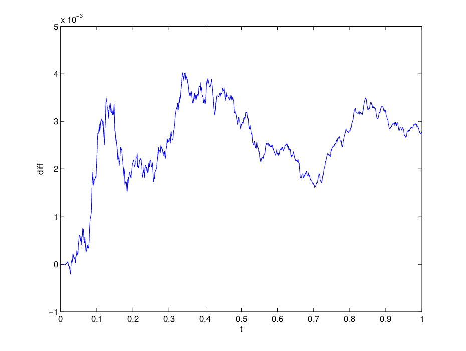
For α>0\alpha>0, no closed-form solution is available and we therefore use the Euler timestepping particle method from Kaushansky and Reisinger, (2018) with sufficiently many particles and timesteps as benchmark.

We illustrate the difference between our method and Kaushansky and Reisinger, (2018) in Figure 5.

Refer to caption
(a)
Refer to caption
(b)
Figure 5: Comparison of the numerical solution by Volterra equations (N=1000N=1000) with that of the particle method in Kaushansky and Reisinger, (2018) for α=0.5\alpha=0.5.

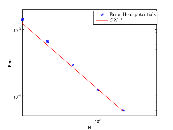
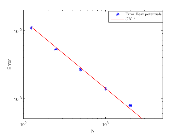
We now analyse the convergence order of the discretisation scheme for the Volterra equation empirically. With NN time steps, the error of the approximation (22) is expected to be O⁡(N−1)O(N^{-1}), because the trapezoidal integration in (16), (18), and (19) is on intervals (0,Δ)(0,\sqrt{\Delta}), and the result is divided by Δ\sqrt{\Delta} after that. We empirically confirm this in Figure 6.
Refer to caption
(a)
Refer to caption
(b)
Figure 6: Error in the maximum norm for numerical method in Section 4.2: (a) for gg compared to the exact solution for α=0\alpha=0; (b) for LL compared to the simulation solution for α=0.5\alpha=0.5.

The complexity of our method is O⁡(N2)O(N^{2}). Hence, in order to achieve precision ε\varepsilon, we need O⁡(ε−2)O(\varepsilon^{-2}) operations. In comparison, the particle method with Brownian bridge in Kaushansky and Reisinger, (2018) requires O⁡(ε−3)O(\varepsilon^{-3}) operations. The latter could be improved to O⁡(ε−2)O(\varepsilon^{-2}) by multilevel simulation, but equally a higher order method for the Volterra equation would bring the complexity down. Another advantage of the method above is that we automatically get directly the derivative gg of the loss function, which is harder to obtain in Kaushansky and Reisinger, (2018) because of Monte Carlo noise.

5.2 Comparison of perturbation and numerical methods

Here, we compare the numerical and perturbation solutions described above. We fix T=1T=1, z=0.5z=0.5, and choose N=1000N=1000, the number of grid points, sufficiently large so that the numerical error is negligible. In Figure 7 we plot gg, the hitting time density, computed with numerical and perturbation methods as well as g0​(t)g_{0}(t), the solution for α=0\alpha=0, to measure the impact of the nonlinear term, for different values of α\alpha. For α=0.1\alpha=0.1, the two solutions are visually indistinguishable; for α=0.3\alpha=0.3 there is small but visible difference between the solutions, which increases further for α=0.5\alpha=0.5 and arises from the higher order terms.22 2 In our implementation of the perturbation solution, we also perform a scaling to ensure the correct cumulative density at TT (which in practice is unknown) to improve the results slightly. For α=1\alpha=1, where the numerical solution shows a jump in the loss function at around t=0.1t=0.1, the first order expansion approximation breaks down.

Refer to caption
(a)
Refer to caption
(b)
Refer to caption
(c)
Refer to caption
(d)
Figure 7: Comparison of the numerical and perturbative methods for different values of α\alpha.: (a) α=0.1\alpha=0.1; (b) α=0.3\alpha=0.3; (c) α=0.5\alpha=0.5; (d) α=1\alpha=1. For visibility, we take N=100N=100 in the numerical method in the last plot.

5.3 Parameter studies

We now assess the impact of the mean-field interaction by varying the parameter α\alpha.

We fix T=1,z=0.5T=1,z=0.5, and choose N=1000N=1000, the number of the grid points. Figure 8 demonstrates the behavior of ν⁡(t)\nu(t) and g⁡(t)g(t) for different values of α\alpha, starting with α=0\alpha=0; for LtL_{t}, including a case with discontinuity, see already Figure 1.

Refer to caption
(a)
Refer to caption
(b)
Figure 8: (a) ν⁡(t)\nu(t) for different values of α\alpha. (b) g⁡(t)g(t) for different values of α\alpha.

To illustrate the impact of the interaction further, we consider the expectation and variance of the default time depending on α\alpha. Since the expectation is infinite, we restrict it to the interval (0,T)(0,T), i.e. consider 𝔼⁡[τ|τ<T]\mathbb{E}[\tau|\tau<T] and 𝕍⁡[τ|τ<T]\mathbb{V}[\tau|\tau<T]. These expectations must be finite for any fixed TT, and go to infinity when T→∞T\to\infty. The conditional density is then pτ|τ<T​(t)=pτ​(t)∫0Tpτ​(s)​𝑑sp_{\tau|\tau<T}(t)=\frac{p_{\tau}(t)}{\int_{0}^{T}p_{\tau}(s)\,ds} for t∈[0,T]t\in[0,T]. Using this, one can easily evaluate the moments numerically. We present the results in Figure 9. As expected, we observe that the expected default time and its variance become smaller with increasing of α\alpha, and grow with increasing TT.

Refer to caption
(a)
Refer to caption
(b)
Refer to caption
(c)
Refer to caption
(d)
Figure 9: (a) and (b): 𝔼⁡[τ|τ<T]\mathbb{E}[\tau|\tau<T]; (c) and (d) 𝕍⁡[τ|τ<T]\mathbb{V}[\tau|\tau<T] for different values of α\alpha and TT.

6 Conclusion

We have developed a semi-analytical approach to finding the density of interacting particles where their common downward drift increases in magnitude when particles hit a lower boundary, thus creating a positive feedback effect. This leads to a nonlinear and nonlocal parabolic equation. Using the method of heat potentials, we derived an equivalent coupled system of Volterra integral equations and solved it numerically, or by expansion for a small interaction parameter α\alpha. We confirmed empirically the convergence of order 11 of the numerical method and demonstrated its better complexity in comparison to the particle method in Kaushansky and Reisinger, (2018). There are striking financial implications as the computations uncover, in a very simplified setting, how mutual liabilities accelerate defaults of individual banks.

This paper raises several open questions. The numerical method for the system of Volterra equations can be improved using the methods we described at the beginning of Section 4.2; one can potentially analyse the convergence of the method for the blow-up case. Another interesting direction is to study a model with common noise as in Hambly and Sojmark, (2018) and Ledger and Sojmark, (2018) using the method of heat potentials. Lastly, it would be interesting to investigate an extension of the current paper for more complicated diffusion equations such as those in Nadtochiy and Shkolnikov, (2017) and Carrillo et al., (2013).

Acknowledgements: We thank Ben Hambly and Andreas Sojmark for discussions on the theoretical properties of their model and its link to the Stefan problem.

Appendix A Derivation of limits in Section 3

We start with (3.1). We split 𝕃1\mathbb{L}_{1} into two parts,

𝕃1=𝕃1(1)−𝕃1(2),\mathbb{L}_{1}=\mathbb{L}_{1}^{\left(1\right)}-\mathbb{L}_{1}^{\left(2\right)},

where

𝕃1(1)\displaystyle\mathbb{L}_{1}^{\left(1\right)} =limx→0​(x​∫0texp⁡(−(x−Ψ⁡(t,t′))22​(t−t′))2​π​(t−t′)3​ν​(t′)​d​t′),\displaystyle=\underset{x\rightarrow 0}{\lim}\left(x\int_{0}^{t}\frac{\exp\left(-\frac{\left(x-\Psi\left(t,t^{\prime}\right)\right)^{2}}{2\left(t-t^{\prime}\right)}\right)}{\sqrt{2\pi\left(t-t^{\prime}\right)^{3}}}\nu\left(t^{\prime}\right)dt^{\prime}\right),
𝕃1(2)\displaystyle\mathbb{L}_{1}^{\left(2\right)} =limx→0​∫0tΨ⁡(t,t′)​exp⁡(−(x−Ψ⁡(t,t′))22​(t−t′))2​π​(t−t′)3​ν​(t′)​d​t′.\displaystyle=\underset{x\rightarrow 0}{\lim}\int_{0}^{t}\frac{\Psi\left(t,t^{\prime}\right)\exp\left(-\frac{\left(x-\Psi\left(t,t^{\prime}\right)\right)^{2}}{2\left(t-t^{\prime}\right)}\right)}{\sqrt{2\pi\left(t-t^{\prime}\right)^{3}}}\nu\left(t^{\prime}\right)dt^{\prime}.

We represent ν⁡(t′)=ν⁡(t)+(ν⁡(t′)−ν⁡(t))\nu\left(t^{\prime}\right)=\nu\left(t\right)+\left(\nu\left(t^{\prime}\right)-\nu\left(t\right)\right), and write

𝕃1(1)\displaystyle\mathbb{L}_{1}^{\left(1\right)} =limx→0​(x​ν​(t)​∫0texp⁡(−(x−Ψ⁡(t,t′))22​(t−t′))2​π​(t−t′)3​d​t′)\displaystyle=\underset{x\rightarrow 0}{\lim}\left(x\nu\left(t\right)\int_{0}^{t}\frac{\exp\left(-\frac{\left(x-\Psi\left(t,t^{\prime}\right)\right)^{2}}{2\left(t-t^{\prime}\right)}\right)}{\sqrt{2\pi\left(t-t^{\prime}\right)^{3}}}\,dt^{\prime}\right)
+limx→0​(x​∫0texp⁡(−(x−Ψ⁡(t,t′))22​(t−t′))2​π​(t−t′)3​(ν⁡(t′)−ν⁡(t))​d​t′)\displaystyle+\underset{x\rightarrow 0}{\lim}\left(x\int_{0}^{t}\frac{\exp\left(-\frac{\left(x-\Psi\left(t,t^{\prime}\right)\right)^{2}}{2\left(t-t^{\prime}\right)}\right)}{\sqrt{2\pi\left(t-t^{\prime}\right)^{3}}}\left(\nu\left(t^{\prime}\right)-\nu\left(t\right)\right)\,dt^{\prime}\right)
=ν⁡(t)​limx→0​(x​∫0texp⁡(−(x−Ψ⁡(t,t′))22​(t−t′))2​π​(t−t′)3​d​t′),\displaystyle=\nu\left(t\right)\underset{x\rightarrow 0}{\lim}\left(x\int_{0}^{t}\frac{\exp\left(-\frac{\left(x-\Psi\left(t,t^{\prime}\right)\right)^{2}}{2\left(t-t^{\prime}\right)}\right)}{\sqrt{2\pi\left(t-t^{\prime}\right)^{3}}}\,dt^{\prime}\right),

since the second integral converges. We use the change of variables t−t′=x2​ut-t^{\prime}=x^{2}u, so that

limx→0​(x​∫0texp⁡(−(x−Ψ⁡(t,t′))22​(t−t′))2​π​(t−t′)3​d​t′)=limx→0​∫0t/x2exp⁡(−12​u)2​π​u3​du=∫0∞exp⁡(−12​u)2​π​u3​du=1.\displaystyle\underset{x\rightarrow 0}{\lim}\left(x\int_{0}^{t}\frac{\exp\left(-\frac{\left(x-\Psi\left(t,t^{\prime}\right)\right)^{2}}{2\left(t-t^{\prime}\right)}\right)}{\sqrt{2\pi\left(t-t^{\prime}\right)^{3}}}\,dt^{\prime}\right)=\underset{x\rightarrow 0}{\lim}\int_{0}^{t/x^{2}}\frac{\exp\left(-\frac{1}{2u}\right)}{\sqrt{2\pi u^{3}}}\,du=\int_{0}^{\infty}\frac{\exp\left(-\frac{1}{2u}\right)}{\sqrt{2\pi u^{3}}}\,du=1.

Since the second integral converges, it is clear that

𝕃1(2)=∫0tΨ⁡(t,t′)​Ξ​(t,t′)2​π​(t−t′)3​ν​(t′)​d​t′.\mathbb{L}_{1}^{\left(2\right)}=\int_{0}^{t}\frac{\Psi\left(t,t^{\prime}\right)\Xi\left(t,t^{\prime}\right)}{\sqrt{2\pi\left(t-t^{\prime}\right)^{3}}}\nu\left(t^{\prime}\right)dt^{\prime}.

Thus, (3.1) is valid.

The second limit 𝕃2\mathbb{L}_{2} in (3.2) is less standard and more difficult to evaluate. We introduce a non-singular function ϕ\phi,

ϕ⁡(t,t′)\displaystyle\phi\left(t,t^{\prime}\right) =Ψ⁡(t,t′)t−t′,t≠t′,ϕ(t,t)=Mt(t),\displaystyle=\frac{\Psi\left(t,t^{\prime}\right)}{t-t^{\prime}},\quad t\neq t^{\prime},\qquad\quad\phi\left(t,t\right)=M_{t}\left(t\right),

and write

𝕃2\displaystyle\mathbb{{L}}_{2} =limx→0​∫0t(1−x2(t−t′)+2​x​ϕ​(t,t′)−ϕ​(t,t′)2​(t−t′))\displaystyle=\underset{x\rightarrow 0}{\lim}\int_{0}^{t}\left(1-\frac{x^{2}}{\left(t-t^{\prime}\right)}+2x\phi\left(t,t^{\prime}\right)-\phi\left(t,t^{\prime}\right)^{2}\left(t-t^{\prime}\right)\right)
×exp⁡(−x22​(t−t′)+x​ϕ​(t,t′))​Ξ​(t,t′)2​π​(t−t′)3​ν​(t′)​d​t′\displaystyle\times\frac{\exp\left(-\frac{x^{2}}{2\left(t-t^{\prime}\right)}+x\phi\left(t,t^{\prime}\right)\right)\Xi\left(t,t^{\prime}\right)}{\sqrt{2\pi\left(t-t^{\prime}\right)^{3}}}\nu\left(t^{\prime}\right)\,dt^{\prime}
=𝕃2(1)+𝕃2(2)+2​𝕃2(3)−𝕃2(4),\displaystyle=\mathbb{{L}}_{2}^{\left(1\right)}+\mathbb{{L}}_{2}^{\left(2\right)}+2\mathbb{{L}}_{2}^{\left(3\right)}-\mathbb{{L}}_{2}^{\left(4\right)},

where

𝕃2(1)\displaystyle\mathbb{{L}}_{2}^{\left(1\right)} =limx→0​ν​(t)​∫0t(1−x2(t−t′))​exp⁡(−x22​(t−t′)+2​x​ϕ​(t,t′))2​π​(t−t′)3​d​t′,\displaystyle=\underset{x\rightarrow 0}{\lim}\,\nu\left(t\right)\int_{0}^{t}\left(1-\frac{x^{2}}{\left(t-t^{\prime}\right)}\right)\frac{\exp\left(-\frac{x^{2}}{2\left(t-t^{\prime}\right)}+2x\phi\left(t,t^{\prime}\right)\right)}{\sqrt{2\pi\left(t-t^{\prime}\right)^{3}}}\,dt^{\prime},
𝕃2(2)\displaystyle\mathbb{{L}}_{2}^{\left(2\right)} =limx→0​∫0t(1−x2(t−t′))​exp⁡(−x22​(t−t′)+2​x​ϕ​(t,t′))2​π​(t−t′)3​(Ξ⁡(t,t′)​ν​(t′)−ν⁡(t))​d​t′,\displaystyle=\underset{x\rightarrow 0}{\lim}\int_{0}^{t}\left(1-\frac{x^{2}}{\left(t-t^{\prime}\right)}\right)\frac{\exp\left(-\frac{x^{2}}{2\left(t-t^{\prime}\right)}+2x\phi\left(t,t^{\prime}\right)\right)}{\sqrt{2\pi\left(t-t^{\prime}\right)^{3}}}\left(\Xi\left(t,t^{\prime}\right)\nu\left(t^{\prime}\right)-\nu\left(t\right)\right)\,dt^{\prime},
𝕃2(3)\displaystyle\mathbb{{L}}_{2}^{\left(3\right)} =limx→0​x​∫0tϕ⁡(t,t′)​exp⁡(−x22​(t−t′)+2​x​ϕ​(t,t′))​Ξ​(t,t′)2​π​(t−t′)3​ν​(t′)​d​t′,\displaystyle=\underset{x\rightarrow 0}{\lim}\,x\int_{0}^{t}\phi\left(t,t^{\prime}\right)\frac{\exp\left(-\frac{x^{2}}{2\left(t-t^{\prime}\right)}+2x\phi\left(t,t^{\prime}\right)\right)\Xi\left(t,t^{\prime}\right)}{\sqrt{2\pi\left(t-t^{\prime}\right)^{3}}}\nu\left(t^{\prime}\right)\,dt^{\prime},
𝕃2(4)\displaystyle\mathbb{{L}}_{2}^{\left(4\right)} =limx→0​∫0tϕ​(t,t′)2​exp⁡(−x22​(t−t′)+x​ϕ​(t,t′))​Ξ​(t,t′)2​π​(t−t′)​ν​(t′)​d​t′.\displaystyle=\underset{x\rightarrow 0}{\lim}\int_{0}^{t}\phi\left(t,t^{\prime}\right)^{2}\frac{\exp\left(-\frac{x^{2}}{2\left(t-t^{\prime}\right)}+x\phi\left(t,t^{\prime}\right)\right)\Xi\left(t,t^{\prime}\right)}{\sqrt{2\pi\left(t-t^{\prime}\right)}}\nu\left(t^{\prime}\right)\,dt^{\prime}.

We have

𝕃2(1)\displaystyle\mathbb{{L}}_{2}^{\left(1\right)} =limx→0​ν​(t)​∫0t(1−x2(t−t′))​exp⁡(−x22​(t−t′)+2​x​ϕ​(t,t′))2​π​(t−t′)3​d​t′\displaystyle=\underset{x\rightarrow 0}{\lim}\,\nu\left(t\right)\int_{0}^{t}\left(1-\frac{x^{2}}{\left(t-t^{\prime}\right)}\right)\frac{\exp\left(-\frac{x^{2}}{2\left(t-t^{\prime}\right)}+2x\phi\left(t,t^{\prime}\right)\right)}{\sqrt{2\pi\left(t-t^{\prime}\right)^{3}}}\,dt^{\prime}
=ν⁡(t)​limx→0​1x​∫0t/x2(1−1u)​exp⁡(−12​u)2​π​u3​𝑑u\displaystyle=\nu\left(t\right)\underset{x\rightarrow 0}{\lim}\frac{1}{x}\int_{0}^{t/x^{2}}\left(1-\frac{1}{u}\right)\frac{\exp\left(-\frac{1}{2u}\right)}{\sqrt{2\pi u^{3}}}\,du
=2​ν​(t)​limx→0​1x​∫x/t∞(1−v2)​exp⁡(−v22)2​π​𝑑v\displaystyle=2\nu\left(t\right)\underset{x\rightarrow 0}{\lim}\frac{1}{x}\int_{x/\sqrt{t}}^{\infty}\left(1-v^{2}\right)\frac{\exp\left(-\frac{v^{2}}{2}\right)}{\sqrt{2\pi}}\,dv
=−2ν(t)limx→01x∫0x/t(1−v2)exp⁡(−v22)2​πdv\displaystyle=-2\nu\left(t\right)\underset{x\rightarrow 0}{\lim}\frac{1}{x}\int_{0}^{x/\sqrt{t}}\left(1-v^{2}\right)\frac{\exp\left(-\frac{v^{2}}{2}\right)}{\sqrt{2\pi}}\,dv
=−22​π​t​ν​(t),\displaystyle=-\frac{2}{\sqrt{2\pi t}}\nu\left(t\right),

where (t−t′)=u\left(t-t^{\prime}\right)=u, u=1/v2u=1/v^{2} and we have used the fact that

∫0∞(1−v2)​exp⁡(−v22)2​π​𝑑v=0.\int_{0}^{\infty}\left(1-v^{2}\right)\frac{\exp\left(-\frac{v^{2}}{2}\right)}{\sqrt{2\pi}}\,dv=0.

Further,

𝕃2(2)\displaystyle\mathbb{{L}}_{2}^{\left(2\right)} =limx→0​∫0t(1−x2(t−t′))​exp⁡(−x22​(t−t′)+2​x​ϕ​(t,t′))2​π​(t−t′)3​(Ξ⁡(t,t′)​ν​(t′)−ν⁡(t))​d​t′\displaystyle=\underset{x\rightarrow 0}{\lim}\int_{0}^{t}\left(1-\frac{x^{2}}{\left(t-t^{\prime}\right)}\right)\frac{\exp\left(-\frac{x^{2}}{2\left(t-t^{\prime}\right)}+2x\phi\left(t,t^{\prime}\right)\right)}{\sqrt{2\pi\left(t-t^{\prime}\right)^{3}}}\left(\Xi\left(t,t^{\prime}\right)\nu\left(t^{\prime}\right)-\nu\left(t\right)\right)\,dt^{\prime}
=limx→0​∫0texp⁡(−x22​(t−t′)+2​x​ϕ​(t,t′))2​π​(t−t′)3​(Ξ⁡(t,t′)​ν​(t′)−ν⁡(t))​d​t′\displaystyle=\underset{x\rightarrow 0}{\lim}\int_{0}^{t}\frac{\exp\left(-\frac{x^{2}}{2\left(t-t^{\prime}\right)}+2x\phi\left(t,t^{\prime}\right)\right)}{\sqrt{2\pi\left(t-t^{\prime}\right)^{3}}}\left(\Xi\left(t,t^{\prime}\right)\nu\left(t^{\prime}\right)-\nu\left(t\right)\right)\,dt^{\prime}
=∫0t(Ξ⁡(t,t′)​ν​(t′)−ν⁡(t))2​π​(t−t′)3​d​t′,\displaystyle=\int_{0}^{t}\frac{\left(\Xi\left(t,t^{\prime}\right)\nu\left(t^{\prime}\right)-\nu\left(t\right)\right)}{\sqrt{2\pi\left(t-t^{\prime}\right)^{3}}}\,dt^{\prime},

where we have dropped the higher order x2x^{2} term in the integral in the second line,

𝕃2(3)\displaystyle\mathbb{{L}}_{2}^{\left(3\right)} =limx→0​x​∫0tϕ⁡(t,t′)​exp⁡(−x22​(t−t′)+2​x​ϕ​(t,t′))2​π​(t−t′)3​Ξ​(t,t′)​ν​(t′)​d​t′\displaystyle=\underset{x\rightarrow 0}{\lim}x\int_{0}^{t}\phi\left(t,t^{\prime}\right)\frac{\exp\left(-\frac{x^{2}}{2\left(t-t^{\prime}\right)}+2x\phi\left(t,t^{\prime}\right)\right)}{\sqrt{2\pi\left(t-t^{\prime}\right)^{3}}}\Xi\left(t,t^{\prime}\right)\nu\left(t^{\prime}\right)\,dt^{\prime}
=ϕ⁡(t,t)​Ξ​(t,t)​ν​(t)=Mt​(t)​ν​(t),\displaystyle=\phi\left(t,t\right)\Xi\left(t,t\right)\nu\left(t\right)=M_{t}\left(t\right)\nu\left(t\right),

and

𝕃2(4)\displaystyle\mathbb{{L}}_{2}^{\left(4\right)} =limx→0​∫0tϕ​(t,t′)2​exp⁡(−x22​(t−t′)+x​ϕ​(t,t′))2​π​(t−t′)​Ξ​(t,t′)​ν​(t′)​d​t′\displaystyle=\underset{x\rightarrow 0}{\lim}\int_{0}^{t}\phi\left(t,t^{\prime}\right)^{2}\frac{\exp\left(-\frac{x^{2}}{2\left(t-t^{\prime}\right)}+x\phi\left(t,t^{\prime}\right)\right)}{\sqrt{2\pi\left(t-t^{\prime}\right)}}\Xi\left(t,t^{\prime}\right)\nu\left(t^{\prime}\right)\,dt^{\prime}
=∫0tϕ​(t,t′)2​Ξ⁡(t,t′)2​π​(t−t′)​ν​(t′)​d​t′=∫0tΨ​(t,t′)2(t−t′)​Ξ⁡(t,t′)2​π​(t−t′)3​ν​(t′)​d​t′.\displaystyle=\int_{0}^{t}\phi\left(t,t^{\prime}\right)^{2}\frac{\Xi\left(t,t^{\prime}\right)}{\sqrt{2\pi\left(t-t^{\prime}\right)}}\nu\left(t^{\prime}\right)\,dt^{\prime}=\int_{0}^{t}\frac{\Psi\left(t,t^{\prime}\right)^{2}}{\left(t-t^{\prime}\right)}\frac{\Xi\left(t,t^{\prime}\right)}{\sqrt{2\pi\left(t-t^{\prime}\right)^{3}}}\nu\left(t^{\prime}\right)\,dt^{\prime}.

Finally,

𝕃2\displaystyle\mathbb{{L}}_{2} =𝕃2(1)+𝕃2(2)+2​𝕃2(3)−𝕃2(4)\displaystyle=\mathbb{{L}}_{2}^{\left(1\right)}+\mathbb{{L}}_{2}^{\left(2\right)}+2\mathbb{{L}}_{2}^{\left(3\right)}-\mathbb{{L}}_{2}^{\left(4\right)}
=−2​12​π​t​ν​(t)+∫0t(Ξ⁡(t,t′)​ν​(t′)−ν⁡(t))2​π​(t−t′)3​d​t′\displaystyle=-2\frac{1}{\sqrt{2\pi t}}\nu\left(t\right)+\int_{0}^{t}\frac{\left(\Xi\left(t,t^{\prime}\right)\nu\left(t^{\prime}\right)-\nu\left(t\right)\right)}{\sqrt{2\pi\left(t-t^{\prime}\right)^{3}}}\,dt^{\prime}
+2​Mt​(t)​ν​(t)−∫0tΨ​(t,t′)2(t−t′)​Ξ⁡(t,t′)2​π​(t−t′)3​ν​(t′)​d​t′\displaystyle+2M_{t}\left(t\right)\nu\left(t\right)-\int_{0}^{t}\frac{\Psi\left(t,t^{\prime}\right)^{2}}{\left(t-t^{\prime}\right)}\frac{\Xi\left(t,t^{\prime}\right)}{\sqrt{2\pi\left(t-t^{\prime}\right)^{3}}}\nu\left(t^{\prime}\right)\,dt^{\prime}
=2​(Mt​(t)−12​π​t)​ν​(t)+∫0t((1−Ψ​(t,t′)2(t−t′))​Ξ​(t,t′)​ν​(t′)−ν⁡(t))2​π​(t−t′)3​d​t′,\displaystyle=2\left(M_{t}\left(t\right)-\frac{1}{\sqrt{2\pi t}}\right)\nu\left(t\right)+\int_{0}^{t}\frac{\left(\left(1-\frac{\Psi\left(t,t^{\prime}\right)^{2}}{\left(t-t^{\prime}\right)}\right)\Xi\left(t,t^{\prime}\right)\nu\left(t^{\prime}\right)-\nu\left(t\right)\right)}{\sqrt{2\pi\left(t-t^{\prime}\right)^{3}}}\,dt^{\prime},

as stated.

Appendix B Special cases

For illustration, we work out the solution from the formula obtained in Section 3 for two special cases which are also accessible by the standard reflection principle for Brownian motion or method of images for parabolic equations.

B.1 M⁡(t)=0M(t)=0

When M⁡(t)=0M\left(t\right)=0, we get

{ν⁡(t)+exp⁡(−z22​t)2​π​t=0,g⁡(t)+12​π​t​ν​(t)+12​∫0t(ν⁡(t)−ν⁡(t′))2​π​(t−t′)3​d​t′−z​exp⁡(−z22​t)2​2​π​t3=0.\left\{\begin{aligned} &\nu\left(t\right)+\frac{\exp\left(-\frac{z^{2}}{2t}\right)}{\sqrt{2\pi t}}=0,\\ &g\left(t\right)+\frac{1}{\sqrt{2\pi t}}\nu\left(t\right)+\frac{1}{2}\int_{0}^{t}\frac{\left(\nu\left(t\right)-\nu\left(t^{\prime}\right)\right)}{\sqrt{2\pi\left(t-t^{\prime}\right)^{3}}}\,dt^{\prime}-\frac{z\exp\left(-\frac{z^{2}}{2t}\right)}{2\sqrt{2\pi t^{3}}}=0.\end{aligned}\right.

Integration by parts of the second equation and use of the first yields

g⁡(t)\displaystyle g\left(t\right) =−∫0tν⋅​(t′)2​π​(t−t′)dt′+z​exp⁡(−z22​t)2​2​π​t3\displaystyle=-\int_{0}^{t}\frac{\overset{\cdot}{\nu}\left(t^{\prime}\right)}{\sqrt{2\pi\left(t-t^{\prime}\right)}}\,dt^{\prime}+\frac{z\exp\left(-\frac{z^{2}}{2t}\right)}{2\sqrt{2\pi t^{3}}}
=z​exp⁡(−z22​t)2​2​π​t3+z​exp⁡(−z22​t)2​2​π​t3\displaystyle=\frac{z\exp\left(-\frac{z^{2}}{2t}\right)}{2\sqrt{2\pi t^{3}}}+\frac{z\exp\left(-\frac{z^{2}}{2t}\right)}{2\sqrt{2\pi t^{3}}}
=z​exp⁡(−z22​t)2​π​t3,\displaystyle=\frac{z\exp\left(-\frac{z^{2}}{2t}\right)}{\sqrt{2\pi t^{3}}},

as expected.

B.2 M⁡(t)=μ​tM(t)=\mu t

When M⁡(t)=μ​tM\left(t\right)=\mu t, we get

{ν⁡(t)−μ​∫0texp⁡(−μ2​(t−t′)2)2​π​(t−t′)​ν​(t′)​d​t′+exp⁡(−(μ​t+z)22​t)2​π​t=0,g⁡(t)=12​2​π​∫0t1(t−t′)3​(exp⁡(−μ2​(t−t′)2)​ν​(t′)−ν⁡(t))​d​t′−μ22​2​π∫0t1t−t′exp(−μ2​(t−t′)2)ν(t′)dt′+(μ−12​π​t)ν(t)+(μ​t+z)​exp⁡(−(μ​t+z)22​t)2​π​t3.\left\{\begin{aligned} &\nu(t)-\mu\int_{0}^{t}\frac{\exp\left(-\frac{\mu^{2}(t-t^{\prime})}{2}\right)}{\sqrt{2\pi(t-t^{\prime})}}\nu(t^{\prime})dt^{\prime}+\frac{\exp\left(-\frac{(\mu t+z)^{2}}{2t}\right)}{\sqrt{2\pi t}}=0,\\ &g\left(t\right)=\frac{1}{2\sqrt{2\pi}}\int_{0}^{t}\frac{1}{\sqrt{(t-t^{\prime})^{3}}}\left(\exp\left(-\frac{\mu^{2}(t-t^{\prime})}{2}\right)\nu\left(t^{\prime}\right)-\nu(t)\right)dt^{\prime}\\ &-\frac{\mu^{2}}{2\sqrt{2\pi}}\int_{0}^{t}\frac{1}{\sqrt{t-t^{\prime}}}\exp\left(-\frac{\mu^{2}(t-t^{\prime})}{2}\right)\nu\left(t^{\prime}\right)dt^{\prime}+\left(\mu-\frac{1}{\sqrt{2\pi t}}\right)\nu(t)\\ &+\frac{\left(\mu t+z\right)\exp\left(-\frac{\left(\mu t+z\right)^{2}}{2t}\right)}{\sqrt{2\pi t^{3}}}.\end{aligned}\right. (23)

Taking the Laplace transform of the first equation in (23), we have

ν^​(s)−μ​ν^​(s)​12​s+μ2+exp⁡(−z​2​s+μ2−μ​z)2​s+μ2=0.\hat{\nu}(s)-\mu\hat{\nu}(s)\frac{1}{\sqrt{2s+\mu^{2}}}+\frac{\exp(-z\sqrt{2s+\mu^{2}}-\mu z)}{\sqrt{2s+\mu^{2}}}=0.

Hence,

ν^​(s)=−exp⁡(−z​2​s+μ2−μ​z)2​s+μ2−μ.\hat{\nu}(s)=-\frac{\exp(-z\sqrt{2s+\mu^{2}}-\mu z)}{\sqrt{2s+\mu^{2}}-\mu}.

The inverse Laplace transform of ν^​(s)\hat{\nu}(s) can be found analytically, but we do not need it to compute g⁡(t)g(t). Consider the second equation of (23). The first integral can be rewritten as

12​2​π​∫0t1(t−t′)3​(exp⁡(−μ2​(t−t′)2)​ν​(t′)−ν⁡(t))​d​t′\displaystyle\frac{1}{2\sqrt{2\pi}}\int_{0}^{t}\frac{1}{\sqrt{(t-t^{\prime})^{3}}}\left(\exp\left(-\frac{\mu^{2}(t-t^{\prime})}{2}\right)\nu\left(t^{\prime}\right)-\nu(t)\right)dt^{\prime}
=12​π​∫0t(exp⁡(−μ2​(t−t′)2)​ν​(t′)−ν⁡(t))​d​(1(t−t′))\displaystyle=\frac{1}{\sqrt{2\pi}}\int_{0}^{t}\left(\exp\left(-\frac{\mu^{2}(t-t^{\prime})}{2}\right)\nu\left(t^{\prime}\right)-\nu(t)\right)d\left(\frac{1}{\sqrt{(t-t^{\prime})}}\right)
=−12​π​t​(exp⁡(−μ2​t2)​ν​(0)−ν⁡(t))−12​π​∫0t1t−t′​exp⁡(−μ2​(t−t′)2)​ν˙​(t′)​d​t′\displaystyle=-\frac{1}{\sqrt{2\pi t}}\left(\exp\left(-\frac{\mu^{2}t}{2}\right)\nu\left(0\right)-\nu(t)\right)-\frac{1}{\sqrt{2\pi}}\int_{0}^{t}\frac{1}{\sqrt{t-t^{\prime}}}\exp\left(-\frac{\mu^{2}(t-t^{\prime})}{2}\right)\ \dot{\nu}\left(t^{\prime}\right)dt^{\prime}
−μ22​2​π∫0t1(t−t′)exp(−μ2​(t−t′)2)ν(t′)dt′.\displaystyle-\frac{\mu^{2}}{2\sqrt{2\pi}}\int_{0}^{t}\frac{1}{\sqrt{(t-t^{\prime})}}\exp\left(-\frac{\mu^{2}(t-t^{\prime})}{2}\right)\nu\left(t^{\prime}\right)dt^{\prime}.

Thus,

g⁡(t)\displaystyle g(t) =μ​ν​(t)−12​π​t​exp⁡(−μ2​t2)​ν​(0)−12​π​∫0t1t−t′​exp⁡(−μ2​(t−t′)2)​ν˙​(t′)​d​t′\displaystyle=\mu\nu(t)-\frac{1}{\sqrt{2\pi t}}\exp\left(-\frac{\mu^{2}t}{2}\right)\nu\left(0\right)-\frac{1}{\sqrt{2\pi}}\int_{0}^{t}\frac{1}{\sqrt{t-t^{\prime}}}\exp\left(-\frac{\mu^{2}(t-t^{\prime})}{2}\right)\ \dot{\nu}\left(t^{\prime}\right)dt^{\prime}
−μ22​π∫0t1(t−t′)exp(−μ2​(t−t′)2)ν(t′)dt′+(μ​t+z)​exp⁡(−(μ​t+z)22​t)2​2​π​t3.\displaystyle-\frac{\mu^{2}}{\sqrt{2\pi}}\int_{0}^{t}\frac{1}{\sqrt{(t-t^{\prime})}}\exp\left(-\frac{\mu^{2}(t-t^{\prime})}{2}\right)\nu\left(t^{\prime}\right)dt^{\prime}+\frac{\left(\mu t+z\right)\exp\left(-\frac{\left(\mu t+z\right)^{2}}{2t}\right)}{2\sqrt{2\pi t^{3}}}.

Taking Laplace transform of the last equation, we get

g^​(s)\displaystyle\hat{g}(s) =μ​ν^​(s)−12​s+μ2​ν​(0)−12​s+μ2​(s​ν^​(s)−ν⁡(0))−μ22​s+μ2​ν^​(s)\displaystyle=\mu\hat{\nu}(s)-\frac{1}{\sqrt{2s+\mu^{2}}}\nu(0)-\frac{1}{\sqrt{2s+\mu^{2}}}\left(s\hat{\nu}(s)-\nu(0)\right)-\frac{\mu^{2}}{\sqrt{2s+\mu^{2}}}\hat{\nu}(s)
+(12+μ2​2​s+μ2)​exp⁡(−z​2​s+μ2+μ​z)\displaystyle+\left(\frac{1}{2}+\frac{\mu}{2\sqrt{2s+\mu^{2}}}\right)\exp(-z\sqrt{2s+\mu^{2}}+\mu z)
=(−μ2​s+μ2−μ+s+μ22​s+μ2​12​s+μ2−μ2CLOSE\displaystyle=\left(-\frac{\mu}{\sqrt{2s+\mu^{2}}-\mu}+\frac{s+\mu^{2}}{\sqrt{2s+\mu^{2}}}\frac{1}{\sqrt{2s+\mu^{2}}-\mu^{2}}\right.
OPEN+12+μ2​2​s+μ2)​exp⁡(−z​2​s+μ2+μ​z)=exp⁡(−z​2​s+μ2+μ​z).\displaystyle\left.+\frac{1}{2}+\frac{\mu}{2\sqrt{2s+\mu^{2}}}\right)\exp(-z\sqrt{2s+\mu^{2}}+\mu z)=\exp(-z\sqrt{2s+\mu^{2}}+\mu z).

The inverse Laplace transform yields the final expression for g⁡(t)g(t)

g⁡(t)=z​exp⁡(−(z−μ​t)22​t)2​π​t3,g(t)=\frac{z\exp\left(-\frac{(z-\mu t)^{2}}{2t}\right)}{\sqrt{2\pi t^{3}}},

as expected.

Appendix C Proof of Lemma 1

Proof of Lemma 1. We start with the first term and judiciously use integration by parts several times to get

dd​t​∫0tΞ⁡(t,t′)​ν​(t′)2​π​(t−t′)​d​t′\displaystyle\frac{d}{dt}\int_{0}^{t}\frac{\Xi\left(t,t^{\prime}\right)\nu\left(t^{\prime}\right)}{\sqrt{2\pi\left(t-t^{\prime}\right)}}\,dt^{\prime}
=−2dd​t∫0tΞ(t,t′)ν(t′)d(t−t′)2​π\displaystyle=-2\frac{d}{dt}\int_{0}^{t}\Xi\left(t,t^{\prime}\right)\nu\left(t^{\prime}\right)d\sqrt{\frac{\left(t-t^{\prime}\right)}{2\pi}}
=2​dd​t​(Ξ⁡(t,0)​ν​(0)​t2​π+∫0t(t−t′)2​π​d​(Ξ⁡(t,t′)​ν​(t′)))\displaystyle=2\frac{d}{dt}\left(\Xi\left(t,0\right)\nu\left(0\right)\sqrt{\frac{t}{2\pi}}+\int_{0}^{t}\sqrt{\frac{\left(t-t^{\prime}\right)}{2\pi}}d\left(\Xi\left(t,t^{\prime}\right)\nu\left(t^{\prime}\right)\right)\right)
=(2​t​Ξt​(t,0)+Ξ⁡(t,0))​ν​(0)2​π​t+∫0t12​π​(t−t′)​d​(Ξ⁡(t,t′)​ν​(t′)−ν⁡(t))\displaystyle=\frac{\left(2t\Xi_{t}\left(t,0\right)+\Xi\left(t,0\right)\right)\nu\left(0\right)}{\sqrt{2\pi t}}+\int_{0}^{t}\frac{1}{\sqrt{2\pi\left(t-t^{\prime}\right)}}d\left(\Xi\left(t,t^{\prime}\right)\nu\left(t^{\prime}\right)-\nu\left(t\right)\right)
+2∫0t(t−t′)2​πd(Ξt(t,t′)ν(t′))\displaystyle+2\int_{0}^{t}\sqrt{\frac{\left(t-t^{\prime}\right)}{2\pi}}d\left(\Xi_{t}\left(t,t^{\prime}\right)\nu\left(t^{\prime}\right)\right)
=(2​t​Ξt​(t,0)+Ξ⁡(t,0))​ν​(0)2​π​t−Ξ⁡(t,0)​ν​(0)−ν⁡(t)2​π​t−12​∫0tΞ⁡(t,t′)​ν​(t′)−ν⁡(t)2​π​(t−t′)3​d​t′\displaystyle=\frac{\left(2t\Xi_{t}\left(t,0\right)+\Xi\left(t,0\right)\right)\nu\left(0\right)}{\sqrt{2\pi t}}-\frac{\Xi\left(t,0\right)\nu\left(0\right)-\nu\left(t\right)}{\sqrt{2\pi t}}-\frac{1}{2}\int_{0}^{t}\frac{\Xi\left(t,t^{\prime}\right)\nu\left(t^{\prime}\right)-\nu\left(t\right)}{\sqrt{2\pi\left(t-t^{\prime}\right)^{3}}}\,dt^{\prime}
−2​Ξt​(t,0)​ν​(0)​t2​π+∫0tΞt​(t,t′)2​π​(t−t′)​ν​(t′)​d​t′\displaystyle-2\Xi_{t}\left(t,0\right)\nu\left(0\right)\sqrt{\frac{t}{2\pi}}+\int_{0}^{t}\frac{\Xi_{t}\left(t,t^{\prime}\right)}{\sqrt{2\pi\left(t-t^{\prime}\right)}}\nu\left(t^{\prime}\right)\,dt^{\prime}
=ν⁡(t)2​π​t+12​∫0tν⁡(t)−(Ξ⁡(t,t′)−2​(t−t′)​Ξt​(t,t′))​ν​(t′)2​π​(t−t′)3​d​t′\displaystyle=\frac{\nu\left(t\right)}{\sqrt{2\pi t}}+\frac{1}{2}\int_{0}^{t}\frac{\nu\left(t\right)-\left(\Xi\left(t,t^{\prime}\right)-2\left(t-t^{\prime}\right)\Xi_{t}\left(t,t^{\prime}\right)\right)\nu\left(t^{\prime}\right)}{\sqrt{2\pi\left(t-t^{\prime}\right)^{3}}}\,dt^{\prime}
=ν⁡(t)2​π​t+∫0t(ν⁡(t)−(Ξ⁡(t,t′)−2​(t−t′)​Ξt​(t,t′))​ν​(t′))​d​(12​π​(t−t′))\displaystyle=\frac{\nu\left(t\right)}{\sqrt{2\pi t}}+\int_{0}^{t}\left(\nu\left(t\right)-\left(\Xi\left(t,t^{\prime}\right)-2\left(t-t^{\prime}\right)\Xi_{t}\left(t,t^{\prime}\right)\right)\nu\left(t^{\prime}\right)\right)d\left(\frac{1}{\sqrt{2\pi\left(t-t^{\prime}\right)}}\right)
=∫0t((Ξ⁡(t,t′)−2​(t−t′)​Ξt​(t,t′))​ν​(t′))t′2​π​(t−t′)​d​t′.\displaystyle=\int_{0}^{t}\frac{\left(\left(\Xi\left(t,t^{\prime}\right)-2\left(t-t^{\prime}\right)\Xi_{t}\left(t,t^{\prime}\right)\right)\nu\left(t^{\prime}\right)\right)_{t^{\prime}}}{\sqrt{2\pi\left(t-t^{\prime}\right)}}\,dt^{\prime}.


References

  • Antonelli et al., (2002) Antonelli, F., Kohatsu-Higa, A., et al. (2002). Rate of convergence of a particle method to the solution of the McKean–Vlasov equation. The Annals of Applied Probability, 12(2):423–476.
  • Borkar and Suresh Kumar, (2010) Borkar, V. and Suresh Kumar, K. (2010). McKean–Vlasov limit in portfolio optimization. Stochastic Analysis and Applications, 28(5):884–906.
  • Bossy and Talay, (1997) Bossy, M. and Talay, D. (1997). A stochastic particle method for the McKean-Vlasov and the Burgers equation. Mathematics of Computation, 66(217):157–192.
  • Brunner, (1985) Brunner, H. (1985). The numerical solution of weakly singular Volterra integral equations by collocation on graded meshes. Mathematics of Computation, 45(172):417–437.
  • Bujok and Reisinger, (2012) Bujok, K. and Reisinger, C. (2012). Numerical valuation of basket credit derivatives in structural jump-diffusion models. Journal of Computational Finance, 15(4):115.
  • Bush et al., (2011) Bush, N., Hambly, B. M., Haworth, H., Jin, L., and Reisinger, C. (2011). Stochastic evolution equations in portfolio credit modelling. SIAM Journal on Financial Mathematics, 2(1):627–664.
  • Cáceres et al., (2011) Cáceres, M. J., Carrillo, J. A., and Perthame, B. (2011). Analysis of nonlinear noisy integrate & fire neuron models: blow-up and steady states. The Journal of Mathematical Neuroscience, 1(1):7.
  • Carrillo et al., (2013) Carrillo, J. A., González, M. d. M., Gualdani, M. P., and Schonbek, M. E. (2013). Classical solutions for a nonlinear Fokker–Planck equation arising in computational neuroscience. Communications in Partial Differential Equations, 38(3):385–409.
  • David and Lehar, (2014) David, A. and Lehar, A. (2014). Why are banks highly interconnected? Available at SSRN 1108870.
  • (10) Delarue, F., Inglis, J., Rubenthaler, S., and Tanré, E. (2015a). Global solvability of a networked integrate-and-fire model of McKean–Vlasov type. The Annals of Applied Probability, 25(4):2096–2133.
  • (11) Delarue, F., Inglis, J., Rubenthaler, S., and Tanré, E. (2015b). Particle systems with a singular mean-field self-excitation. Application to neuronal networks. Stochastic Processes and their Applications, 125(6):2451–2492.
  • Eisenberg and Noe, (2001) Eisenberg, L. and Noe, T. H. (2001). Systemic risk in financial systems. Management Science, 47(2):236–249.
  • Gobet and Pagliarani, (2018) Gobet, E. and Pagliarani, S. (2018). Analytical approximations of non-linear SDEs of McKean–Vlasov type. Journal of Mathematical Analysis and Applications, 466(1):71–106.
  • Hairer et al., (1985) Hairer, E., Lubich, C., and Schlichte, M. (1985). Fast numerical solution of nonlinear Volterra convolution equations. SIAM Journal on Scientific and Statistical Computing, 6(3):532–541.
  • Haji-Ali and Tempone, (2018) Haji-Ali, A.-L. and Tempone, R. (2018). Multilevel and Multi-index Monte Carlo methods for the McKean–Vlasov equation. Statistics and Computing, 28(4):923–935.
  • Hambly et al., (2018) Hambly, B., Ledger, S., and Sojmark, A. (2018). A McKean–Vlasov equation with positive feedback and blow-ups. arXiv preprint arXiv:1801.07703.
  • Hambly and Sojmark, (2018) Hambly, B. and Sojmark, A. (2018). An SPDE model for systemic risk with endogenous contagion. arXiv preprint arXiv:1801.10088.
  • Huang et al., (2006) Huang, M., Malhamé, R. P., Caines, P. E., et al. (2006). Large population stochastic dynamic games: closed-loop McKean–Vlasov systems and the Nash certainty equivalence principle. Communications in Information & Systems, 6(3):221–252.
  • Ichiba et al., (2018) Ichiba, T., Ludkovski, M., and Sarantsev, A. (2018). Dynamic contagion in a banking system with births and defaults. arXiv preprint arXiv:1807.09897.
  • Itkin and Lipton, (2015) Itkin, A. and Lipton, A. (2015). Efficient solution of structural default models with correlated jumps and mutual obligations. International Journal of Computer Mathematics, 92(12):2380–2405.
  • Itkin and Lipton, (2017) Itkin, A. and Lipton, A. (2017). Structural default model with mutual obligations. Review of Derivatives Research, 20:15–46.
  • Kac, (1956) Kac, M. (1956). Foundations of kinetic theory. In Proceedings of the Third Berkeley Symposium on Mathematical Statistics and Probability, volume 3, pages 171–197. University of California Press Berkeley and Los Angeles, California.
  • (23) Kaushansky, V., Lipton, A., and Reisinger, C. (2018a). Numerical analysis of an extended structural default model with mutual liabilities and jump risk. Journal of Computational Science, 24:218–231.
  • (24) Kaushansky, V., Lipton, A., and Reisinger, C. (2018b). Transition probability of Brownian motion in the octant and its application to default modelling. Applied Mathematical Finance. https://doi.org/10.1080/1350486X.2018.1481439.
  • Kaushansky and Reisinger, (2018) Kaushansky, V. and Reisinger, C. (2018). Simulation of particle systems interacting through hitting times. arXiv preprint arXiv:1805.11678.
  • Kolk and Pedas, (2009) Kolk, M. and Pedas, A. (2009). Numerical solution of Volterra integral equations with weakly singular kernels which may have a boundary singularity. Mathematical Modelling and Analysis, 14(1):79–89.
  • Kolk and Pedas, (2013) Kolk, M. and Pedas, A. (2013). Numerical solution of Volterra integral equations with singularities. Frontiers of Mathematics in China, 8(2):239–259.
  • Kolk et al., (2009) Kolk, M., Pedas, A., and Vainikko, G. (2009). High-order methods for Volterra integral equations with general weak singularities. Numerical Functional Analysis and Optimization, 30(9-10):1002–1024.
  • Ledger and Sojmark, (2018) Ledger, S. and Sojmark, A. (2018). At the mercy of the common noise: blow-ups in a conditional McKean–Vlasov problem. arXiv preprint arXiv:1807.05126.
  • Linz, (1985) Linz, P. (1985). Analytical and Numerical Methods for Volterra Equations. SIAM.
  • Lipton, (2001) Lipton, A. (2001). Mathematical Methods For Foreign Exchange: A Financial Engineer’s Approach. World Scientific.
  • Lipton, (2016) Lipton, A. (2016). Modern monetary circuit theory, stability of interconnected banking network, and balance sheet optimization for individual banks. International Journal of Theoretical and Applied Finance, 19(6). doi: 10.1142/S0219024916500345.
  • Lipton and Sepp, (2009) Lipton, A. and Sepp, A. (2009). Credit value adjustment for credit default swaps via the structural default model. The Journal of Credit Risk, 5(2):123–146.
  • Maleknejad et al., (2011) Maleknejad, K., Hashemizadeh, E., and Ezzati, R. (2011). A new approach to the numerical solution of Volterra integral equations by using Bernstein’s approximation. Communications in Nonlinear Science and Numerical Simulation, 16(2):647–655.
  • Maleknejad et al., (2007) Maleknejad, K., Sohrabi, S., and Rostami, Y. (2007). Numerical solution of nonlinear Volterra integral equations of the second kind by using Chebyshev polynomials. Applied Mathematics and Computation, 188(1):123–128.
  • McKean, (1966) McKean, H. P. (1966). A class of Markov processes associated with nonlinear parabolic equations. Proceedings of the National Academy of Sciences, 56(6):1907–1911.
  • Merton, (1974) Merton, R. C. (1974). On the pricing of corporate debt: The risk structure of interest rates. The Journal of Finance, 29(2):449–470.
  • Nadtochiy and Shkolnikov, (2017) Nadtochiy, S. and Shkolnikov, M. (2017). Particle systems with singular interaction through hitting times: application in systemic risk modeling. arXiv preprint arXiv:1705.00691.
  • Nadtochiy and Shkolnikov, (2018) Nadtochiy, S. and Shkolnikov, M. (2018). Mean field systems on networks, with singular interaction through hitting times. arXiv preprint arXiv:1807.02015.
  • Noble, (1969) Noble, B. (1969). Instability when solving Volterra integral equations of the second kind by multistep methods. In Conference on the numerical solution of differential equations, pages 23–39. Springer.
  • Peskir, (2002) Peskir, G. (2002). On integral equations arising in the first-passage problem for Brownian motion. The Journal of Integral Equations and Applications, pages 397–423.
  • Reis et al., (2018) Reis, G. d., Smith, G., and Tankov, P. (2018). Importance sampling for McKean-Vlasov SDEs. arXiv preprint arXiv:1803.09320.
  • Ricketson, (2015) Ricketson, L. (2015). A multilevel Monte Carlo method for a class of McKean–Vlasov processes. arXiv preprint arXiv:1508.02299.
  • Rubinstein, (1971) Rubinstein, L. (1971). The Stefan Problem, volume 27 of Translations of Mathematical Monographs. American Mathematical Society, Providence, RI.
  • Szpruch et al., (2017) Szpruch, L., Tan, S., and Tse, A. (2017). Iterative particle approximation for McKean–Vlasov SDEs with application to Multilevel Monte Carlo estimation. arXiv preprint arXiv:1706.00907.
  • Tikhonov and Samarskii, (1963) Tikhonov, A. N. and Samarskii, A. A. (1963). Equations of Mathematical Physics. Dover Publications, New York. English translation.
  • Watson, (2012) Watson, N. A. (2012). Introduction to Heat Potential Theory. Number 182 in Mathematical Surveys and Monographs. American Mathematical Soc.