Neuromorphic computing in Ginzburg-Landau polariton lattice systems
Abstract
The availability of large amounts of data and the necessity to process it efficiently have led to rapid development of machine learning techniques. To name a few examples, artificial neural network architectures are commonly used for financial forecasting, speech and image recognition, robotics, medicine, and even research. Direct hardware for neural networks is highly sought for overcoming the von Neumann bottleneck of software implementations. Reservoir computing (RC) is a recent and increasingly popular bio-inspired computing scheme which holds promise for an efficient temporal information processing. We demonstrate the applicability and performance of reservoir computing in a general complex Ginzburg-Landau lattice model, which adequately describes dynamics of a wide class of systems, including coherent photonic devices. In particular, we propose that the concept can be readily applied in exciton-polariton lattices, which are characterized by unprecedented photonic nonlinearity, opening the way to signal processing at rates of the order of 1 Tbit s-1.
I Introduction
In contrast to single- or multilayer (deep) feedforward networks, recurrent neural networks (RNNs) may exhibit complex internal state dynamics. This makes them particularly efficient in the analysis of time-dependent signals that require memory, such as speech or text recognition and interpretation [1]. On the other hand, training of RNNs is difficult and not always convergent. The idea of reservoir computing (RC), also known as echo state networks or liquid state machines, may be viewed as a generalization of the RNN concept, inspired by the internal structure of the brain [2, 3, 4, 5].
The core of the system is formed by a recurrent network of nodes (neurons) connected with each other, see Fig. 1. This network, called the reservoir, is static as its connections are unchanged during training. This is important for both the feasibility of a physical implementation and the convergence of the training procedure. Typically, the input signal represented by is multiplied by random weights and injected into reservoir nodes. The subsequent dynamics of amplitudes in the nodes (called neuron activations) is delivered to output neurons that are used e.g. for classification or prediction of time-dependent signals. In the classification task, the output neuron with the highest activation is identified with the predicted class. A supervised training procedure consists of presenting many different inputs to the system, and adjusting the output weights to minimize the average error. Output signals are linear superpositions of the amplitudes of the reservoir, which results in a training procedure that is both efficient and convergent [6].

The simple scheme described above proved to be surprisingly efficient in various machine learning tasks. The performance of RC in time series prediction and speech recognition is particularly well described [2, 7, 8, 9, 10, 11, 12]. Notably, software implementation of RC won a financial time series prediction competition [13]. To date, RC has been successfully realized not only as a software, but also as hardware implementations in systems including semiconductor chips [14], memristor arrays [15, 16] optoelectronic [17, 18, 7] and all-optical systems [19], mechanical oscillators [20] and even in a bucket of water [21]. See [22] for a comprehensive review. Photonic systems are particularly interesting as they hold promise for huge signal processing rates [11, 8, 7, 23, 24].
In many machine learning approaches, input data is transformed in a multidimensional space according to a nonlinear map. This nonlinear mapping in RC is typically provided by the complex dynamics of the reservoir, although nonlinear readout has also been implemented [11]. To be useful for computing, the network has to posses several characteristics. First, the size of the reservoir must be sufficiently large, so that it is able to perform the desired computation within its fixed internal structure. The so-called echo state property [5] is related to the stability of the system. The state of the reservoir must be determined solely by the history of the signal , but for sufficiently long evolution it should not depend on the initial conditions or signals from the distant past. On the other hand, the dynamics must be sufficiently nonlinear, so that the state of the reservoir allows for the separation of signals that differ by a small amount. The optimal working point appears to be placed close to a certain stability threshold [11, 6]. Importantly, it has been demonstrated that powerful computation can be achieved in a variety of different designs and systems. For instance, according to the original idea, reservoir nodes are connected with each other with random weights [2]. However, various other designs proved to be efficient as well [12, 11, 7].
In this work, we consider the implementation of RC in systems described by the complex Ginzburg-Landau equation (CGLE), which is one of the fundamental models of wave phenomena [25]. It provides a universal description of weakly nonlinear spatiotemporal systems invariant under a global gauge change , where typically is a slowly varying envelope of an oscillatory wave packet. Its range of applications spans from the description of hydrodynamic systems and chemical reactions, to superconductors and superfluids, to ultracold quantum gases and lasers [25, 26, 27]. We propose to implement reservoir dynamics in a lattice of weakly coupled traps with nearest neighbor couplings. According to our estimates, semiconductor exciton-polariton microcavity systems appear to be a promising platform for reservoir computing with very high signal processing data rates, which can be achieved thanks to the extremely strong optical nonlinearity on a picosecond timescale [28].
II Model
We consider the discrete version of the CGLE, which describes a system enclosed in a simple two-dimensional array of weakly coupled traps
| (1) |
where the first term on the right hand side corresponds to coherent signal injection with being the mask applied to the signal , see Fig. 2. Coupling coefficients between nearest-neighbor lattice sites are denoted by , is the gain coefficient, in general equal to the difference between the pumping rate () and the linear decay rate (), is the nonlinear decay rate, and is the conservative nonlinear coefficient.

The geometry of the lattice and the scheme of the experiment designed for a classification task is shown in Fig. 2. In our numerical simulations, we consider a simple rectangular lattice reservoir with random positive symmetric nearest-neighbor couplings, which is a natural choice for photonic systems such as microcavities, photonic crystals or waveguide arrays. Note that simpler geometries, such as a one-dimensional lattice with identical couplings and even single site systems have been demonstrated to perform well in experimental tests [9, 17, 7, 12]. The two-dimensional multisite system has, however, advantage in terms of increased efficiency.
The parameters of the model (1) used in numerical simulations are chosen to correspond to a lattice of coupled semiconductor exciton-polariton microcavities [29, 30, 31, 32]. Exciton-polaritons are composite quantum quasiparticles of semiconductor excitations and photons in the strong coupling regime [33, 34, 35]. They exhibit an interesting combination of properties of matter and light. The extremely low effective mass of polaritons, of the order of electron mass, results from the photonic component, and allows for the effective transport across the lattice on a picosecond timescale. On the other hand, the interaction resulting from the exciton component provides unprecedented instantaneous nonlinearity , orders of magnitude stronger than in other photonic systems [28]. These properties have been used recently to demonstrate remarkable phenomena including nonequilibrium condensation and lasing and superfluidity of polaritons [36, 37, 38, 39] as well as realization of ultrafast all-optical switches [40, 41, 42]. Recently, a single layer neural network design was proposed [43]. Note that reservoir computing should not be confused with the exciton reservoir, which consists of incoherent particles in the lasing regime. Here, we neglect the influence of exciton reservoir on the dynamics of the system, which can be achieved by an appropriate pumping scheme [44]. Our results apply to a range of other systems thanks to the universality of the CGLE equation and its scaling properties, which allow to convey them to other systems with different values of physical parameters in the CGLE equation (1) (details of the rescaling are given in the Appendix A).
III Results
We present results for handwritten digit recognition using the modified National Institute of Standards and Technology (MNIST) dataset, which is one of the standard tests of pattern recognition in machine learning. Additional simulations for the Mackey-Glass nonlinear system prediction task and speech recognition are presented in the Appendix D and E. The goal of the MNIST recognition task is to classify the digits of various writers using the recorded grayscale images. The dataset contains 70,000 digits, and in our simulations for training (4,000 digits) and testing (1,000 digits) we used randomly picked subsets of the whole set. Each digit consists of 2020 grayscale pixels.
We convert each image of a digit into temporal signals according to the scheme illustrated in Fig. 2, with pixels in each row converted into step-wise signals , where is the row number. The temporal length corresponding to a single pixel is adjusted to achieve optimal recognition rate. This parameter must be adjusted so that the timescales of the reservior and of the input signal are compatible, but the overall performance is not very sensitive to its value. The signal vector is multiplied by a random, constant matrix of dimension , which has the purpose of both distributing the information across the lattice and adjusting the length of the input vector to the number of pillars in the lattice . The incoming signal initiates dynamics of complex reservoir amplitudes , which correspond to neuron activations. The squared modulus of each lattice site is recorded at the end of the sequence. A linear transformation is used to translate the readout into output neuron activations, , where and is the length of the sequence. In the training phase, logistic regression is used to obtain optimal output weights (see Appendix C). During testing, the obtained are used to classify the digit. Ideally, the result is equal to for the correct digit and for all other digits. In practice, all have mixed values, and we choose the one that is the highest as the predicted digit.

An example of the resulting error rates is presented in Fig. 3. The average accuracy for this particular lattice is , higher than the one obtained by a linear classifier [45]. Additionally, we note that due to the reduced dimensionality of the output () with respect to the input (), the regression performed during the learning phase requires much less computation time. This is important if the minimization of error, performed offline, turns out to be the most time consuming part of teaching. At the same time, no offline computations are required during testing, and the recognition rate is limited only by the reservoir dynamics timescale.
We used realistic parameters that correspond to experiments performed in gallium arsenide polariton lattices [31, 32], with couplings distributed randomly between zero and meV, eV, and eV, ps. Signal processing on a picosecond timescale can be achieved thanks to the use of a photonic system with a very strong nonlinearity in the regime of quantum coupling of light and matter. According to our simulation, the typical rate at which data can be fed into each lattice site and processed efficiently is one byte (understood as a unit of information) every few tens of picoseconds. This estimation is in agreement with numerous time-resolved experiments in polariton systems performed in the nonlinear regime [46, 47, 48, 49, 50]. In contrast to single site RC systems, here signal processing is performed at nodes in a truly parallel manner. A lattice of a hundred of nodes should enable a realistic data rate of the order of 1 Tbit s-1, in a micrometer sized system. This compares favorably even with state of the art optoelectronic [8] and passive photonic microcircuit [11] RC implementations, which recently achieved 10 Gbit s-1 data rates.

Figure 4 shows the dependence of the error rate on the effective gain parameter . RC systems display optimal performance when in the absence of input signal the system is stable, but close to an instability threshold. In the case of CGLE, at the zero gain point the trivial solution () loses stability and a new stationary state appears. This threshold is interpreted in the exciton-polariton context as the onset of polariton lasing. It is clear from Fig. 4 that an optimal working point is found close to zero gain, or at the lasing threshold.

We present the dependence of the error rate on the size of the lattice in Fig. 5. In this Figure, error rates are calculated as a result of averaging over 10 different simulations corresponding to different random weights in the reservoir and in the input matrix . Since the input data is convoluted with random weights before being used for excitation, adjusting the number of rows in the rectangular matrix allows for imprinting the data on an arbitrary sized lattice. While in the case redundancy in the input is unavoidable, the same signal may be processed in various ways in different parts of the reservoir, which leads to improvement of the overall performance. Indeed, as shown in Fig. 5, the error rate consistently decreases with , and the error rate for a lattice is as low as , similar to a feedforward neural network with a single hidden layer [45]. The recognition rate in the case of a lattice is equal to , similar as in a memristor array RC of comparable size [15], but the readout vector size is much smaller in our case (100 variables versus a network).
As the error rate decreases with the system size, one can expect that the larger Hilbert space of quantum systems could offer increased performance [10] compared to their classical counterparts. Indeed, in the Appendix F, we find a reduced error rate if one has access to additional non-classical observables. However, given the additional complexity of measuring these quantities, the quantum advantage would not necessarily be more practical.
IV Discussion
In this work, we demonstrate the applicability of the reservoir computing framework in the wide class of systems described by the CGLE. We would like to point out that the majority of previously considered systems, including optoelectronic ones, were based on amplitude-dependent nonlinearity. On the other hand, the investigated CGLE model describes evolution of a complex wavefunction, where the couplings between nodes are represented by imaginary values, as in the second term in Eq. (1), and the nonlinearity relies on phase modulation (the g interaction constant), which is very different from the amplitude nonlinearity. Our results extend the applicability of reservoir computing to an important class of weakly nonlinear wave systems with gauge invariance, which include coherent photonic systems. Importantly, our scheme is robust to both disorder and dissipation, which are usually hindrances in information processing schemes. Here, dissipation is useful for ensuring the echo state property, and a disordered network of connections is part of the design. We also demonstrate robustness of the model against spatiotemporal noise (see Appendix B).
To illustrate the theoretical performance of the proposed system, we estimate the data processing rate and compare it with hardware implementations of reservoir neural networks realized experimentally. As the MNIST digit recognition task has not been implemented in many works on RC, we use the TI 46 speech recognition task as a benchmark. The details of the implementation in the case of an exciton-polariton network are given in Appendix E. Our numerical simulations demonstrate the estimated processing rate of words/s, compared to words/s reported in a CMOS FPGA implementation of liquid state machines [51], and the record high processing rate of words/s achieved in an optoelectronic delay line system [7]. The very high estimated processing rate of exciton-polariton systems results from the strong optical nonlinearity on a picosecond timescale and the parallel processing in each node of the lattice.
In terms of scalability of the system size, we note that polariton lattices with several thousands of pillar nodes have already been fabricated and investigated experimentally [52]. One can also estimate the physical size scalability with respect to other (non-RC) neuromorphic implementations. For example, the IBM TrueNorth chip [53] contains one million neurons on an approximate surface of 2 cm2, which gives an average of 5 000 neurons/mm2. A typical size of a polariton pillar node is m2, which gives an estimate of 100 000 nodes/mm2. While nodes in the RC framework are not equivalent to neurons in other architectures, which usually have some tunability, this estimate indicates that at least in some applications polariton RC could be competitive with respect to state-of-the-art neuromorphic systems.
From the point of view of energy efficiency, an important advantage of exciton-polariton systems is that they belong to the class of photonic (neutral particle) systems, which do not suffer from radiative heating, an important issue limiting further development of CMOS and other electronic technologies. Since excitons are neutral particles, they also do not contribute to radiative heating. Energy loss in polariton lattices results mostly from the escape of photons through imperfect microcavity mirrors. However, this does not impose a fundamental limit on energy efficiency (contrary to radiative heating in electronic systems), and several solutions can be proposed to suppress this loss channel. For example, transverse photon modes trapped by total internal reflection can be used to reduce polariton decay through the mirrors [28].
Acknowledgements.
AO acknowledges support from the National Science Center, Poland grant No. 2016/22/E/ST3/00045. MM acknowledges support from the National Science Center, Poland grant No. 2017/25/Z/ST3/03032 under QuantERA programme. SG and TL acknowledge support from the Singapore Ministry of Education (via the AcRF Tier 2 grant MOE2017-T2-1-001).Appendix A Scaling properties of the complex Ginzburg-Landau equation
The discrete complex Ginzburg–Landau equation with noise reads
| (2) |
The simplicity of Eq. (2) allows for the rescaling of physical coefficients using two arbitrary scaling parameters and , according to , , , , , , , . The dynamics of the system with tildes will be identical to the original one except for the difference in the timescale and amplitude of the wavefunction. It follows that the only relevant parameters that govern the qualitative behavior of the system are the ratio , and the relative values of coefficients , , and . In numerical simulations, the random values in the nearest-neighbor weight matrix and in matrix are created by the uniform pseudorandom number generator. The function is representing the Langevin noise with being the noise strength.
Appendix B The effect of noise
The additional Langevin noise term is representing noise in the system which is random in space and time. The effect of noise on the prediction error for the MNIST and speech recognition tasks is presented in Figs. 6 and 8, respectively.

Appendix C Logistic regression
We use a logistic regression algorithm to train the readout function for the digit recognition task. The values between 0 and 1 are assigned by a linear regression classifier to the output values for each vector containing elements.
We introduce the hypothesis function given by
| (3) |
where is the weights vector. For classification of the hypothesis representation we introduce the function
| (4) |
where is given by the logistic function
| (5) |
Combining the above equations the hypothesis function reads
| (6) |
The cost function is described by the equation
| (7) | ||||
where is the number of samples and is the correct output for given input states . We minimize the cost function by the gradient method
| (8) |
Weights are calculated using Matlab 2016 software with function "fmincg()" written by Carl Edward Rasmussen.
Appendix D The Mackey-Glass prediction task

Using the reservoir, we want to predict the solution of the Mackey-Glass equation:
| (9) |
which is a nonlinear differential equation with time delay feedback. We use the parameters , , , . Using a set of training data we would like to find output weights such that
| (10) |
where the feedback , where is a small time step. As a performance measure, we use the normalized mean square error (NRSE):
| (11) |
where and are the true solution of the Mackey-Glass equation and the corresponding prediction from the reservoir computer at time , respectively.
Appendix E Speech recognition
Here we consider the task of isolated spoken digit recognition, which has been a commonly considered benchmarking task for reservoir computing systems [17, 18, 11]. We use a standard data set, which was collected at Texas Instruments (TI) in 1980 (The NIST TI 46 corpus, which is available from the Linguistic Data Consortium). The data is a set of ten isolated spoken digits ( to ) by different female individuals. In the training set, each individual uttered times a digit, resulting total spoken digits. After training the network, we evaluate the success rate of our system by using an additional spoken digits ( digits spoken times by the individuals).

Each recorded piece of speech is sampled at 12.5 kHz, which is then converted into a cochleagram using the Lyon cochlear ear model [55], previously identified as a good form of preprocessing for speech recognition [56]. These cochleagrams are used as input to the reservoir computer using the same scheme as illustrated in Fig. 2 of the main paper. At a given time , the input temporal signals represent a column of the cochleagram data with (row number). The full cochleagram data sent through (column number) time steps. The elements of the constant matrix of size are chosen random between ( is the dimension of the cochleagram data and is the system size). We readout the computed after sending a full cochleagram signal. The final output is then obtained with the linear transform where . Using the training data set, we obtain the optimal output weights . In the test phase, we use the test data. The output is recognized as the digit if is the maximum among . The error rate in recognizing the spoken digits is presented in Fig 8. As an example for comparison to other works, we obtained a smaller error rates than the reported values for the same in Ref. [56].
Appendix F An example of computing with quantum reservoirs
Let us introduce a quantum version of the reservoir network considered in the main article described by the master equation for the system density matrix :
| (12) |
where the Hamiltonian is given by,
| (13) |
where the hopping amplitudes and pump strengths are chosen randomly. In a straight forward analogy with the classical version we may define
| (14) |
and the feedback . However, such a setting has no quantum advantage, as the number of outputs remains the same and is an effectively classical quantity, not representing itself any quantum correlations.


To make use of the larger Hilbert space of the quantum system and access its potentially non-classical correlations, we consider the quantum entanglement measures for the continuous variables between two sites and [57, 58] as additional measureable quantities,
| (15) |
where the amplitude operator and the phase operator and the variance of an operator . Assuming that these quantities are experimentally accessible, we define,
| (16) |
with the feedback . We can add the same entanglement measures to the output of the classical reservoir. However, remains for any two sites and due to the absence of entanglement in a classical system. We study these systems considering a lattice. Given that the Hilbert space of is large, only this small lattice can be simulated within our available computational resources.
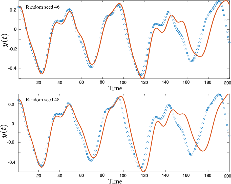
A small classical system () has limited accuracy with a NRSE (see Fig. 9). The same real sized quantum system obtains better results () as shown in Fig. 10 due to the larger size of its Hilbert space and larger number of available output quantities. It should be noted that here we consider a system in the strongly interacting regime, to obtain non-classical correlations. We have also neglected feedback caused by the process of measuring the quantum system, which implies the use of many copies of the system as considered in Ref. [10].
As a consistency check, let us now take our quantum reservoir in the regime , where the hopping between the sites is weaker than the decay rate . In this regime the quantum entanglement is suppressed and thus we lose the advantage of using the quantum reservoir, see Fig. 11.
References
- [1] Y. LeCun, Y. Bengio, and G. Hinton, Nature (London) 521, 436 (2015).
- [2] H. Jaeger and H. Haas, Science 304, 78 (2004).
- [3] W. Maass, T. Natschlager, and H. Markram, Neural Computation 14, 2531 (2002), https://doi.org/10.1162/089976602760407955 .
- [4] P. Enel, E. Procyk, R. Quilodran, and P. F. Dominey, PLoS Computational Biology 12, e1004967 (2016).
- [5] M. Lukoševičius and H. Jaeger, Computer Science Review 3, 127 (2009).
- [6] M. Lukoševičius, “A practical guide to applying echo state networks,” in Neural Networks: Tricks of the Trade: Second Edition, edited by G. Montavon, G. B. Orr, and K.-R. Müller (Springer Berlin Heidelberg, Berlin, Heidelberg, 2012) pp. 659–686.
- [7] L. Larger, A. Baylón-Fuentes, R. Martinenghi, V. S. Udaltsov, Y. K. Chembo, and M. Jacquot, Physical Review X 7, 011015 (2017).
- [8] D. Brunner, M. C. Soriano, C. R. Mirasso, and I. Fischer, Nature Communications 4, 1364 (2013).
- [9] L. Appeltant, M. C. Soriano, G. van der Sande, J. Danckaert, S. Massar, J. Dambre, B. Schrauwen, C. R. Mirasso, and I. Fischer, Nature Communications 2, 468 (2011).
- [10] K. Fujii and K. Nakajima, Physical Review Applied 8, 024030 (2017), arXiv:1602.08159 [quant-ph] .
- [11] K. Vandoorne, P. Mechet, T. van Vaerenbergh, M. Fiers, G. Morthier, D. Verstraeten, B. Schrauwen, J. Dambre, and P. Bienstman, Nature Communications 5, 3541 (2014).
- [12] J. Torrejon, M. Riou, F. A. Araujo, S. Tsunegi, G. Khalsa, D. Querlioz, P. Bortolotti, V. Cros, K. Yakushiji, A. Fukushima, H. Kubota, S. Yuasa, M. D. Stiles, and J. Grollier, Nature 547, 428 (2017).
- [13] http://www.neural-forecasting-competition.com/NN3/index.htm.
- [14] F. Schürmann, K. Meier, and J. Schemmel, in Advances in Neural Information Processing Systems 17, edited by L. K. Saul, Y. Weiss, and L. Bottou (MIT Press, 2005) pp. 1201–1208.
- [15] C. Du, F. Cai, M. A. Zidan, W. Ma, S. H. Lee, and W. D. Lu, Nature Communications 8, 2204 (2017).
- [16] D. Kudithipudi, Q. Saleh, C. Merkel, J. Thesing, and B. Wysocki, Frontiers in Neuroscience 9, 502 (2016).
- [17] Y. Paquot, F. Duport, A. Smerieri, J. Dambre, B. Schrauwen, M. Haelterman, and S. Massar, Scientific Reports 2, 287 (2012), arXiv:1111.7219 .
- [18] L. Larger, M. C. Soriano, D. Brunner, L. Appeltant, J. M. Gutierrez, L. Pesquera, C. R. Mirasso, and I. Fischer, Opt. Express 20, 3241 (2012).
- [19] F. Duport, B. Schneider, A. Smerieri, M. Haelterman, and S. Massar, Optics Express 20, 22783 (2012), arXiv:1207.1619 [physics.optics] .
- [20] J. C. Coulombe, M. C. A. York, and J. Sylvestre, PLoS ONE 12, e0178663 (2017), arXiv:1704.06320 .
- [21] C. Fernando and S. Sojakka, in Advances in Artificial Life, edited by W. Banzhaf, J. Ziegler, T. Christaller, P. Dittrich, and J. T. Kim (Springer Berlin Heidelberg, Berlin, Heidelberg, 2003) pp. 588–597.
- [22] G. Tanaka, T. Yamane, J. Benoit Héroux, R. Nakane, N. Kanazawa, S. Takeda, H. Numata, D. Nakano, and A. Hirose, ArXiv e-prints , arXiv:1808.04962 (2018), arXiv:1808.04962 [cs.ET] .
- [23] Y. Shen, N. C. Harris, S. Skirlo, M. Prabhu, T. Baehr-Jones, M. Hochberg, X. Sun, S. Zhao, H. Larochelle, D. Englund, and M. Soljačić, Nature Photonics 11, 441 (2017), arXiv:1610.02365 [physics.optics] .
- [24] H. J. Caulfield and S. Dolev, Nature Photonics 4, 261 EP (2010).
- [25] I. S. Aranson and L. Kramer, Rev. Mod. Phys. 74, 99 (2002).
- [26] J. Keeling and N. G. Berloff, Phys. Rev. Lett. 100, 250401 (2008).
- [27] R. Labouvie, B. Santra, S. Heun, and H. Ott, Phys. Rev. Lett. 116, 235302 (2016).
- [28] P. M. Walker, L. Tinkler, D. V. Skryabin, A. Yulin, B. Royall, I. Farrer, D. A. Ritchie, M. S. Skolnick, and D. N. Krizhanovskii, Nature Communications 6, 8317 EP (2015), article.
- [29] N. Y. Kim, K. Kusudo, A. Löffler, S. Höfling, A. Forchel, and Y. Yamamoto, New Journal of Physics 15, 035032 (2013).
- [30] K. Winkler, O. A. Egorov, I. G. Savenko, X. Ma, E. Estrecho, T. Gao, S. Müller, M. Kamp, T. C. H. Liew, E. A. Ostrovskaya, S. Höfling, and C. Schneider, Phys. Rev. B 93, 121303 (2016).
- [31] V. G. Sala, D. D. Solnyshkov, I. Carusotto, T. Jacqmin, A. Lemaître, H. Terças, A. Nalitov, M. Abbarchi, E. Galopin, I. Sagnes, J. Bloch, G. Malpuech, and A. Amo, Phys. Rev. X 5, 011034 (2015).
- [32] C. E. Whittaker, E. Cancellieri, P. M. Walker, D. R. Gulevich, H. Schomerus, D. Vaitiekus, B. Royall, D. M. Whittaker, E. Clarke, I. V. Iorsh, I. A. Shelykh, M. S. Skolnick, and D. N. Krizhanovskii, Phys. Rev. Lett. 120, 097401 (2018).
- [33] J. J. Hopfield, Phys. Rev. 112, 1555 (1958).
- [34] C. Weisbuch, M. Nishioka, A. Ishikawa, and Y. Arakawa, Phys. Rev. Lett. 69, 3314 (1992).
- [35] A. Kavokin, J. J. Baumberg, G. Malpuech, and F. P. Laussy, Microcavities (Oxford University Press, Inc., New York, NY, USA, 2008).
- [36] I. Carusotto and C. Ciuti, Rev. Mod. Phys. 85, 299 (2013).
- [37] J. Kasprzak, M. Richard, S. Kundermann, A. Baas, P. Jeambrun, J. M. J. Keeling, F. M. Marchetti, M. H. Szymanska, R. Andre, J. L. Staehli, V. Savona, P. B. Littlewood, B. Deveaud, and L. S. Dang, Nature 443, 409 (2006).
- [38] A. Amo, J. Lefrère, S. Pigeon, C. Adrados, C. Ciuti, I. Carusotto, R. Houdré, E. Giacobino, and A. Bramati, Nature Physics 5, 805 (2009).
- [39] H. Deng, H. Haug, and Y. Yamamoto, Rev. Mod. Phys. 82, 1489 (2010).
- [40] D. Ballarini, M. De Giorgi, E. Cancellieri, R. Houdré, E. Giacobino, R. Cingolani, A. Bramati, G. Gigli, and D. Sanvitto, Nature Communications 4, 1778 EP (2013), article.
- [41] T. Gao, P. S. Eldridge, T. C. H. Liew, S. I. Tsintzos, G. Stavrinidis, G. Deligeorgis, Z. Hatzopoulos, and P. G. Savvidis, Phys. Rev. B 85, 235102 (2012).
- [42] A. Amo, T. C. H. Liew, C. Adrados, R. Houdré, E. Giacobino, A. V. Kavokin, and A. Bramati, Nature Photonics 4, 361 EP (2010).
- [43] T. Espinosa-Ortega and T. C. H. Liew, Physical Review Letters 114, 118101 (2015), arXiv:1408.6949 [cond-mat.dis-nn] .
- [44] H. Ohadi, A. Dreismann, Y. G. Rubo, F. Pinsker, Y. del Valle-Inclan Redondo, S. I. Tsintzos, Z. Hatzopoulos, P. G. Savvidis, and J. J. Baumberg, Phys. Rev. X 5, 031002 (2015).
- [45] Y. LeCun, L. Bottou, Y. Bengio, and P. Haffner, Proceedings of the IEEE 86, 2278 (1998).
- [46] N. Bobrovska, M. Matuszewski, K. S. Daskalakis, S. A. Maier, and S. Kéna-Cohen, ACS Photonics 5, 111 (2018).
- [47] G. Nardin, G. Grosso, Y. Léger, B. Pietka, F. Morier-Genoud, and B. Deveaud-Plédran, Nature Physics 7, 635 EP (2011), article.
- [48] M. Abbarchi, A. Amo, V. G. Sala, D. D. Solnyshkov, H. Flayac, L. Ferrier, I. Sagnes, E. Galopin, A. Lemaître, G. Malpuech, and J. Bloch, Nature Physics 9, 275 EP (2013).
- [49] P. Cilibrizzi, H. Sigurdsson, T. C. H. Liew, H. Ohadi, A. Askitopoulos, S. Brodbeck, C. Schneider, I. A. Shelykh, S. Höfling, J. Ruostekoski, and P. Lagoudakis, Phys. Rev. B 94, 045315 (2016).
- [50] M. Pieczarka, M. Syperek, L. Dusanowski, A. Opala, F. Langer, C. Schneider, S. Höfling, and G. Sek, Scientific Reports 7, 7094 (2017).
- [51] Q. Wang, Y. Li, and P. Li, in 2016 IEEE International Symposium on Circuits and Systems (ISCAS) (2016) pp. 361–364.
- [52] M. Milićević, T. Ozawa, P. Andreakou, I. Carusotto, T. Jacqmin, E. Galopin, A. Lemaître, L. L. Gratiet, I. Sagnes, J. Bloch, and A. Amo, 2D Materials 2, 034012 (2015).
- [53] P. A. Merolla, J. V. Arthur, R. Alvarez-Icaza, A. S. Cassidy, J. Sawada, F. Akopyan, B. L. Jackson, N. Imam, C. Guo, Y. Nakamura, B. Brezzo, I. Vo, S. K. Esser, R. Appuswamy, B. Taba, A. Amir, M. D. Flickner, W. P. Risk, R. Manohar, and D. S. Modha, Science 345, 668 (2014), http://science.sciencemag.org/content/345/6197/668.full.pdf .
- [54] D. Li, M. Han, and J. Wang, IEEE Transactions on Neural Networks and Learning Systems 23, 787 (2012).
- [55] R. Lyon, in ICASSP ’82. IEEE International Conference on Acoustics, Speech, and Signal Processing, Vol. 7 (1982) pp. 1282–1285.
- [56] D. Verstraeten, B. Schrauwen, D. Stroobandt, and J. V. Campenhout, Information Processing Letters 95, 521 (2005), applications of Spiking Neural Networks.
- [57] L.-M. Duan, G. Giedke, J. I. Cirac, and P. Zoller, Phys. Rev. Lett. 84, 2722 (2000).
- [58] R. Simon, Phys. Rev. Lett. 84, 2726 (2000).