Plato: Approximate Analytics over Compressed Time Series with Tight Deterministic Error Guarantees

Chunbin Lin Affiliation: University of California, San Diego email: chunbinlin@cs.ucsd.edu , Etienne Boursier Affiliation: ENS Paris-Saclay email: eboursie@ens-paris-saclay.fr and Yannis Papakonstantinou Affiliation: University of California, San Diego email: yannis@cs.ucsd.edu

Abstract.

Plato provides fast approximate analytics on time series, by precomputing and storing compressed time series. Plato’s key novelty is the delivery of tight deterministic error guarantees for time series analytics. Plato evaluates any time series expression composed by the linear algebra operators over vectors, along with arithmetic operators. This large scope of possible expressions includes common use cases such as correlation and cross-correlation expressions. Each time series is segmented either by fixed-length segmentation or by (a usually more effective) variable-length segmentation. Each segment is compressed by an estimation/compression function that approximates the actual values and is coming from a user-chosen function family, as taught by many prior works. The novelty is that Plato associates to each segment 1 to 3 (depending on the case) precomputed error measures and, using them, Plato computes tight deterministic error guarantees for analytics over the compressions.

Importantly, some compression families lead to much better deterministic error guarantees. This work identifies two broad estimation function family groups (Vector Space (VS) and Linear Scalable Family (LSF)), which lead to theoretically and practically high-quality guarantees, even for expressions (eg correlation) that combine multiple time series that have been independently compressed and may, thus, use misaligned segmentations. The theoretical aspect of “high quality” is crisply captured by the Amplitude Independence (AI) property: An AI guarantee does not depend on the amplitude of the involved time series, even when we combine multiple time series. The experiments on four real-life datasets showed that when the novel AI guarantees were applicable, the approximate query results were certified to be very close (typically $1\%$ ) to the true results.

1. Introduction

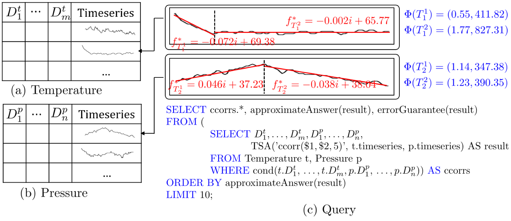
Refer to caption — Figure 1. Example of SQL query using the time series analytic (TSA) UDF.

Attention to time series analytics is bound to increase in the IoT era as cheap sensors can now deliver vast volumes of many types of measurements. The size of the data is also bound to increase. E.g., an IoT-ready oil drilling rig produces about $8$ TB of operational data in one day. ¹¹ 1 https://wasabi.com/storage-solutions/internet-of-things/ One way to solve this problem is to increase the expense in computing and storage in order to catch up. However, in many domains, the data size increase is expected to outpace the increase of computing abilities, thus making this approach unattractive (Galakatos et al., 2017; Chaudhuri et al., 2017). Another solution is approximate analytics over compressed time series.

	function	error guarantees on	AI	Tight	error guarantees on	AI	Tight
	family	aligned time series			misaligned time series
$Sum(\bm{T_{1}\times T_{2}})$	ANY $\setminus$ VS	$\sum\limits_{i=1}^{k}\Big(\\|\varepsilon_{T_{1}^{i}}\\|_{2}\times\\|\varepsilon_{T_{2}^{i}}\\|_{2}\Big)$	✗	✓	$\;\;\sum_{i=1}^{k_{1}}\Big(\\|\varepsilon_{T_{1}^{i}}\\|_{2}\times(\sum_{j\in\Pi_{T_{2},[a_{1}^{i},b_{1}^{i}]}}\\|f_{T_{2}^{j}}\\|_{2}^{2})^{\frac{1}{2}}\Big)$	✗	✓
		$+\sum\limits_{i=1}^{k}\Big(\\|\varepsilon_{T_{1}^{i}}\\|_{2}\times\\|f_{T_{2}^{i}}\\|_{2}\Big)$			$+\sum_{i=1}^{k_{2}}\Big(\\|\varepsilon_{T_{2}^{i}}\\|_{2}\times(\sum_{j\in\Pi_{T_{1},[a_{2}^{i},b_{2}^{i}]}}\\|f_{T_{1}^{j}}\\|_{2}^{2})^{\frac{1}{2}}\Big)$
		$+\sum\limits_{i=1}^{k}\Big(\\|\varepsilon_{T_{2}^{i}}\\|_{2}\times\\|f_{T_{1}^{i}}\\|_{2}\Big)$			$+\sum\limits_{[a,b]\in OPT(L_{T_{1}},L_{T_{2}})}\Big(\big(\sum_{i\in\Pi_{T_{1},[a,b]}}\\|\varepsilon_{T_{1}^{i}}\\|_{2}^{2}\big)^{\frac{1}{2}}$
	VS $\setminus$ LSF	$\sum\limits_{i=1}^{k}\Big(\\|\varepsilon_{T_{1}^{i}}\\|_{2}\times\\|f_{T_{2}^{i}}\\|_{2}\Big)$	✓	✓	$\;\;\;\;\;\;\;\;\;\;\;\;\;\;\;\;\;\;\;\;\;\;\;\times\big(\sum_{i\in\Pi_{T_{2},[a,b]}}\\|\varepsilon_{T_{2}^{i}}\\|_{2}^{2}\big)^{\frac{1}{2}}\Big)$
	LSF				$\;\;\sum_{i=1}^{k_{1}}\Big(\\|\varepsilon_{T_{1}^{i}}\\|_{2}\times\\|\bm{f_{T_{2}}\|_{[a_{1}^{i},b_{1}^{i}]}-f^{*}_{T_{1}^{i}}}\\|_{2}\Big)$	✓	✓
					$+\sum_{i=1}^{k_{2}}\Big(\\|\varepsilon_{T_{2}^{i}}\\|_{2}\times\\|\bm{f_{T_{1}}\|_{[a_{2}^{i},b_{2}^{i}]}-f^{*}_{T_{2}^{i}}}\\|_{2}\Big)$
					$+\sum\limits_{[a,b]\in OPT(L_{T_{1}},L_{T_{2}})}\Big(\big(\sum_{i\in\Pi_{T_{1},[a,b]}}\\|\varepsilon_{T_{1}^{i}}\\|_{2}^{2}\big)^{\frac{1}{2}}$
					$\;\;\;\;\;\;\;\;\;\;\;\;\;\;\;\;\;\;\;\;\;\;\;\times\big(\sum_{i\in\Pi_{T_{2},[a,b]}}\\|\varepsilon_{T_{2}^{i}}\\|_{2}^{2}\big)^{\frac{1}{2}}\Big)$
$Sum(\bm{T_{1}+T_{2}})$	ANY	$\sum\limits_{i=1}^{k}(\gamma_{T_{1}^{i}}+\gamma_{T_{2}^{i}})$	✓	✓	$\sum\limits_{i=1}^{k_{1}}\gamma_{T_{1}^{i}}+\sum\limits_{j=1}^{k_{2}}\gamma_{T_{2}^{j}}$	✓	✓
$Sum(\bm{T_{1}-T_{2}})$

Table 1. Error guarantees for the time series analytic (TSA)

Sum(T_{1}\diamond T_{2})

where

\diamond\in\{\times,+,-\}

on both aligned and misaligned time series compressed by estimation functions in different families. We assume

T_{1}

and

T_{2}

have

k_{1}

and

k_{2}

segments respectively. In the aligned case, we have

k_{1}=k_{2}=k

OPT(L_{T_{1}},L_{T_{2}})

is the optimal segment combination returned by the algorithm OS in Section 4.2.1

Example 0.

Consider the database in Figure 1, which has a Temperature table and a Pressure table. Each table contains (i) one Timeseries column containing time series data, as a UDT (Eisenberg and Melton, 2002) and (ii) several other “dimension" attributes $D$ , such as the identification and other properties of the sensors that delivered the time series. The Plato SQL query in Figure 1(c) “returns the top-10 temperature/pressure 5-second cross-correlation scores among all the (temperature, pressure) pairs satisfying a (not detailed in the example) condition cond() over the dimension attributes”. The Time Series Analytic (TSA) function evaluates the time series expression ’CCorr(t.timeseries, p.timeseries, 5)’. (The $1 is instantianted by the second argument of the TSA and similarly for the $2.) In SQL, the result is a string concatenation of the approximate answer and the error guarantee. The functions approximateAnswer and errorGuarantee extract the respective pieces. The filtering conditions in the WHERE clause have no effects to our techniques as a time series is either completely selected or completely pruned. For the case where only a part of the time series is chosen, see the Restriction operator in Section 2. Furthermore, this work is orthogonal to how to assemble the time series values from plain relational tables that have no time series type.

Note, instead of using the cross-correlation expression CCorr the user could use more basic functions to write out the definition of cross-correlation, as shown in Table 4. The result would be the same. Either way, computing the accurate cross-correlations would cost more than $10$ minutes, in the experimental setting of Figure 10, in Experiments. However, Plato reduces the runtime to within one second by computing the approximate correlations. It also delivers deterministic error guarantees, which means the error guarantees have a $100\%$ confidence.

Deterministic error guarantees vs. probabilistic error guarantees. Both deterministic error guarantees (Cormode et al., 2005; Greenwald and Khanna, 2001; Manku et al., 1998; Potti and Patel, 2015; Lazaridis and Mehrotra, 2001; Poosala et al., 1996) and probabilistic error guarantees (Chaudhuri et al., 2007; Sidirourgos et al., 2011; Pansare et al., 2011; Agarwal et al., 2013) are widely utilized in approximate query processing. We follow the deterministic error guarantees direction. Section 5.2 compares deterministic and probabilistic guarantees.

The success of approximate querying on IoT time series data is based on an important beneficial property of time series data: the points in the sequence of values normally depend on the previous points and exhibit continuity. For example, a temperature sensor is very unlikely to report a 100 degrees increase within a second. Therefore, in the signal processing and data mining communities (Keogh et al., 2001a; Keogh, 1997; Faloutsos et al., 1994; Chan and Fu, 1999), time series data is usually modeled and compressed by continuous functions in order to reduce its size. For instance, the Piecewise Aggregate Approximation (PAA) (Keogh et al., 2001a) and the Piecewise Linear Representation (PLR) (Keogh, 1997) adopt polynomial functions (0-degree in PAA and 1-degree in PLR) to compress the time series; (Pan et al., 2017) uses Gaussian functions; (Tobita, 2016) applies natural logarithmic functions and natural exponential functions to compress time series. Plato is open to any existing time series compression technique, since there is no one-size-fits-all compression function family that can best model all kinds of time series data. For example, polynomials and ARMA models are better at modeling data from physical processes such as temperature (Mei and Moura, 2017; Choi, 2012), while Gaussian functions are better for modeling relatively randomized data (Kim, 2003) such as stock prices. How to choose the best compression function family has been widely studied in prior work (Philo, 1997; Wiscombe and Evans, 1977; Denison et al., 1998; Kovács et al., 2002) and recent efforts even attempt to automate the process (Kumar et al., 2015). In this paper, the choice of compression function family is made by the user. Plato will deliver the best guarantees, given the chosen family.

Architecture. Figure 2 shows the high-level architecture. During insertion time, the provided time series is compressed. In particular, a compression function family (e.g., 2nd-degree polynomials) is chosen by the user. Internally, in a simple version, each time series is segmented (partitioned) first in equal lengths. Then, for each segment the system finds the best estimation function, which is the member of the function family that best approximates the values in this segment. The most common definition of “best” is the minimization of the reconstruction error, i.e., the minimization of the Euclidean distance between the original and the estimated values. This is also the definition that Plato assumes. The compressed database stores the parameters of the estimation function for each segment, which take much less space than the original time series data. In the more sophisticated version, segmentation and estimation are mingled together (Koski et al., 1995; Keogh et al., 2001b) to achieve better compression. The result is that the time series is partitioned into variable-length segments.

Consequently, given a query $q$ with Time Series Analytics (TSA) UDF calls, the database computes quickly an approximate answer for each TSA call by using the compressed data.

Example 0.

Consider a room temperature time series $T_{1}$ and an air pressure time series $T_{2}$ in Figure 1 and consider the TSA(‘Ccorr( $T_{1},T_{2}$ , $60$ )’, $T_{1}$ , $T_{2}$ ) where ‘Ccorr( $T_{1},T_{2},60$ )’ refers to the 60-seconds cross-correlation of $T_{1}$ and $T_{2}$ (see definition in Table 4). Both $T_{1}$ and $T_{2}$ have $600$ data points at 1-second resolution and are segmented by variable length segmentation methods and compressed by PLR (1-degree polynomial functions). The precise answer is $0.303$ . But instead of accessing the $1200$ ( $600\times 2$ ) original data points, Plato produces the approximate answer $0.300$ (error is $0.003$ ) by accessing just the function parameters ( $-0.072,69.38$ ), ( $-0.002,65.77$ ) for $T_{1}$ and ( $-0.046,37.23$ ), ( $-0.038,38.04$ ) for $T_{2}$ in the compressed database.²² 2 Due to reasons relating to computation efficiency, as explained in Section 4.2.2, Plato does not actually store the parameters ( $-0.072,69.38$ ), ( $-0.002,65.77$ ) and ( $-0.046,37.23$ ), ( $-0.038,38.04$ ) in their standard basis but rather it stores coefficients in an orthonormal basis.

The well-known downside of approximate querying is that errors are introduced. When the example’s user receives the approximate answer $0.300$ she cannot tell how far this answer is from the true answer, i.e., the precise answer. The novelty of Plato is the provision of tight (i.e., lower bound) deterministic error guarantees for the answers, even when the time series expressions combine multiple series. In the Example 2, Plato guarantees that the true answer is within $\pm 0.0032$ of the approximate answer $0.300$ with $100\%$ confidence. (Indeed, $0.303$ is within $\pm 0.0032$ of $0.300$ .)

Scope of Time Series Expressions. Plato supports the time series analytic expressions formally defined in Table 3 (Section 2). They are composed of vector operators ( $\mathbf{+}$ , $\mathbf{-}$ , $\mathbf{\times}$ , Shift), arithmetic operators, the aggregation operator Sum that turns its input vector into a scalar, and the Constant operator that turns its input scalar into a vector. As such, Plato queries can express not only statistics that involve one time series (eg, average, variance, and n-th moment) but also statistics that involve multiple time series, such as correlation and cross-correlation.

Goal of Plato. The goal of Plato is to provide tight deterministic error guarantees for the time series expressions. It is challenging as each time series is segmented and compressed individually before the queries arrive, which results in (i) time series segmentations are misaligned, and (ii) different compression functions are utilized in different time series. To solve the challenge, Plato computes error measures of Table 2 during the compression time for each time series segment. Figure 1 shows the error measures $\Phi$ (in blue) for each segment of the example. With the help of the error measures, no matter whether a time series is compressed by trigonometric functions or polynomial functions or some other family, Plato is able to give tight deterministic error guarantees for queries involving the compressed time series.

Error measures	Comments
$\\|\varepsilon_{T}\\|_{2}=\sqrt{\sum_{i=a}^{b}(T[i]-f^{*}_{T}(i))^{2}}$	$L_{2}$ -norm of the estimation errors
$\\|f_{T}\\|_{2}=\sqrt{\sum_{i=a}^{b}(f^{*}_{T}(i))^{2}}$	$L_{2}$ -norm of the estimated values
$\gamma_{T}=\|\sum_{i=a}^{b}T[i]-\sum_{i=a}^{b}f^{*}_{T}(i)\|$	Absolute reconstruction error

Table 2. Error measures stored for a time series segment

T

running from

a

b

and approximated with the estimation function

f^{*}_{T}

Function Family Groups Producing Practical Error Guarantees. Plato produces tight error guarantees, for any function family that may have been used in the compression. In addition, our theoretical and experimental analysis identifies which families lead to high quality guarantees.

The formulas of Table 1 provide error guarantees for characteristic, simple expressions and exhibit the difference in guarantee quality. Any other expression, e.g., the statistics of Table 4, are also given error guarantees by composing the error measures and guarantees of their subexpressions (as shown in the paper) and the same quality characterizations apply to them inductively.

This is how to interpret the results of Table 1: Three function family groups have been identified: (1) The Linear Scalable Family group (LSF), (2) the Vector Space (VS), which includes the LSF and (3) ANY, which, according to its name, includes everything. Given the function family $\mathds{F}$ used in the compression, we first categorize $\mathds{F}$ in one of LSF or VS/LSF (i.e., VS excluding LSF) or ANY/VS. For example, if $\mathds{F}$ is the 2-degree polynomials, then $\mathds{F}$ belongs to LSF. See Figure 3 for other examples. Next, we consider whether the segments of the involved compressed time series are aligned or misaligned and finally we look at the error guarantee formula for the expression.

Amplitude Independence (AI). The specifics of interpreting the table’s results and the specifics of their efficient computation require the detailed discussion of the paper. Nevertheless, a clear and general high level lesson about the practicality of the error guarantees emerges from the table’s summary: Some function families allow for much higher quality error guarantees than other function families. The typical characteristic of “higher quality” is Amplitude Independence (AI). If an error guarantee is AI, then it is not influenced by the $\|f_{T}\|_{2}$ measure, i.e., it is not affected by the amplitude of the values of the estimation functions and, thus, it is not affected from the amplitude of the original data. An AI error guarantee is only affected by the reconstruction errors caused by the estimation functions, which intuitively implies that AI error guarantees are close to the actual error.

Tight Error Guarantees . These guarantees are tight in the following sense. Given (a) the function family categorization into LSF, VS/LSF or ANY/VS and (b) segments with the error measures of Table 2, the formula provided by Table 1 produces an error guarantee that is as small as possible. That is, for this superfamily and for the given error measures, any attempt to create a better (i.e., smaller) error guarantee will fail because there are provably time series and at least one time series analytics expression where the true error is exactly as large as the error guarantee.

The experimental results, where we tried data sets with different characteristics and different compression methods, verified the above intuition: AI error guarantees were order(s) of magnitude smaller than their amplitude dependent counterparts. Particularly interesting are the analytics that combine multiple vectors by vector multiplication (eg, cross-correlation). Then the amplitude independence of the error guarantees does not apply to all families and, thus, this study says that one should be careful in the choice, if error guarantees are needed.

The contributions are summarized as follows.

•

We deliver tight deterministic error guarantees for a wide class of analytics over compressed time series. The key challenge is analytics (e.g., correlation and cross-correlation) that combine multiple time series but it is not known in advance which time series may be combined. Thus, each time series has been compressed individually, much before a query arrives. The reconstruction errors of the individual time series’ compressions cannot provide, by themselves, decent guarantees for queries that multiply time series. To make the problem harder, time series segmentations are generally misaligned.³³ 3 Misalignment happens because the most effective compressions use variable length segmentations. But even if the segmentations were fixed length, queries such as cross-corellation and cross-autocorellation time shift one of their time series, thus producing misalignment with the second time series.
•

The provided guarantees apply regardless of the specifics of the segmentation and estimation function family used during the compression, thus making the provided deterministic error guarantees applicable to any prior work on segment-based compression (eg, variable-sized histograms etc). The only requirement is the common assumption that the estimation function minimizes the Euclidean distance between the actual values and the estimates.
•

We identify broad estimation function family groups (namely, the already defined Vector Space family and the presently defined Linear Scalable Family) that lead to theoretically and practically high quality guarantees. The theoretical aspect of high quality is crisply captured by the Amplitude Independence (AI) property. Furthermore, the error guarantees are computed very efficiently, in time proportional to the number of segments.
•

The results broadly apply to analytics involving composition of the typical operators, which is powerful enough to express common statistics, such as variance, correlation, cross-correlation and other in any time range.
•

We conduct an extensive empirical evaluation on four real-life datasets to evaluate the error guarantees provided by Plato and the importance of the VS and LSF properties on error estimation. The results show that the AI error guarantees are very narrow - thus, practical. Furthermore, we compare to sampling-based approximation and show experimentally that Plato delivers deterministic (100% confidence) error guarantees using fewer data than it takes to produce probabilistic error guarantees with 95% and 99% confidence via sampling.

2. Time Series and Expressions

Time Series Analytic (TSA)
Q	$\rightarrow$	Ar
Arithmetic Expression (Ar)
Ar	$\rightarrow$	literal value in $R$
	\|	Ar $\otimes$ Ar	where $\otimes\in\{+,-,\times,\div,\sqrt{~}\}$
	\|	Agg
Aggregation Expression (Agg)
Agg	$\rightarrow$	Sum( $\bm{T},a^{\prime},b^{\prime}$ )	$\sum_{i=a^{\prime}}^{b^{\prime}}\bm{T}[i]$ , where $[a^{\prime},b^{\prime}]\subseteq[a,b]$
Time Series Expression (TSE)
$\bm{T}$	$\rightarrow$	input time series
	\|	Constant $(\upsilon,a,b)$	$(a,b,[\underbrace{\upsilon,\upsilon,...,\upsilon}_{b-a+1}])$
	\|	Shift $(\bm{T},k)$	$(a+k,b+k,[\bm{T}[a],...,\bm{T}[b]])$
	\|	$\bm{T_{1}+T_{2}}$	$(a,b,[\bm{T_{1}}[a]+\bm{T_{2}}[a],...,\bm{T_{1}}[b]+\bm{T_{2}}[b]])$
	\|	$\bm{T_{1}-T_{2}}$	$(a,b,[\bm{T_{1}}[a]-\bm{T_{2}}[a],...,\bm{T_{1}}[b]-\bm{T_{2}}[b]])$
	\|	$\bm{T_{1}\times T_{2}}$	$(a,b,[\bm{T_{1}}[a]\times\bm{T_{2}}[a],...,\bm{T_{1}}[b]\times\bm{T_{2}}[b]])$

Table 3. Grammar of time series analytic (TSA). Let

\bm{T}_{1}=(a_{1},b_{1},[\bm{T_{1}}[a_{1}],...,\bm{T_{1}}[b_{1}]])

and

\bm{T}_{2}=(a_{2},b_{2},[\bm{T_{2}}[a_{2}],...,\bm{T_{2}}[b_{2}]])

be the input time series in the time series expressions,

a=\max(a_{1},a_{2})

and

b=\min(b_{1},b_{2})

Time Series A time series $\bm{T}=(a,b,[\bm{T}[a],\bm{T}[a+1],...,\bm{T}[b]])$ , $a\in N$ , $b\in N$ , is a sequence of data points $[\bm{T}[a],\bm{T}[a+1],...,\bm{T}[b]]$ observed from start time $a$ to end time $b$ ( $a,b\in N$ ). Following the assumptions in (Morse and Patel, 2007; Chen and Ng, 2004; Vlachos et al., 2002) we assume that time is discrete and the resolution of any two time series is the same. Equivalently, we say $\bm{T}$ is fully defined in the integer time domain $[a,b]$ . We assume a domain $[1,n]$ is the global domain meaning that all the time series are defined within subsets of this domain. When the domain of a time series $\bm{T}$ is implied by the context, then $\bm{T}$ can be simplified as $\bm{T}=[\bm{T}[a],\bm{T}[a+1],...,\bm{T}[b]]$ .

Example 0.

Assume the global domain is $[1,100]$ . Consider two time series $\bm{T}_{1}=(1,5,[61.52,59.54,58.64,59.36,$ $60.44])$ and $\bm{T}_{2}=(3,6,[1.02,1.03,1.02,1.02])$ . Then $\bm{T}_{1}$ and $\bm{T}_{2}$ are fully defined in domains [1,5] and [3,6] respectively. $\bm{T}_{2}[4]=1.03$ refers to the $2^{nd}$ data point of $\bm{T}_{2}$ at the $4$ -th position in the global domain.

TSA Expression	Definition	Equivalent TSA Expression	Usage of error measures
Average $\mu_{T_{1}}$ ‘ $\mu$ ( $T_{1}$ )’	$\dfrac{1}{b_{1}-a_{1}+1}(\sum\limits_{i=a_{1}}^{b_{1}}T_{1}[i])$	$\dfrac{1}{b_{1}-a_{1}+1}$ (Sum( $\bm{T_{1}}$ ))	$\gamma_{T_{1}}$
Standard Deviation $\sigma_{T_{1}}$ ‘ $\sigma$ ( $T_{1}$ )’	$\sqrt{\frac{1}{b_{1}-a_{1}+1}\Big(\sum\limits_{i=a_{1}}^{b_{1}}(T_{1}[i]-\mu_{T_{1}})^{2}\Big)}$	$\sqrt{\frac{1}{b_{1}-a_{1}+1}\times Sum(\bm{T_{1}-}\textsf{Constant}(\mu_{T_{1}}))}$	$\gamma_{T_{1}}$
Correlation $r_{(T_{1},T_{2})}$ ‘Corr( $T_{1}$ , $T_{2}$ )’	$\dfrac{\sum\limits_{i=max(a_{1},a_{2})}^{min(b_{1},b_{2})}\Big((T_{1}[i]-\mu_{T_{1}})(T_{2}[i]-\mu_{T_{2}})\Big)}{\sigma_{T_{1}}\times\sigma_{T_{2}}}$	$\dfrac{Sum\Big((\bm{T_{1}-}\textsf{Constant}(\mu_{T_{1}}))\bm{\times}(\bm{T_{2}-}\textsf{Constant}(\mu_{T_{2}}))\Big)}{\sigma_{T_{1}}\times\sigma_{T_{2}}}$	$\\|\varepsilon_{T_{1}}\\|_{2}$ , $\\|f_{T_{1}}\\|_{2}$ , $\gamma_{T_{1}}$ , $\\|\varepsilon_{T_{2}}\\|_{2}$ , $\\|f_{T_{2}}\\|_{2}$ , $\gamma_{T_{2}}$
Cross-correlation $r_{(T_{1},T_{2},m)}$ ‘CCorr( $T_{1}$ , $T_{2}$ , $m$ )’	$\dfrac{\sum\limits_{i=max(a_{1},a_{2}+m)}^{min(b_{1},b_{2}+m)}\Big((T_{1}[i]-\mu_{T_{1}})(T_{2}[i+m]-\mu_{T_{2}})\Big)}{\sigma_{T_{1}}\times\sigma_{T_{2}}}$	$\dfrac{Sum\Big((\bm{T_{1}-}\textsf{Constant}(\mu_{T_{1}}))\bm{\times}(Shift(\bm{T_{2}},m)\bm{-}\textsf{Constant}(\mu_{T_{2}}))\Big)}{\sigma_{T_{1}}\times\sigma_{T_{2}}}$	$\\|\varepsilon_{T_{1}}\\|_{2}$ , $\\|f_{T_{1}}\\|_{2}$ , $\gamma_{T_{1}}$ , $\\|\varepsilon_{T_{2}}\\|_{2}$ , $\\|f_{T_{2}}\\|_{2}$ , $\gamma_{T_{2}}$
Auto-correlation $r_{(T_{1},m)}$ ‘ACorr( $T_{1}$ , $m$ )’	$\dfrac{\sum\limits_{i=a_{1}+m}^{b_{1}}\Big((T_{1}[i]-\mu_{T_{1}})(T_{1}[i+m]-\mu_{T_{1}})\Big)}{\sigma_{T_{1}}^{2}}$	$\dfrac{Sum\Big((\bm{T_{1}-}\textsf{Constant}(\mu_{T_{1}}))\bm{\times}(Shift(\bm{T_{1}},m)\bm{-}\textsf{Constant}(\mu_{T_{1}}))\Big)}{\sigma_{T_{1}}\times\sigma_{T_{1}}}$	$\\|\varepsilon_{T_{1}}\\|_{2}$ , $\\|f_{T_{1}}\\|_{2}$ , $\gamma_{T_{1}}$

Table 4. Example TSA’s for common statistics. Let

\bm{T}_{1}=(a_{1},b_{1},[\cdots])

and

\bm{T}_{2}=(a_{2},b_{2},[\cdots])

be the input time series in the time series analytic.

Time Series Analytic (TSA) Expressions Table 3 shows the formal definition of the time series analytic (called TSA). The TSAs supported are expressions composed of linear algebra operators and arithmetic operators. Typically, the TSA has subexpressions that compose one or more linear algebra operators over multiple time series vectors as defined below.

•

Given a numeric value $\upsilon$ and two integers $a$ and $b$ , Constant $(\upsilon,a,b)=(a,b,[\upsilon,...,\upsilon])$ . For example, Constant( $1.6,3,5$ ) produces $(3,5,[1.6,1.6,1.6])$ .
•

Given a time series $\bm{T}=(a,b,[\bm{T}[a],...,\bm{T}[b]])$ and an integer value $k$ , Shift( $\bm{T},k$ )= $(a+k,b+k,[\bm{T}[a],...,\bm{T}[b]])$ . Notice Shift( $\bm{T},k$ ) $[i+k]$ = $\bm{T}[i]$ for all $a\leq i\leq b$ . Figure 4(a) visualizes the Shift operator. Consider the time series $\bm{T}=(1,3,[1.8,1.6,1.6])$ , then Shift( $\bm{T},6$ ) is $(7,9,$ $[1.8,1.6,1.6])$ .
•

Given two time series $\bm{T}_{1}=(a_{1},b_{1},[\bm{T}_{1}[a_{1}],...,\bm{T}_{1}[b_{1}]])$ and $\bm{T}_{2}=(a_{2},b_{2},[\bm{T}_{2}[a_{2}],...,\bm{T}_{2}[b_{2}]])$ , $\bm{T_{1}\times T_{2}}=(a,b,[\bm{T}_{1}[a]$ $\times\bm{T}_{2}[a],$ $...,\bm{T}_{1}[b]\times\bm{T}_{2}[b]])$ where $a=max(a_{1},a_{2})$ and $b=min(b_{1},b_{2})$ . ⁴⁴ 4 Setting $a=max(a_{1},a_{2})$ and $b=min(b_{1},b_{2})$ ensures all the data points in $\bm{T_{1}\times T_{2}}$ are defined. For example, given $\bm{T}_{1}=(1,2,[3.3,$ $3.5])$ and $\bm{T}_{2}=(1,2,[1.0,1.2])$ then $\bm{T_{1}\times T_{2}}=(1,2,[3.3,4.2])$ . Similarly, we define $\bm{T_{1}+T_{2}}$ and $\bm{T_{1}-T_{2}}$ .

A time series analytic (TSA) is an arithmetic expression of the form $Arr_{1}\otimes Arr_{2}\otimes\ldots Arr_{n}$ , where $\otimes$ are the standard arithmetic operators ( $+,-,\times,\div,\sqrt{~}$ ) and $Arr_{i}$ is either an arithmetic literal or an aggregation over a time series expression. An aggregation expression Sum $(\bm{T},a^{\prime},b^{\prime})$ computes the summation of the data points of $T$ in the domain $[a^{\prime},b^{\prime}]$ , i.e., Sum $(\bm{T},a^{\prime},b^{\prime})$ = $\sum_{i=a^{\prime}}^{b^{\prime}}\bm{T}[i]$ where $\bm{T}$ can be an input time series or a derived time series computed by time series expressions (TSEs). ⁵⁵ 5 Note that, when the time series expressions involve time shifting, we assume that the aggregation will only operator in the valid data points, that is the data points in the defined range. When the bounds of $a^{\prime}$ and $b^{\prime}$ are implied from the context, we simplify $Sum(\bm{T},a^{\prime},b^{\prime})$ to $Sum(\bm{T})$ .

3. Internal, Compressed Time Series Representation

When a user inserts a time series into the database, Plato physically stores the compressed time series representation instead of the raw time series. More precisely, the user provides (i) a time series $T$ , (ii) the identifier of a segmentation algorithm, which is chosen from a list provided by Plato, and (iii) the identifier of a function family, which is selected from a list provided by Plato. Internally, Plato uses the chosen segmentation algorithm and the chosen compression function family to partition $T$ into a list of disjoint segments $T^{1},...,T^{n}$ . For each segment $T^{i}=(a,b,[T^{i}[a],...,T^{i}[b]])$ , instead of storing its original data points $[T^{i}[a],...,T^{i}[b]]$ , Plato stores a compressed segment representation $\tilde{T^{i}}=(a,b,\tilde{f^{*}_{T}},\Phi(T))$ , where $a$ is the start position, $b$ is the end position, $\tilde{f^{*}_{T}}$ is the function representation of $f^{*}_{T}$ , where $f^{*}_{T}$ is the estimation function chosen from the identified function family and $\Phi(T)$ is a set of (two to three depending on the function family) error measures.

Overall, for a time series $T$ , Plato physically stores (i) the list $L_{T}$ =( $\tilde{T^{1}},...,\tilde{T^{n}}$ ), and (ii) one token (which can simply be an integer) as the function family identifier. ⁶⁶ 6 It is not necessary for Plato to physically store a token for the segmentation algorithm identifier as the time series stored in Plato has been partitioned already.

We comment on the prior state-of-the-art segmentation / compression algorithms that Plato uses in Appendix A. Next, we introduce the selection of the estimation function and the computation of error measures.

3.1. Estimation Function Selection

Choosing an estimation function for a time series segment has two steps: (i) user identifies the function family, and (ii) Plato selects the best function in the family, i.e., the function that minimizes the Euclidean distance between the original values and the estimated values produced by the function.

Step 1: Function family selection. Table 8 gives example function family identifiers, which the user may select, and the corresponding function expressions. For example, $\tau$ =“ $p_{2}$ ” means that the chosen function family is the “second-degree polynomial function family” and the corresponding function family expression is $\{ax^{2}+bx+c|a,b,c\in R\}$ .

Step 2: Estimation function selection. Any function $f$ in the chosen function family $\mathds{F}$ is a candidate estimation function. Following the prior work (Lazaridis and Mehrotra, 2003; Aghabozorgi et al., 2015), Plato selects the candidate estimation function that minimizes the Euclidean distance between the original values and the estimated values produced by the function to be the final estimation function. More precisely,

(1)

\displaystyle f^{*}_{T}=\arg\min_{f\in\mathds{F}}\Big(\sum_{i=a}^{b}(\bm{T}[i]-f(i))^{2}\Big)^{1/2}

Example 0.

Given a time series $\bm{T}=(1,5,[0.2,0.4,0.4,$ $0.5,0.6])$ , assume the function family identifier is “ $p_{1}$ ” (i.e., “first-degree polynomial function family”). Functions $f_{1}=0.05\times i+0.3$ and $f_{2}=0.09\times i+0.15$ are two candidate estimation functions. Finally, Plato selects $f_{2}=0.09\times i+0.15$ as the estimation function since it produces the minimal Euclidean error, i.e., $0.0837$ .

Function Representation (Physical) vs. Function (Logical). Once an estimation function $f^{*}_{T}$ is selected, Plato stores the corresponding function representation $\tilde{f^{*}_{T}}$ , which includes (i) the coefficients of the function $f^{*}_{T}$ , and (ii) the function family identifier $\tau$ . ⁷⁷ 7 All the segments in the same time series share one token $\tau$ . For example, the function representation of the estimation function in Example 1 is $\tilde{f^{*}_{T}}$ = ( $(0.09,0.15)$ , $p_{1}$ ) where $p_{1}$ is a function family identifier indicating that the function family is “1-degree polynomial function family”.

When we talk about the function itself logically, it can be regarded as a vector that maps time series: given a domain $[a,b]$ , the vector $[f(a),f(a+1),\ldots,f(b)]$ maps a value to each position in the domain $[a,b]$ . For example, consider the estimation function $f^{*}_{T}=0.09\times i+0.15$ in Example 1. Then $\bm{T}-f^{*}_{T}=[0.2-f^{*}_{T}(1),0.4-f^{*}_{T}(2),0.4-f^{*}_{T}(3),0.5-f^{*}_{T}(4),0.6-f^{*}_{T}(5)]=[0.2-0.24,0.4-0.33,0.4-0.42,0.5-0.51,0.6-0.6]=[0.04,0.07,-0.02,-0.01,0]$ .

3.2. Error Measures

In addition to the estimation function, Plato stores extra error measures $\Phi(T)=\{\|\varepsilon_{T}\|_{2},\|f_{T}\|_{2},\gamma_{T}\}$ for each time series segment $T$ (defined in domain $[a,b]$ ) where $\|\varepsilon_{T}\|_{2}$ , $\|f_{T}\|_{2}$ , and $\gamma_{T}$ are defined in Table 2.

Example 0.

Consider the time series $\bm{T}=(1,5,[0.2,0.4,0.4,$ $0.5,0.6])$ in Example 1 again. $f^{*}_{T}=0.09\times i+0.15$ is the estimation function. Thus $\|\varepsilon_{T}\|_{2}=\sqrt{\sum_{i=1}^{5}(T[i]-f^{*}_{T}(i))^{2}}=0.0837$ , $\|f_{T}\|_{2}=\sqrt{\sum_{i=1}^{5}(f^{*}_{T}(i))^{2}}=0.9813$ , and $\gamma_{T}=|\sum_{i=1}^{5}T[i]-\sum_{i=1}^{5}f^{*}_{T}(i)|=2.1-2.1=0$ .

Elimination of $\gamma_{T}$ . We will see in Lemma 3 (Section 4.1.1) that if the selected function family forms a vector space, then $\gamma_{T}$ is guaranteed to be $0$ . Then we can avoid storing it.

4. Error guarantee computation

Error Guarantee Definition. Given a TSA $q$ involving time series $T_{1},..,T_{n}$ , let $R$ be the accurate answer of $q$ by executing $q$ directly on the original data points of $T_{1},..,T_{n}$ . Let $\hat{R}$ be the approximate answer of $q$ by executing $q$ on the compressed time series representations. Then $\varepsilon=|\hat{R}-R|$ is the true error of $q$ . Notice that $\varepsilon$ is unknown since $R$ is unknown. An upper bound $\hat{\varepsilon}$ ( $\hat{\varepsilon}\geq\varepsilon$ ) of the true error is called a deterministic error guarantee of $q$ . With the help of $\hat{\varepsilon}$ , we know that the accurate answer $R$ is within the range $[\hat{R}-\hat{\varepsilon},\hat{R}+\hat{\varepsilon}]$ with $100\%$ confidence. Plato provides tight deterministic error guarantees for time series expressions defined in Table 3 (Section 2).

Error Guarantee Decomposition. Recall that the time series analytic $q$ defined in Table 3 (Section 2) combines one or more time series aggregation operations via arithmetic operators, i.e., $q=Agg_{1}\otimes Agg_{2}\otimes\cdots\otimes Agg_{n}$ where $\otimes\in\{+,-,\times,\div,\sqrt{~}\}$ . In order to provide the deterministic error guarantee $\hat{\varepsilon}$ of the time series analytic $q$ , the key step is to calculate the deterministic error guarantee $\hat{\varepsilon}_{Agg_{i}}$ of each aggregation operation $Agg_{i}$ . Once we have $\hat{\varepsilon}_{Agg_{i}}$ for each aggregate expression, it is not hard to combine them to get the final error guarantee (see Appendix B).

Given a TSA $Agg=\textsf{Sum}(\bm{T})$ and the compressed time series representation $L_{T}=\{\tilde{T^{1}},...,\tilde{T^{k}}\}$ . When calculating $\hat{\varepsilon}_{Agg}$ , there are two cases depending on whether $\bm{T}$ is an input time series or not. ⁸⁸ 8 If a time series is generated by applying some time series operators, then it is not a base time series. For example, $\bm{T}=\bm{T_{1}\times T_{2}}$ , then $\bm{T}$ is not a base time series.

•

Case 1. $\bm{T}$ is an input time series, then $\hat{\varepsilon}_{Agg}=\sum_{i=1}^{k}\gamma_{T^{i}}$ where $\gamma_{T^{i}}$ is the reconstruction error in the error measures of $T^{i}$ . ⁹⁹ 9 Here we assume the aggregation operator aggregates the whole time series.
•

Case 2. $\bm{T}$ is a derived time series by applying the time series operators (recursively), Constant( $\upsilon,a,b$ ), Shift( $\bm{T},k$ ), $\bm{T_{1}+T_{2}}$ , $\bm{T_{1}-T_{2}}$ and $\bm{T_{1}\times T_{2}}$ . In this case, the aggregation operator $Agg=Sum(\bm{T})$ can be depicted as a tree. Figure 6 shows an example tree of the aggregation operator in the “correlation TSA”. In order to compute $\hat{\varepsilon}_{Agg}$ , we first calculate the error measures $\Phi(\bm{T})=(\|\varepsilon_{T}\|_{2},\|f_{T}\|_{2},\gamma_{T})$ for the root time series in the tree by propagating the error measures from the bottom time series to the root. Then we return the $\gamma_{T}$ in the $\Phi(\bm{T})$ as the final error guarantee.

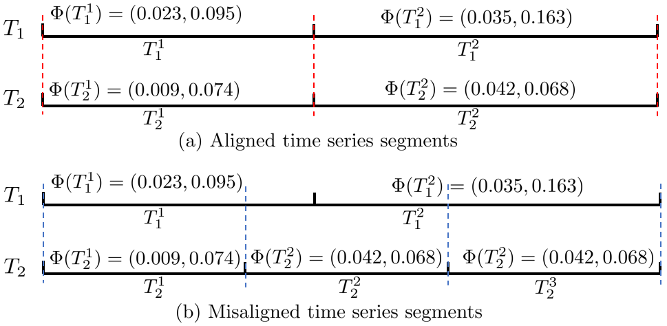
Next, we focus on computing the error measures for derived time series. We first explain the simpler case where each time series is a single segment. Table 8 shows the formulas for computing error measures for derived time series in this case. For the general scenario where multiple segments are involved in each input time series in the expression, there are two cases depending on whether the segments are aligned or not: If the $i$ -th segment in $T_{1}$ has the same domain with the $i$ -th segment in $T_{2}$ for all $i$ , then $T_{1}$ and $T_{2}$ are aligned, otherwise, they are misaligned.

In the following, we will show how to compute the most challenging error guarantee $\hat{\varepsilon}_{Sum(T_{1}\times T_{2})}$ in both aligned and misaligned cases in Section 4.1 and Section 4.2 respectively. The computation of error guarantees of other expressions (i.e., Constant( $\upsilon,a,b$ ), Shift( $\bm{T},k$ ), $\bm{T_{1}+T_{2}}$ and $\bm{T_{1}-T_{2}}$ ) is presented in Appendix C.

4.1. Error Guarantee on Aligned Segments

Notations. Given a time series $\bm{T}=(\bm{T}[a],...,\bm{T}[b])$ and the estimation function $f^{*}_{T}$ of $T$ , $\bm{\varepsilon}_{T}=\bm{T}-f^{*}_{T}=(\bm{T}[a]-f^{*}_{T}(a),...,\bm{T}[b]-f^{*}_{T}(b))$ is the vector of errors produced by the estimation function. In the following, $\bm{T}$ , $f^{*}_{T}$ and $\bm{\varepsilon}$ are all regarded as vectors. $\langle f_{1},f_{2}\rangle=\sum_{i=a}^{b}f_{1}(i)f_{2}(i)$ is the inner product of $f_{1}$ and $f_{2}$ . $V|_{[a,b]}$ is a restriction operation, which restricts a vector $V$ to the domain [a,b]. Recall a time series segment is a subsequence of a time series. Thus, a segment is the restriction of a time series $\bm{T}$ from a bigger domain $[a,b]$ into a smaller domain $[a^{\prime},b^{\prime}]\subseteq[a,b]$ , denoted as $\bm{T}|_{[a^{\prime},b^{\prime}]}$ . Figure 4(b) visualizes the restriction operator. For example, consider a time series $\bm{T}=(1,4,[1.2,1.3,1.3,1.2])$ , then $\bm{T}|_{[2,3]}=(2,3,[1.3,1.3])$ is a restriction of $\bm{T}$ . Note that $\bm{T}|_{[a^{\prime},b^{\prime}]}[i]=T[i]$ for all $i\in[a^{\prime},b^{\prime}]$ .

Given two compressed time series representation $L_{T_{1}}=(\tilde{T_{1}^{1}},...,\tilde{T_{1}^{k}})$ and $L_{T_{1}}=(\tilde{T_{2}^{1}},...,\tilde{T_{2}^{k}})$ for the aligned time series $T_{1}=(T_{1}^{1},...,T_{1}^{k})$ and $T_{2}=(T_{2}^{i},...,T_{2}^{k})$ where $T_{1}^{i}=T_{1}|_{[a_{i},b_{i}]}$ and $T_{2}^{i}=T_{2}|_{[a_{i},b_{i}]}$ . Notice $T_{1}^{i}$ and $T_{2}^{i}$ have the same domain, i.e., $[a_{i},b_{i}]$ , for all $i\in[1,k]$ . For any estimation function family, the error guarantee of Sum( $\bm{T_{1}\times T_{2}}$ ) on aligned time series is:

(2)

\displaystyle\varepsilon\leq\sum_{i=1}^{k}\Big(\|\varepsilon_{T_{1}^{i}}\|_{2}\|\varepsilon_{T_{2}^{i}}\|_{2}+\|\varepsilon_{T_{1}^{i}}\|_{2}\|f_{T_{2}^{i}}\|_{2}+\|f_{T_{1}^{i}}\|_{2}\|\varepsilon_{T_{2}^{i}}\|_{2}\Big)

The details are shown in Appendix D.

Example 0.

Consider the two aligned time series in Figure 6(a). Both $T_{1}$ and $T_{2}$ are partitioned into two segments in this case, i.e., ( $T_{1}^{1},T_{1}^{2}$ ) and ( $T_{2}^{1},T_{2}^{2}$ ). Plato stores the error measures $\Phi(T_{i}^{j})$ for each segment $T_{i}^{j}$ . For instance, $\Phi(T_{1}^{1})=(\|\varepsilon_{T_{1}^{1}}\|_{2},\|f_{T_{1}^{1}}\|_{2},\gamma_{T_{1}^{1}})=(0.023,0.95,0)$ . Then the error guarantee of Sum( $\bm{T_{1}\times T_{2}}$ ) on $T_{1}$ and $T_{2}$ is computed as $(\|\varepsilon_{T_{1}^{1}}\|_{2}\|\varepsilon_{T_{2}^{1}}\|_{2}+\|\varepsilon_{T_{1}^{1}}\|_{2}\|f_{T_{2}^{1}}\|_{2}+\|f_{T_{1}^{1}}\|_{2}\|\varepsilon_{T_{2}^{1}}\|_{2})+(\|\varepsilon_{T_{1}^{2}}\|_{2}\|\varepsilon_{T_{2}^{2}}\|_{2}+\|\varepsilon_{T_{1}^{2}}\|_{2}\|f_{T_{2}^{2}}\|_{2}+\|f_{T_{1}^{2}}\|_{2}\|\varepsilon_{T_{2}^{2}}\|_{2})=(0.023\times 0.009+0.023\times 0.074+0.095\times 0.009)+(0.035\times 0.042+0.035\times 0.068+0.163\times 0.042)=0.01346$ .

4.1.1. Orthogonal projection optimization

If the estimation function family forms a vector space (VS), ¹⁰¹⁰ 10 A vector space is a set that is closed under finite vector addition and scalar multiplication. http://mathworld.wolfram.com/VectorSpace.html. then we can apply the orthogonal projection property in VS to significantly reduce the error guarantee of $sum(T_{1}\times T_{2})$ from Formula 2 to Formula 3.

	$\displaystyle\varepsilon$	$\displaystyle=\Big\|\sum_{i=1}^{k}\Big(\underbrace{\langle\bm{\varepsilon}_{T_{1}^{i}},f^{}_{T_{2}^{i}}\rangle}_{=0~in~VS}+\underbrace{\langle\bm{\varepsilon}_{T_{2}^{i}},f^{}_{T_{1}^{i}}\rangle}_{=0~in~VS}+\langle\bm{\varepsilon}_{T_{1}^{i}},\bm{\varepsilon}_{T_{2}^{i}}\rangle\Big)\Big\|$
(3)			$\displaystyle\leq\sum_{i=1}^{k}\Big(\\|\varepsilon_{T_{1}^{i}}\\|_{2}\\|\varepsilon_{T_{2}^{i}}\\|_{2}\Big)$

Example 0.

Consider the two aligned time series in Figure 6(a) again. The estimation function family is polynomial function family, it is VS. Based on Formula 3, the error guarantee for Sum( $\bm{T_{1}\times T_{2}}$ ) is $\|\varepsilon_{T_{1}^{1}}\|_{2}\times\|\varepsilon_{T_{2}^{1}}\|_{2}$ + $\|\varepsilon_{T_{1}^{2}}\|_{2}\times\|\varepsilon_{T_{2}^{2}}\|_{2}$ = $0.023\times 0.009+0.035\times 0.042=0.001677$ . This error guarantee is about $8\times$ smaller than that in Example 1 (i.e., $0.01346$ ), where we did not take into account that the function family is VS.

Orthogonal projection property. Example 2 indicates the power of the orthogonal projection optimization. Lemma 3 is a proof of Formula 3.

Lemma 0.

(Orthogonal Projection Property) Let $\mathds{F}$ be a function family forms a vector space VS and $f^{*}_{T}\in\mathds{F}$ be the estimation function of time series $T$ . Then $f^{*}_{T}$ is the orthogonal projection of $\mathbf{T}$ onto $\mathds{F}$ (Nelson, 1973).

Lemma 3 implies that $\bm{\varepsilon}_{T}$ is orthogonal to any function $f_{T}\in\mathds{F}$ , which means $\langle\bm{\varepsilon_{T}},\bm{f_{T}}\rangle=0$ . Therefore, given any two aligned segments $T_{1}^{i}$ and $T_{2}^{i}$ , as both $f_{T_{1}^{i}}^{*}$ and $f_{T_{2}^{i}}^{*}$ are in VS, thus $\langle\bm{\varepsilon}_{T_{1}^{i}},f^{*}_{T_{2}^{i}}\rangle=0$ and $\langle\bm{\varepsilon}_{T_{2}^{i}},f^{*}_{T_{1}^{i}}\rangle=0$ .

For visualization purposes, consider a time series with three data points $T=(1,3,[3.0,4.8,5.4])$ and let $\mathds{F}$ be the 1-degree polynomial function family (i.e., 2-dimensional). The estimation function that minimizes the error to the original data is $f^{*}_{T}=1.2\times i+2$ (Figure 8(a)). As shown in Figure 8(b), $f^{*}_{T}$ is the orthogonal projection of $\bm{T}$ onto $\mathds{F}$ . The error vector is $\bm{\varepsilon}_{T}=(-0.2,0.4,-0.2)$ . Based on Lemma 3, for any candidate estimation function $f=\alpha\times i+\beta$ $(\alpha,\beta\in R)$ , we have $\langle\bm{\varepsilon_{T}},\bm{f}\rangle=0.8\alpha-0.8\alpha+0.4\beta-0.4\beta=0$ .

Elimination of $\gamma_{T}$ . We can get an extra benefit from the orthogonal projection property in saving space, i.e., the error measure $\gamma_{T}$ can be avoided as it is guaranteed to be $0$ . This is because $\gamma_{T}=\langle T-f^{*}_{T},1\rangle$ and $1$ is a constant function in the function family in VS. According to Lemma 3, we know $\langle T-f^{*}_{T},1\rangle=0$ . Therefore, we have $\gamma_{T}=0$ .

Amplitude-independent (AI). The orthogonal projection optimization can significantly reduce the error guarantees. It allows the error guarantees to get rid of the amplitudes of the original time series values (referring to $\|f_{T}\|_{2}$ ) by only consider the reconstruction error (referring to $\|\varepsilon_{T}\|_{2}$ ) of each time series. The error guarantees provided by Plato in VS are called amplitude-independent (AI) error guarantees.

4.2. Error Guarantee on Misaligned Segments

Given two compressed time series representation $L_{T_{1}}=(\tilde{T_{1}^{1}},...,\tilde{T_{1}^{k_{1}}})$ and $L_{T_{1}}=(\tilde{T_{2}^{1}},...,\tilde{T_{2}^{k_{2}}})$ for the misaligned time series $T_{1}=(T_{1}^{1},...,T_{1}^{k_{1}})$ and $T_{2}=(T_{2}^{1},...,T_{2}^{k_{2}})$ where the domains of $T_{1}^{i}$ and $T_{2}^{i}$ are $[a_{i}^{1},b_{i}^{1}]$ and $[a_{i}^{2},b_{i}^{2}]$ respectively. The major challenge in the misaligned case is that for a domain $[a_{1}^{i},b_{1}^{i}]$ , the error measures of the segment $T_{1}|_{[a_{1}^{i},b_{1}^{i}]}$ are precomputed, however, the error measures of the segment $T_{2}|_{[a_{1}^{i},b_{1}^{i}]}$ may be unknown as $T_{2}|_{[a_{1}^{i},b_{1}^{i}]}$ in general is not one of the segments $T_{2}^{1},...,T_{2}^{k_{2}}$ .

Let $\Pi_{T,[a,b]}$ be the set of segments in $T$ covering the domain $[a,b]$ . For example, consider the two misaligned time series $T_{1}$ and $T_{2}$ in Figure 6(b), $\Pi_{T_{2},[a_{1}^{1},b_{1}^{1}]}$ = $\{T_{2}^{1},T_{2}^{2}\}$ as the segments $T_{2}^{1}$ and $T_{2}^{2}$ in $T_{2}$ cover the domain $[a_{1}^{1},b_{1}^{1}]$ . ¹¹¹¹ 11 If time series $T_{1}$ and $T_{2}$ are aligned, then $\Pi_{T_{2},[a_{1}^{i},b_{1}^{i}]}$ always returns one single segment. If any kinds of function families are allowed, i.e., in ANY, the error guarantee $\hat{\varepsilon}$ of Sum( $\bm{T_{1}\times T_{2}}$ ) on misaligned time series is:

Formula 4 is a stepping stone towards producing the final formula as the computation of $|\langle\bm{\varepsilon_{T_{1}}},\bm{\varepsilon_{T_{2}}}\rangle|$ (Formula 4 $\textcircled{2}$ ) has not been given yet. It will be discussed in Section 4.2.1. Section 4.2.2 discusses how to apply the orthogonal property optimization to improve Formula 4 $\textcircled{1}$ .

4.2.1. Segment combination selection

To compute $|\langle\bm{\varepsilon_{T_{1}}},\bm{\varepsilon_{T_{2}}}\rangle|$ , one straightforward method (called IS) is to use the domains of segments in $T_{1}$ and $T_{2}$ independently, then choose the one with minimal value. Let’s first see how to compute $|\langle\bm{\varepsilon_{T_{1}}},\bm{\varepsilon_{T_{2}}}\rangle|$ with the domains of segments in $T_{1}$ .

	$\displaystyle\|\langle\bm{\varepsilon_{T_{1}}},\bm{\varepsilon_{T_{2}}}\rangle\|$	$\displaystyle\leq\sum_{i=1}^{k_{1}}\big\|\langle\bm{\varepsilon_{T_{1}\|_{[a_{1}^{i},b_{1}^{i}]}}},\bm{\varepsilon_{T_{2}\|_{[a_{1}^{i},b_{1}^{i}]}}}\rangle\big\|=\sum_{i=1}^{k_{1}}\big\|\langle\bm{\varepsilon_{T_{1}^{i}}},\bm{\varepsilon_{T_{2}\|_{[a_{1}^{i},b_{1}^{i}]}}}\rangle\big\|$
		$\displaystyle\leq\sum_{i=1}^{k_{1}}\big(\\|\varepsilon_{T_{1}^{i}}\\|_{2}(\sum_{j\in\Pi_{T_{2},[a_{1}^{i},b_{1}^{i}]}}\\|\varepsilon_{T_{2}^{j}}\\|_{2}^{2})^{\frac{1}{2}}\big)$

In the last step of the above Formula, $T_{2}|_{[a_{1}^{i},b_{1}^{i}]}$ is not a segment that Plato precomputed in $T_{2}$ . Thus, we need to use all the segments in $T_{2}$ covering $[a_{1}^{i},b_{1}^{i}]$ , i.e., $\Pi_{T_{2},[a_{1}^{i},b_{1}^{i}]}$ . Similarly, we can compute $|\langle\bm{\varepsilon_{T_{1}}},\bm{\varepsilon_{T_{2}}}\rangle|$ according to the domains of segments in $T_{2}$ . Finally, IS chooses the minimal one between them. However, IS does not produce tight guarantees, Plato does not use it. Next, we show the tight computation called OS, which is used by Plato.

Optimal strategy (OS) OS (Algorithm 1) first computes an error distribution array $E_{T_{1}}$ (resp. $E_{T_{2}}$ ) for $T_{1}$ (resp. $T_{2}$ ) (line 2) according to the domains of the segments as follows:

	$\displaystyle E_{T_{1}}=\Big\{\\|\varepsilon_{T_{1}^{i}}\\|_{2}\times\Big(\sum_{j\in\Pi_{T_{2},[a_{1}^{i},b_{1}^{i}]}}\\|\varepsilon_{T_{2}^{i}}\\|_{2}^{2}\Big)^{\frac{1}{2}}\Big\|1\leq i\leq k_{1}\Big\}$
	$\displaystyle E_{T_{2}}=\Big\{\\|\varepsilon_{T_{2}^{i}}\\|_{2}\times\Big(\sum_{j\in\Pi_{T_{1},[a_{2}^{i},b_{2}^{i}]}}\\|\varepsilon_{T_{1}^{i}}\\|_{2}^{2}\Big)^{\frac{1}{2}}\Big\|1\leq i\leq k_{2}\Big\}$

Then OS increases $\varepsilon_{1}$ (resp. $\varepsilon_{2}$ ) by adding the values from $E_{T_{1}}$ (resp. $E_{T_{2}}$ ) (lines 4-7) and checks whether the current domain achieves the minimal errors (lines 8-17). If yes, OS adds the current domain (either $[start,b_{1}^{i_{1}}]$ or $[start,b_{2}^{i_{2}}]$ ) to the final segment combination list. After that, OS starts from a new domain and repeats the previous steps until all the segments are processed. The time complexity of OS is $O(k_{1}+k_{2})$ .

Let $OPT(L_{T_{1}},L_{T_{2}})$ be the segment combination returned by OS. Then $|\langle\bm{\varepsilon_{T_{1}}},\bm{\varepsilon_{T_{2}}}\rangle|$ is computed as follows:

		$\displaystyle\|\langle\bm{\varepsilon_{T_{1}}},\bm{\varepsilon_{T_{2}}}\rangle\|\leq\sum_{[a,b]\in OPT(L_{T_{1}},L_{T_{2}})}\Big\|\langle\bm{\varepsilon_{T_{1}}}\|_{[a,b]},\bm{\varepsilon_{T_{2}}}\|_{[a,b]}\rangle\Big\|$
		$\displaystyle\leq\sum_{[a,b]\in OPT(L_{T_{1}},L_{T_{2}})}\Big(\Big(\sum_{i\in\Pi_{T_{1},[a,b]}}\\|\bm{\varepsilon_{T_{1}^{i}}}\\|_{2}^{2}\Big)^{\frac{1}{2}}\Big(\sum_{i\in\Pi_{T_{2},[a,b]}}\\|\bm{\varepsilon_{T_{2}^{i}}}\\|_{2}^{2}\Big)^{\frac{1}{2}}\Big)$

OS provides the optimal segment combination that produces the minimum $|\langle\bm{\varepsilon_{T_{1}}},\bm{\varepsilon_{T_{2}}}\rangle|$ . The tightness proof is presented in Appendix E.

Example 0.

Consider the two misaligned time series in Figure 8. The value of $\|\varepsilon_{T_{i}^{j}}\|_{2}$ for each segment $T_{i}^{j}$ is labeled there. OS produces the segment combination $S=\{[a_{1}^{1},b_{2}^{1}],[b_{2}^{1},b_{2}^{101}]\}$ as visualized by the red lines. Then $|\langle\bm{\varepsilon_{T_{1}}},\bm{\varepsilon_{T_{2}}}\rangle|=(3\times(96\times 1^{2}+2^{2})^{\frac{1}{2}})+(2\times(100\times 1^{2})^{\frac{1}{2}})=3\times 10+2\times 10=50$ . However, IS outputs $|\langle\bm{\varepsilon_{T_{1}}},\bm{\varepsilon_{T_{2}}}\rangle|=min((3\times 96+2\times\sqrt{100+9}),(3\times\sqrt{96+2^{2}}+100\times 2))=\min(308.88,230)=230$ , which is $4.6\times$ larger than the result returned by OS.

Algorithm 1 Optimal segment combination (OS)

Input: Compressed segment representations

L_{T_{1}}

L_{T_{2}}

Output: A segment combination

OPT

\varepsilon_{1}=0

\varepsilon_{2}=0

i_{i}=0

i_{2}=0

start=0

OPT=\emptyset

current

\emptyset

;

2 Compute

E_{T_{1}}

and

E_{T_{2}}

;

3 while $i_{1}<k_{1}$ or $i_{2}<k_{2}$ do

4 if $b_{1}^{i_{1}}\leq b_{2}^{i_{2}}$ then

\varepsilon_{1}+=E_{T_{1}}[i_{1}++]

;

6 else

\varepsilon_{2}+=E_{T_{2}}[i_{2}++]

;

8 if $\varepsilon_{1}\leq\varepsilon_{2}$ AND $b_{1}^{i_{1}}\geq b_{2}^{i_{2}}$ then

current=[start,b_{1}^{i_{1}}]

;

OPT\leftarrow OPT\cup\{current\}

;

start=b_{1}^{i_{1}}+1

;

\varepsilon_{2}\leftarrow\varepsilon_{1}

;

13 if $\varepsilon_{2}\leq\varepsilon_{1}$ AND $b_{2}^{i_{2}}\geq b_{1}^{i_{1}}$ then

current=[start,b_{2}^{i_{2}}]

;

OPT\leftarrow OPT\cup\{current\}

;

start=b_{2}^{i_{2}}+1

;

\varepsilon_{1}\leftarrow\varepsilon_{2}

;

18 Return

OPT

;

4.2.2. Orthogonal projection optimization

In this part, we present how to apply orthogonal property optimization to improve Formula 4 $\textcircled{1}$ . Recall that in the aligned case (if the function family is in VS) we can apply the orthogonal property optimization to guarantee $\langle\varepsilon_{T_{1}^{i}},f^{*}_{T_{2}}|_{[a_{1}^{i},b_{1}^{i}]}\rangle=0$ . This is because $f^{*}_{T_{2}}|_{[a_{1}^{i},b_{1}^{i}]}=f^{*}_{T_{2}^{i}}$ , which is a function in the family. However, in misaligned case $\langle\varepsilon_{T_{1}^{i}},f^{*}_{T_{2}}|_{[a_{1}^{i},b_{1}^{i}]}\rangle$ cannot be guaranteed to be $0$ since $f^{*}_{T_{2}}|_{[a_{1}^{i},b_{1}^{i}]}$ may not be a function in the family. For example, in Figure 8 $T_{2}|_{[a_{2}^{1},b_{2}^{1}]}$ is not a pre-computed segment in $T_{2}$ , it is just a subsegment. The restriction of the estimation function $f^{*}_{T_{2}^{1}}$ to this sub-domain $f^{*}_{T_{2}}|_{[a_{1}^{1},b_{1}^{1}]}$ may not be a function in the family anymore.

To guarantee the restriction of the function from a bigger domain to a smaller domain is still in the same function family, we identify a function family group called linear scalable function family (LSF), which is subset of VS but superset of the polynomial function family.

Linear Scalable Function Family (LSF). Informally, a linear scalable family is a function family such that for any function $f$ in that family and any translation $a-a^{\prime}$ , there is a function $f^{\prime}$ in that family such that $f^{\prime}(x+a-a^{\prime})=f(x)$ for all x in the domain. Definition 5 gives the formal definition.

Definition 0 (Linear scalable family (LSF)).

Let $\mathds{F}$ be a function family defined in domain $[a,b]$ , $\mathds{F}$ is a linear scalable family if for any function $f\in\mathds{F}$ and any range $[a^{\prime},b^{\prime}]\subseteq[a,b]$ , there exists a function $f^{\prime}\in\mathds{F}$ such that Shift $(f|_{[a^{\prime},b^{\prime}]},$ $a-a^{\prime})$ = $f^{\prime}|_{[a,a+b^{\prime}-a^{\prime}]}$ .

Lemma 0.

The polynomial family belongs to the linear scalable family.

The proof of Lemma 6 is shown in Appendix F.

Recall that, in this paper, we study three different function family groups, i.e., ANY, VS, and LSF. Figure 3 shows the relation of the three function family groups and also provides example function families for each group.

In the following, we present how to use the orthogonal projection optimization in the misaligned case to improve Formula 4 $\textcircled{1}$ . Let $\bm{f_{T_{1}}}$ (resp. $\bm{f_{T_{2}}}$ ) be the function created from the concatenation of the individual estimation functions on the segments $T_{1}^{i}$ $(i\in[1,k_{1})$ (resp. $T_{2}^{j}$ $(j\in[1,k_{2}]$ )). That is $\bm{f_{T_{1}}|_{[a_{1}^{i},b_{1}^{i}]}}=f^{*}_{T_{1}^{i}}$ for all $i\in[1,k_{1}]$ and $\bm{f_{T_{2}}|_{[a_{2}^{i},b_{2}^{i}]}}=f^{*}_{T_{2}^{i}}$ for all $i\in[1,k_{2}]$ . Then the Equation 4 $\textcircled{1}$ in the misaligned environment can be reduced as follows. We highlight the parts that would disappear if the segments were aligned.

		$\displaystyle\sum_{i=1}^{k_{1}}\Big(\\|\varepsilon_{T_{1}^{i}}\\|_{2}\times\overbrace{\\|\bm{f_{T_{2}}\|_{[a_{1}^{i},b_{1}^{i}]}-f^{*}_{T_{1}^{i}}}\\|_{2}}^{=0~if~aligned}\Big)$
	$\displaystyle+$	$\displaystyle\sum_{i=1}^{k_{2}}\Big(\\|\varepsilon_{T_{2}^{i}}\\|_{2}\times\overbrace{\\|\bm{f_{T_{1}}\|_{[a_{2}^{i},b_{2}^{i}]}-f^{*}_{T_{2}^{i}}}\\|_{2}}^{=0~if~aligned}\Big)~~~~~~~~(5)$

The proof of the tightness is in Appendix G.

Efficient Computation of the Error Guarantee Notice that both $\|\bm{f_{T_{2}}|_{[a_{1}^{i},b_{1}^{i}]}-f^{*}_{T_{1}^{i}}}\|_{2}$ and $\|\bm{f_{T_{1}}|_{[a_{2}^{i},b_{2}^{i}]}-f^{*}_{T_{2}^{i}}}\|_{2}$ can only be computed during query processing time, since only then the pairs of intersecting but misaligned segments become known. A brute force $O(n)$ method, where $n$ is the size of the domain of the segment, would be to literally create the series of $n$ data points predicted by the estimation functions and then perform the straightforward calculation/aggregation described by the formulas. Of course, such brute force approach would require CPU cycles that are proportional to conventional (non-approximate) query processing. We show that these formulas can be computed in $O(dim(\mathds{F})^{3})$ where $dim(\mathds{F})$ is the dimension of the estimation function family. Obviously, the dimension is much smaller than the number of data points in a segment - that is why we employ compression in the first place. For example, for a $1$ -degree polynomial function family, $dim(\mathds{F})=2$ . The key intuition is to store the estimation function’s coefficients in an orthonormal basis. The distance between two functions can be efficiently computed using the $dim(\mathds{F})$ coefficients (in the orthonormal basis). Importantly, the orthonormal basis also allows us to compute the coefficients of the restriction of an estimation function in $O(dim(\mathds{F})^{3})$ . The detailed algorithms and proofs complexity appear in the Appendix H.

Elimination of $\|f_{T}\|_{2}$ . If $T$ is compressed by a function in LSF ¹²¹² 12 And we know that it many only be combined with other segments compressed by a function in LSF., then $\|f_{T}\|_{2}$ can be safely eliminated. This is because the error guarantees provided by LSF can get rid of $\|f_{T}\|_{2}$ while those given by ANY or VS rely on $\|f_{T}\|_{2}$ .

	avg $\#$ of data points	$\#$ of	resolution
	in each time series	time series	resolution
HF	$126,059,817$	15	millisecond
HI	$2,676,311$	14	second
HB	$1,669,835$	16	minute
HA	$1,587,258$	11	minute

Table 5. Data Characteristics

	$\#$ of coefficients	$\#$ of error measures
Polynomial	$2$	$1$
Gaussian	$4$	$3$

Table 6. Number of coefficients and error measures

5. Experiments

5.1. Environment and Setting

All experiments were conducted on a computer with a $4^{th}$ Intel $i7$ - $4770$ processor ( $3.6$ GHz), $16$ GB RAM, running Ubuntu $14.04.1$ . The algorithms were implemented in $C++$ and were compiled with $g$ ++ $4.8.4$ .

Dataset. We evaluated all the error guarantee methods on four real-life datasets: Historical Forex Data (HF), Historical IoT Data (HI), Historical Bitcoin Exchanges Data (HB), and Historical Air Quality Data (HA). Table 6 summarizes the data characteristics. The detailed description of each dataset is presented in Appendix I.

Segmentation algorithms. We adopt the fixed-length segmentation (FL) and the sliding window algorithm (SW). The segments produced by the FL have equal lengths, and will be utilized in our aligned experiments, while the segments created by the SW have variable lengths and are used in our misaligned experiments.

Estimation function families. Following the prior work lessons (Keogh, 1997; Pan et al., 2017), we choose the 1-degree polynomial function family ( $\{ax+b|a,b\in R\}$ ) and the Gaussian function family ( $\{a\exp\Big(\frac{-(x-b)^{2}}{2c^{2}}\Big)+d|a,b,c,d\in R\}$ ) as representatives to compress the time series. Notice that the Gaussian function family is in ANY, while the polynomial function family is in LSF (also in VS). Table 6 summarizes the number of coefficients and error measures stored for each segment compressed by the corresponding estimation functions.

Queries We evaluate the correlation TSA over all the time series pairs in each dataset. The corresponding SQL queries are shown in Appendix I. All the error guarantees and true errors reported in the following are the average values (including the standard variances) across all correlations in a dataset.

5.2. Experimental Results

We evaluate the error guarantees for TSAs over aligned, fixed-length time series segmentations and misaligned, variable-length time series segmentations. In order to provide a fair comparison, we fix the space cost for both cases, i.e., they have the same compression ratios.

Error Guarantees Quality Figure 9 reports the absolute true errors and the error guarantees of the correlation TSAs in the aligned/fixed-length (FL) and misaligned/variable-length (SW) cases using the polynomial function family. Since the TSAs are correlations, the approximate results may range between 1 (perfect correlation) and -1 (perfect reverse correlation), with 0 meaning no correlation at all.

Under the same compression ratio ¹³¹³ 13 Compression ratio is the size of the original data over the size of the compressed data. the variable-length error guarantees are much smaller than the fixed-length error guarantees. In Figure 9, the misaligned Error-Guarantee (SW) is $10\times\sim 20\times$ smaller than the aligned Error-Guarantee (FL) on the average (ranging the compression ratio from $10,000$ to $100$ ). This is mainly because, as it has already been known, variable-length allows for much better estimation. Indeed, notice the misaligned true errors are also much smaller than the aligned true errors. For example, In Figure 9, True-Error(SW) is $6\times\sim 11\times$ smaller than True-Error(FL) on the average.

Importantly, the error guarantees are close to the true errors, especially for the misaligned error guarantees, which matter most practically. In particular, Error-Guarantee(SW) is only $1.08\times\sim 1.11\times$ larger than the True-Error(SW) in HF and HI respectively (on the average). Furthermore, they are very small in absolute terms. This indicates the high quality and practicality of AI (Amplitude-independent) error guarantees.

Run time performance Figure 10 reports the total running time of the correlation TSAs over (i) the original time series (Original), (ii) the time series segmented into a fixed length, aligned segments (Plato-FL) and (iii) time series segmented into misaligned, variable-length segments by SW (Plato-SW). The estimation function family is the polynomial family. The x-axis is the compression ratio (from $10000$ to $100$ ).

Both Plato-FL and Plato-SW outperform vastly the Original in all the datasets. For example, when the compression ratio is $1000$ , Plato-FL and Plato-SW are about three orders of magnitude faster than Original.

Plato-SW is about $1.8\times$ slower than Plato-FL due to the intricacy of the segment combination selection algorithm. However, a mere 80% penalty is a minor price to pay for the orders-of-magnitude superior error guarantees delivered by misaligned/variable-length segmentations.

Comparison with sampling In this part, we compare (i) the space cost and (ii) the runtime performance of Plato with the sampling methods when providing similar error guarantees. We use a uniform random sampling scheme with a global seed in order to create a samples database. We also assume knowledge of minimums and maximums. That is, let $X_{1},...,X_{n}$ be the random variables such that $d_{min}\leq X_{i}\leq d_{max}$ for all $i$ where $X_{i}=d^{T_{1}}_{i}\times d^{T_{2}}_{i}$ , $d_{min}=\min\{d^{T_{1}}_{i}\}\times\min\{d^{T_{2}}_{i}\}$ , and $d_{max}=\max\{d^{T_{1}}_{i}\}\times\max\{d^{T_{2}}_{i}\}$ . Let $R=\sum_{i=1}^{n}X_{i}$ and $\varepsilon$ be the error guarantee. Using the Chernoff bounds (Hagerup and Rüb, 1990), we can obtain the minimal sample size needed in order to achieve the desired error guarantee with certain confidence.

Figure 12 reports the sizes (as percentage to the original data size) of sampled data points in order to provide similar error guarantees with the Plato-FL (the error guarantee of TSAs over aligned, fixed-length time series produced by FL) and Plato-SW (the error guarantee of TSAs over misaligned time series produced by SW) with $1000$ compression ratio in HF respectively. Figure 12 shows the corresponding runtime cost. To achieve similar error guarantees, sampling needs more space and more time than Plato. We define “similar" to mean 90%, or 95% or 99% confidence - in contrast to Plato’s deterministic, 100% confidence guarantees.

5.2.1. Effects of Individual Factors

In this part, we study the effects of (i) compression ratios, (ii) estimation function families, (iii) orthogonal optimizations, and (iv) segment combination selection strategies.

Compression ratios In order to isolate the effect of the compression ratios, ¹⁴¹⁴ 14 Compression ratio is the size of the original data over the size of the compressed data. we fix the estimation function family to be polynomials and fix the segment list building algorithm to be SW. In Figure 14, we change the compression ratios from $10,000$ to $100$ by controlling the error threshold values and report the corresponding true errors (True-Error(SW)) and the error guarantees (Error-Guarantee(SW)).

Naturally, higher compression ratios lead to smaller true errors and error guarantees. For example, in Figure 14(a), the true error and error guarantee with $100$ compression ratio are $13.32\times$ and $15.58\times$ smaller than those with $10,000$ compression ratio on the average. Importantly, the error guarantees provided by Plato are close to the true error in all the datasets and are generally small in absolute terms (with the relative exception of $10,000$ compression on HF). Again, this indicates the high quality of the error guarantees provided by Plato.

Estimation function families In order to isolate the effect of the estimation function families, we fix the segment list building algorithm to be SW and fix the compression ratio to $1000$ . Figure 14 presents the true errors and the error guarantees for TSAs over time series compressed by polynomial functions (True-Error(Poly), Error-Guarantee(Poly)) and Gaussian functions (True-Error(Gau), Error-Guarantee(Gau)) respectively.

The error guarantees with estimation functions from LSF (polynomials) are significantly smaller than those with estimation functions in ANY (Gaussians). In Figure 14(a), Error-Guarantee(Poly) (in LSF and VS) is about $10\times$ smaller than Error-Guarantee(Gau) (in ANY) on the average and in Figure 14(b), Error-Guarantee(Poly) (in LSF and VS) is about $160\times$ smaller than Error-Guarantee(Gau) (in ANY) on the average. Notice that the error guarantees provided by Plato-Poly is AI, while those of Plato-Gau are not. So the results show that AI error guarantees are practical while non-AI error guarantees are not. Interestingly, True-Error(Gau) is smaller than True-Error(Poly) in the HF dataset, which indicates that Gaussian functions model HF data better than the polynomial functions - not surprising given the more random movements of financial data. The guarantees produced by the polynomials are far better thanks to AI.

Effect of Orthogonal Optimization and LSF To measure the effect on error guarantees of the orthogonal optimization (and its extension to misaligned segmentations, enabled by LSF) we fix the estimation function family to the polynomials, which are LSF and, trivially, are also in ANY. We use both the general error guarantees of ANY (Error-Guarantee(ANY)) and the specialized error guarantees of LSF (Error-Guarantee(LSF)) for TSAs over misaligned segments compressed by polynomial functions (using variable-length segmentations with the SW algorithm). We fix the compression ratio to $1000$ . As shown in Figure 16, the error guarantee for LSF certifies that the true result is just within $\pm 0.0137$ in HF and within $\pm 0.0052$ in HI.

Segment combination selection strategies To isolate the quality effect of employing the optimal segment combination selection strategy (OS) we compare it with IS strategy (the straightforwad method mentioned in Section 4.2.1) on a case of variable-length compression with an LSF function family (polynomials). Figure 16 shows that Plato-OS is about $5\times$ smaller than Plato-MS on the average. In addition, the running time of Plato-IS and Plato-OS are close. For example, the running time of Plato-IS and Plato-OS are $0.536$ and $0.548$ seconds in HF respectively.

6. Related Work

Approximate query processing (AQP) and data compression have been widely studied. whose most relevant aspects are summarized next.

AQP with probabilistic error guarantees. Approximate query processing using sampling (Chaudhuri et al., 2007; Sidirourgos et al., 2011; Pansare et al., 2011; Agarwal et al., 2013) computes approximate answers by appropriately evaluating the queries on small samples of the data, e.g., STRAT (Chaudhuri et al., 2007), SciBORQ (Sidirourgos et al., 2011), and BlinkDB (Agarwal et al., 2013). Such approaches typically leverage statistical inequalities and the central limit theorem to compute the confidence interval (or variance) of the computed approximate answer. As a result, their error guarantees are probabilistic - as opposed to this work’s deterministic (100% confidence) ones. Note however that, unlike sampling, our compression-based techniques are tuned for time series and continuous data.

AQP with deterministic error guarantees. Approximately answering queries while providing deterministic error guarantees has been successfully applied in many applications (Cormode et al., 2005; Greenwald and Khanna, 2001; Manku et al., 1998; Potti and Patel, 2015; Lazaridis and Mehrotra, 2001; Poosala et al., 1996). However, existing work in the area has focused on simple aggregation queries that involve only a single time series (or table) and aggregates such as SUM, COUNT, MIN, MAX and AVG. Our work extends the prior work, as it addresses analytics over multiple compressed time series such as correlation, cross-correlation. In addition, this work is the first one to categorize compression function families based on their suitability for error guarantees.

Data summarizations and compressions The database community has mostly focused on creating summarizations (also referred to as synopses or sketches) that can be used to answer specific queries. These include among others histograms (Piatetsky-Shapiro and Connell, 1984; Ioannidis and Poosala, 1995; Wang and Sevcik, 2008; Reiss et al., 2006) (e.g., EquiWidth and EquiDepth histograms (Piatetsky-Shapiro and Connell, 1984), V-Optimal histograms (Ioannidis and Poosala, 1995), and Hierarchical Model Fitting (HMF) histograms (Wang and Sevcik, 2008)), used among other for cardinality estimation (Ioannidis and Poosala, 1995) and selectivity estimation (Poosala et al., 1996). The signal processing community produced a variety of methods that can be used to compress time series data and thus are more relevant to the present work, as they provide the underlying compressions. These include among others the Piecewise Aggregate Approximation (PAA) (Keogh et al., 2001a), and the Piecewise Linear Representation (PLR) (Keogh, 1997). Plato is orthogonal to those data summarization and compression techniques.

7. Summary and Future Direction

This work indicates that deterministic error guarantees are feasible and practical, given the appropriate combination of error measures and estimation function family. Future work may develop such combinations for other important families also. Note that the tightness results of this paper do not preclude the future development of practical and theoretically-sound deterministic error guarantees for families are currently outside the LSF (or outside the VS in the case of aligned series). Researchers may come up with other interesting properties of function families outside LSF (or VS) and deliver good error guarantees, based on such properties.

References

Agarwal et al. (2013) Sameer Agarwal, Barzan Mozafari, Aurojit Panda, Henry Milner, Samuel Madden, and Ion Stoica. 2013. BlinkDB: queries with bounded errors and bounded response times on very large data. In EuroSys. 29–42.
Aghabozorgi et al. (2015) Saeed Reza Aghabozorgi, Ali Seyed Shirkhorshidi, and Ying Wah Teh. 2015. Time-series clustering - A decade review. Inf. Syst. 53 (2015), 16–38.
Chan and Fu (1999) Kin-pong Chan and Ada Wai-Chee Fu. 1999. Efficient Time Series Matching by Wavelets. In ICDE. 126–133.
Chaudhuri et al. (2007) Surajit Chaudhuri, Gautam Das, and Vivek Narasayya. 2007. Optimized stratified sampling for approximate query processing. TODS 32, 2 (2007), 9.
Chaudhuri et al. (2017) Surajit Chaudhuri, Bolin Ding, and Srikanth Kandula. 2017. Approximate query processing: no silver bullet. In Sigmod. ACM, 511–519.
Chen and Ng (2004) Lei Chen and Raymond T. Ng. 2004. On The Marriage of Lp-norms and Edit Distance. In VLDB. 792–803.
Cheney and Kincaid (2009) Ward Cheney and David Kincaid. 2009. Linear algebra: Theory and applications. The Australian Mathematical Society 110 (2009).
Choi (2012) ByoungSeon Choi. 2012. ARMA model identification. Springer Science & Business Media.
Cormode et al. (2005) Graham Cormode, Flip Korn, S. Muthukrishnan, and Divesh Srivastava. 2005. Effective Computation of Biased Quantiles over Data Streams. In ICDE. 20–31.
Denison et al. (1998) DGT Denison, BK Mallick, and AFM Smith. 1998. Automatic Bayesian curve fitting. Journal of the Royal Statistical Society: Series B (Statistical Methodology) 60, 2 (1998), 333–350.
Eisenberg and Melton (2002) Andrew Eisenberg and Jim Melton. 2002. SQL/XML is making good progress. ACM Sigmod Record 31, 2 (2002), 101–108.
Faloutsos et al. (1994) Christos Faloutsos, M. Ranganathan, and Yannis Manolopoulos. 1994. Fast Subsequence Matching in Time-Series Databases. In SIGMOD. 419–429.
Galakatos et al. (2017) Alex Galakatos, Andrew Crotty, Emanuel Zgraggen, Carsten Binnig, and Tim Kraska. 2017. Revisiting reuse for approximate query processing. Proceedings of the VLDB Endowment 10, 10 (2017), 1142–1153.
Greenwald and Khanna (2001) Michael Greenwald and Sanjeev Khanna. 2001. Space-Efficient Online Computation of Quantile Summaries. In SIGMOD. 58–66.
Hagerup and Rüb (1990) Torben Hagerup and Christine Rüb. 1990. A guided tour of Chernoff bounds. Information processing letters 33, 6 (1990), 305–308.
Hoffmann (1989) Walter Hoffmann. 1989. Iterative algorithms for Gram-Schmidt orthogonalization. Computing 41, 4 (1989), 335–348.
Ioannidis and Poosala (1995) Yannis E. Ioannidis and Viswanath Poosala. 1995. Balancing Histogram Optimality and Practicality for Query Result Size Estimation. In SIGMOD. 233–244.
Keogh (1997) Eamonn Keogh. 1997. Fast similarity search in the presence of longitudinal scaling in time series databases. In ICTAI. 578–584.
Keogh et al. (2001b) Eamonn Keogh, Selina Chu, David Hart, and Michael Pazzani. 2001b. An online algorithm for segmenting time series. In ICDM. 289–296.
Keogh et al. (2004) Eamonn Keogh, Selina Chu, David Hart, and Michael Pazzani. 2004. Segmenting time series: A survey and novel approach. In Data mining in time series databases. World Scientific, 1–21.
Keogh et al. (2001a) Eamonn J. Keogh, Kaushik Chakrabarti, Michael J. Pazzani, and Sharad Mehrotra. 2001a. Dimensionality Reduction for Fast Similarity Search in Large Time Series Databases. KAIS 3, 3 (2001), 263–286.
Keogh and Pazzani (1998) Eamonn J. Keogh and Michael J. Pazzani. 1998. An Enhanced Representation of Time Series Which Allows Fast and Accurate Classification, Clustering and Relevance Feedback. In KDD. 239–243.
Keogh and Pazzani (1999) Eamonn J Keogh and Michael J Pazzani. 1999. Relevance feedback retrieval of time series data. In SIGIR. 183–190.
Kim (2003) Kyoung-jae Kim. 2003. Financial time series forecasting using support vector machines. Neurocomputing 55, 1-2 (2003), 307–319.
Koski et al. (1995) Antti Koski, Martti Juhola, and Merik Meriste. 1995. Syntactic recognition of ECG signals by attributed finite automata. Pattern Recognition 28, 12 (1995), 1927–1940.
Kovács et al. (2002) Geza Kovács, Shay Zucker, and Tsevi Mazeh. 2002. A box-fitting algorithm in the search for periodic transits. Astronomy & Astrophysics 391, 1 (2002), 369–377.
Kumar et al. (2015) Arun Kumar, Robert McCann, Jeffrey F. Naughton, and Jignesh M. Patel. 2015. Model Selection Management Systems: The Next Frontier of Advanced Analytics. SIGMOD Record 44, 4 (2015), 17–22.
Lazaridis and Mehrotra (2001) Iosif Lazaridis and Sharad Mehrotra. 2001. Progressive Approximate Aggregate Queries with a Multi-Resolution Tree Structure. In SIGMOD. 401–412.
Lazaridis and Mehrotra (2003) Iosif Lazaridis and Sharad Mehrotra. 2003. Capturing Sensor-Generated Time Series with Quality Guarantees. In Proceedings of the 19th International Conference on Data Engineering, March 5-8, 2003, Bangalore, India. 429–440.
Li et al. (1998) Chung-Sheng Li, Philip S. Yu, and Vittorio Castelli. 1998. MALM: A Framework for Mining Sequence Database at Multiple Abstraction Levels. In CIKM. 267–272.
Manku et al. (1998) Gurmeet Singh Manku, Sridhar Rajagopalan, and Bruce G. Lindsay. 1998. Approximate Medians and other Quantiles in One Pass and with Limited Memory. In SIGMOD. 426–435.
Mei and Moura (2017) Jonathan Mei and José M. F. Moura. 2017. Signal Processing on Graphs: Causal Modeling of Unstructured Data. IEEE Trans. Signal Processing 65, 8 (2017), 2077–2092.
Morse and Patel (2007) Michael D. Morse and Jignesh M. Patel. 2007. An efficient and accurate method for evaluating time series similarity. In SIGMOD. 569–580.
Nelson (1973) Edward Nelson. 1973. Probability theory and Euclidean field theory. In Constructive quantum field theory. Springer, 94–124.
Pan et al. (2017) Zhuokun Pan, Yueming Hu, and Bin Cao. 2017. Construction of smooth daily remote sensing time series data: a higher spatiotemporal resolution perspective. Open Geospatial Data, Software and Standards 2, 1 (2017), 25.
Pansare et al. (2011) Niketan Pansare, Vinayak R. Borkar, Chris Jermaine, and Tyson Condie. 2011. Online Aggregation for Large MapReduce Jobs. PVLDB 4, 11 (2011), 1135–1145.
Park et al. (1999) Sanghyun Park, Dongwon Lee, and Wesley W Chu. 1999. Fast retrieval of similar subsequences in long sequence databases. In KDEX. 60–67.
Philo (1997) John S Philo. 1997. An improved function for fitting sedimentation velocity data for low-molecular-weight solutes. Biophysical Journal 72, 1 (1997), 435–444.
Piatetsky-Shapiro and Connell (1984) Gregory Piatetsky-Shapiro and Charles Connell. 1984. Accurate Estimation of the Number of Tuples Satisfying a Condition. In SIGMOD. 256–276.
Poosala et al. (1996) Viswanath Poosala, Yannis E. Ioannidis, Peter J. Haas, and Eugene J. Shekita. 1996. Improved Histograms for Selectivity Estimation of Range Predicates. In SIGMOD. 294–305.
Potti and Patel (2015) Navneet Potti and Jignesh M. Patel. 2015. DAQ: A New Paradigm for Approximate Query Processing. PVLDB 8, 9 (2015), 898–909.
Reiss et al. (2006) Frederick Reiss, Minos N. Garofalakis, and Joseph M. Hellerstein. 2006. Compact Histograms for Hierarchical Identifiers. In VLDB. 870–881.
Sidirourgos et al. (2011) Lefteris Sidirourgos, Martin L. Kersten, and Peter A. Boncz. 2011. SciBORQ: Scientific data management with Bounds On Runtime and Quality. In CIDR. 296–301.
Tobita (2016) Mikio Tobita. 2016. Combined logarithmic and exponential function model for fitting postseismic GNSS time series after 2011 Tohoku-Oki earthquake. Earth, Planets and Space 68, 1 (2016), 41.
Vlachos et al. (2002) Michail Vlachos, Dimitrios Gunopulos, and George Kollios. 2002. Discovering Similar Multidimensional Trajectories. In ICDE. 673–684.
Wang and Sevcik (2008) Hai Wang and Kenneth C. Sevcik. 2008. Histograms based on the minimum description length principle. VLDB J. 17, 3 (2008), 419–442.
Wiscombe and Evans (1977) WJ Wiscombe and JW Evans. 1977. Exponential-sum fitting of radiative transmission functions. J. Comput. Phys. 24, 4 (1977), 416–444.

Appendix A Segmentation Algorithm

We summarize the state-of-the-art time series segmentation algorithms, which can be classified into two categories: (i) Fix-length segmentation (FL), which partitions a time series based on fixed time windows. The segments produced by the FL have equal lengths, and will be utilized in our aligned-segments experiments; and (ii) Variable-length segmentation. There are three groups of algorithms produce variable-length segmentations: the Top-down methods (Li et al., 1998; Park et al., 1999), the Bottom-up approaches (Keogh and Pazzani, 1998; Keogh and Pazzani, 1999) and the Sliding-window techniques (Koski et al., 1995; Keogh et al., 2001b). Among them, the Sliding-window (SW) has been proven to be more efficient than the Top-down and the Bottom-up methods (Keogh et al., 2001b; Keogh et al., 2004). Thus, we choose the Sliding-window (SW) as the representative variable length segmentation algorithm in our experiments. The segments created by the SW have variable lengths (Keogh et al., 2004) and are used in our misaligned-segments experiments. Figure 1 adopts the SW method, which produces variable-length segments.

Appendix B Propagating error guarantees in Arithmetic operators

For arithmetic operator $Ar_{1}\otimes\ Ar_{2}$ where $\otimes\{+,-,\times,\div\}$ . If both $Ar_{1}$ and $Ar_{2}$ are scalar values, the Plato gives accurate answers. Then we discuss in the following two cases: (i) $Ar_{1}$ or $Ar_{2}$ is an aggregation result produced by Plato, and (ii) both $Ar_{1}$ and $Ar_{2}$ are aggregation results produced by Plato.

Case 1. Without loss of generality, we assume $Ar_{1}$ is an aggregation operator and $Ar_{2}$ is a scalar value. Let $\hat{R}$ be the approximate answer provided by Plato for $Ar_{1}$ and $\hat{\varepsilon}$ is the corresponding error guarantee. The approximate answer and the error guarantee of $Ar_{1}\otimes\ Ar_{2}$ is summarized in Table 18.

Case 2. Both $Ar_{1}$ and $Ar_{2}$ are aggregation operators. Let $\hat{R}_{1}$ (resp. $\hat{R}_{2}$ ) and $\hat{\varepsilon}_{1}$ (resp. $\hat{\varepsilon}_{2}$ ) be the approximate answer and error guarantee provided by Plato for $Ar_{1}$ and $Ar_{2}$ respectively. The approximate answer and the error guarantee of $Ar_{1}\otimes\ Ar_{2}$ is summarized in Table 18.

Appendix C Error guarantees of other expressions

In this part, we present the error guarantees for the other core expressions, i.e., (i) Sum(Constant( $v,a,b$ )), (ii) Sum(Shift( $T,k$ )), (iii) Sum( $T_{1}+T_{2}$ ), and (iv) Sum( $T_{1}-T_{2}$ ).

Error guarantee of Sum(Constant( $v,a,b$ )). For the time series $T$ =Constant $(\upsilon,a,b)$ , the estimation function is $f^{*}_{T}=\upsilon$ ¹⁵¹⁵ 15 Under the reasonable assumption that any practical family will also include the constant function., then the error measures stored by Plato are ( $\|\varepsilon_{T}\|_{2}=0$ , $\|f_{T}\|_{2}=\upsilon\sqrt{b-a+1}$ , $\gamma_{T}=0$ ). The error guarantee of Sum(Constant( $v,a,b$ )) is $\gamma_{T}=0$ .

Error guarantee of Sum(Shift( $T,k$ )). For the time series $T$ =Shift $(T,k)$ , we need to use the error measures ( $\|\varepsilon_{T}\|_{2}$ , $\|f_{T}\|_{2}$ , $\gamma_{T}$ ) defined in domain $[a+k,b+k]$ . Then the error guarantee of Sum(Shift( $T,k$ )) is $\gamma_{T}$ .

Error guarantees of Sum( $T_{1}+T_{2}$ ) and Sum( $T_{1}-T_{2}$ ). Given two time series $T_{1}=(T_{1}^{1},...,T_{1}^{k_{1}})$ and $T_{2}=(T_{2}^{1},...,T_{2}^{k_{2}})$ . Then the error measures of $T=T_{1}+T_{2}$ are ( $\|\varepsilon_{T}\|_{2}$ , $\|f_{T}\|_{2}$ , $\gamma_{T}$ ) where $\|\varepsilon_{T}\|_{2}=\sum_{i}^{k_{1}}\|\varepsilon_{T_{1}^{i}}\|_{2}+\sum_{i}^{k_{2}}\|\varepsilon_{T_{2}^{i}}\|_{2}$ , $\|f_{T}\|_{2}=\sum_{i}^{k_{1}}\|f_{T_{1}^{i}}\|_{2}+\sum_{i}^{k_{2}}\|f_{T_{2}^{i}}\|_{2}$ , and $\gamma_{T}=\sum_{i}^{k_{1}}\gamma_{T_{1}^{i}}+\sum_{i}^{k_{2}}\gamma_{T_{2}^{i}}$ . And the error guarantees of Sum( $T_{1}+T_{2}$ ) is $\gamma_{T}=\sum_{i}^{k_{1}}\gamma_{T_{1}^{i}}+\sum_{i}^{k_{2}}\gamma_{T_{2}^{i}}$ . The error measures of $T_{1}-T_{2}$ are the same with those of $T_{1}+T_{2}$ .

Operator	approximate	error
	answer	guarantee
$Ar_{1}+Ar_{2}$	$\hat{R}+Ar_{2}$	$\hat{\varepsilon}$
$Ar_{1}-Ar_{2}$	$\hat{R}-Ar_{2}$	$\hat{\varepsilon}$
$Ar_{1}\times Ar_{2}$	$\hat{R}\times Ar_{2}$	$\hat{\varepsilon}\times Ar_{2}$
$Ar_{1}\div Ar_{2}$	$\hat{R}\div Ar_{2}$	$\hat{\varepsilon}\div Ar_{2}$

Figure 17. Error guarantee propagation in case 1.

Operator	approximate	error
	answer	guarantee
$Ar_{1}+Ar_{2}$	$\hat{R}_{1}+\hat{R}_{2}$	$\hat{\varepsilon}_{1}+\hat{\varepsilon}_{2}$
$Ar_{1}-Ar_{2}$	$\hat{R}_{1}-\hat{R}_{2}$	$\hat{\varepsilon}_{1}+\hat{\varepsilon}_{2}$
$Ar_{1}\times Ar_{2}$	$\hat{R}_{1}\times\hat{R}_{2}$	$\hat{\varepsilon}_{1}\hat{R}_{2}+\hat{\varepsilon}_{2}\hat{R}_{1}+\hat{R}_{1}\hat{R}_{2}$
$Ar_{1}\div Ar_{2}$	$\hat{R}_{1}\div\hat{R}_{2}$	$\dfrac{(\hat{\varepsilon}_{1}\hat{R}_{2}+\hat{\varepsilon}_{2}\hat{R}_{1})}{(\hat{R}_{2}-\hat{\varepsilon}_{2})\hat{R}_{2}}$

Figure 18. Error guarantee propagation in case 2.

Appendix D Computation of Formula 2

	$\displaystyle\varepsilon$	$\displaystyle=\Big\|\sum_{i=a}^{b}\bm{T}_{1}[i]\bm{T}_{2}[i]-\sum_{i=a}^{b}f^{}_{T_{1}}(i)f^{}_{T_{2}}(i)\Big\|$
		$\displaystyle=\Big\|\sum_{i=1}^{k}\Big(\sum_{j=a_{i}}^{b_{i}}\bm{T}_{1}[i]\bm{T}_{2}[i]-\sum_{j=a_{i}}^{b_{i}}f^{}_{T_{1}}(i)f^{}_{T_{2}}(i)\Big)\Big\|$
		$\displaystyle=\Big\|\sum_{i=1}^{k}\Big(\langle\bm{\varepsilon}_{T_{1}^{i}},f^{}_{T_{2}^{i}}\rangle+\langle\bm{\varepsilon}_{T_{2}^{i}},f^{}_{T_{1}^{i}}\rangle+\langle\bm{\varepsilon}_{T_{1}^{i}},\bm{\varepsilon}_{T_{2}^{i}}\rangle\Big)\Big\|$
		$\displaystyle\leq\Big\|\sum_{i=1}^{k}\langle\bm{\varepsilon}_{T_{1}^{i}},f^{}_{T_{2}^{i}}\rangle\Big\|+\Big\|\sum_{i=1}^{k}\langle\bm{\varepsilon}_{T_{2}^{i}},f^{}_{T_{1}^{i}}\rangle\Big\|+\Big\|\sum_{i=1}^{k}\langle\bm{\varepsilon}_{T_{1}^{i}},\bm{\varepsilon}_{T_{2}^{i}}\rangle\Big\|$
		$\displaystyle\leq\sum_{i=1}^{k}\Big(\\|\varepsilon_{T_{1}^{i}}\\|_{2}\\|\varepsilon_{T_{2}^{i}}\\|_{2}+\\|\varepsilon_{T_{1}^{i}}\\|_{2}\\|f_{T_{2}^{i}}\\|_{2}+\\|f_{T_{1}^{i}}\\|_{2}\\|\varepsilon_{T_{2}^{i}}\\|_{2}\Big)$

The last inequality is obtained by Applying the H $\ddot{o}$ lder inequality (Cheney and Kincaid, 2009).

$\tau$	Expression	Comment
$p_{i}$	$\{\sum_{i=0}^{i}a_{i}x^{i}\|a_{i}\in R\}$	i-degree Polynomial
$g$	$\{a\exp(\frac{-(x-b)^{2}}{2c^{2}})+d\|a,b,c,d\in R\}$	Gaussian
$l$	$\{\frac{L}{1+\exp(ax+b)}+c\|L,a,b\in R\}$	Logistic

Table 7. Example function family identifiers

	Generated Error Measures
	$\\|\varepsilon_{T}\\|_{2}$	$\\|f_{T}\\|_{2}$	$\gamma_{T}$
$\bm{T}=\bm{T_{1}+T_{2}}$	$\\|\varepsilon_{T_{1}}\\|_{2}+\\|\varepsilon_{T_{2}}\\|_{2}$	$\\|f_{T_{1}}\\|_{2}+\\|f_{T_{2}}\\|_{2}$	$\gamma_{T_{1}}+\gamma_{T_{2}}$
$\bm{T}=\bm{T_{1}-T_{2}}$	$\\|\varepsilon_{T_{1}}\\|_{2}+\\|\varepsilon_{T_{2}}\\|_{2}$	$\\|f_{T_{1}}\\|_{2}+\\|f_{T_{2}}\\|_{2}$	$\gamma_{T_{1}}+\gamma_{T_{2}}$
$\bm{T}=\bm{T_{1}\times T_{2}}$	$\\|\varepsilon_{T_{1}}\\|_{2}\\|\varepsilon_{T_{2}}\\|_{2}$	$\\|f_{T_{1}}\\|_{2}\\|f_{T_{2}}\\|_{2}$	$\\|\varepsilon_{T_{1}}\\|_{2}\\|\varepsilon_{T_{2}}\\|_{2}$
	$+\\|\varepsilon_{T_{1}}\\|_{2}\\|f_{T_{2}}\\|_{2}$		$\\|\varepsilon_{T_{1}}\\|_{2}\\|\varepsilon_{T_{2}}\\|_{2}$
	$+\\|\varepsilon_{T_{2}}\\|_{2}\\|f_{T_{2}}\\|_{2}$		$+\\|\varepsilon_{T_{1}}\\|_{2}\\|f_{T_{2}}\\|_{2}$
			$+\\|\varepsilon_{T_{2}}\\|_{2}\\|f_{T_{2}}\\|_{2}$

Table 8. Error measures propagation.

\gamma_{T=\bm{T_{1}\times T_{2}}}

has two possible computation methods. If the estimation function family forms a vector space, then we use the one in the grey background.

Appendix E Proof of the optimality of OS

Proof.

We use a proof by induction to show that the error guarantee produced by the segment combination returned by OS (Algorithm 1) is optimal.

Let $OPT(\tilde{T_{1}},\tilde{T_{2}})=\{[a_{i},b_{i}]|i\in[1,m]\}$ be the segment combination returned by OS. First, let’s see the base case where $OPT(\tilde{T_{1}},\tilde{T_{2}})=\{[a_{1},b_{1}]\}$ has only one domain. There are two cases depending on $b_{1}=b_{1}^{1}$ or $b_{1}=b_{2}^{t}$ where $\Pi_{T_{2},[a_{1},b_{1}]}=\{T_{2}^{1},...,T_{2}^{t}\}$ .

Case 1: $b_{1}=b_{1}^{1}$ . Since OS chooses $[a_{1},b_{1}^{1}]$ as the domain, then $b_{2}^{1}\leq b_{1}^{1}$ . Otherwise, OS does not choose $[a_{1},b_{1}^{1}]$ . This is because, (i) if $E_{T_{1}}[0]\geq E_{T_{2}}[0]$ then OS will choose $[a_{1},b_{2}^{1}]$ instead; or (ii) if $E_{T_{1}}[0]<E_{T_{2}}[0]$ , then OS can not enter the loop in lines 8 - 17. Since $b_{2}^{1}\leq b_{1}^{1}$ , then we know $E_{T_{1}}[0]\leq E_{T_{2}}[0]$ , so the error guarantee is $\|\varepsilon_{T_{1}^{1}}\|_{2}\|\varepsilon_{T_{2}^{1}}\|_{2}$ , which is the minimal error guarantee in domain $[a_{1},b_{1}]$ . Assume we split the domain $[a_{1},b_{1}]$ into $p$ ( $p\geq 2$ ) sub-domains $[a_{1},c_{1}],[c_{1},c_{2}],...,$ $[c_{p-1},b_{1}]$ , then the error guarantee is $p\|\varepsilon_{T_{1}^{1}}\|_{2}\|\varepsilon_{T_{2}^{1}}\|_{2}$ , therefore, domain $[a_{1},b_{1}]=[a_{1}^{1},b_{1}^{1}]$ produces the minimal error guarantee.

Case 2: $b_{1}=b_{2}^{t}$ . Since OS chooses $[a_{1},b_{2}^{t}]$ as the domain, we know that the error guarantee is

\displaystyle(\sum_{i\in\Pi_{T_{2},[a_{2}^{1},b_{2}^{t}]}}\|\varepsilon_{T_{2}^{1}}\|_{2}^{2})^{\frac{1}{2}}(\sum_{i\in\Pi_{T_{1},[a_{2}^{1},b_{2}^{t}]}}\|\varepsilon_{T_{1}^{1}}\|_{2}^{2})^{\frac{1}{2}}

which is less than $\|\varepsilon_{T_{1}^{1}}\|_{2}(\sum_{i\in\Pi_{T_{2},[a_{1}^{1},b_{1}^{1}]}}\|\varepsilon_{T_{2}^{1}}\|_{2}^{2})^{\frac{1}{2}}$ . If we split $[a_{2}^{1},b_{2}^{t}]$ into several sub-domains, the error guarantee is greater than $\|\varepsilon_{T_{1}^{1}}\|_{2}(\sum_{i\in\Pi_{T_{2},[a_{1}^{1},b_{1}^{1}]}}\|\varepsilon_{T_{2}^{1}}\|_{2}^{2})^{\frac{1}{2}}$ . Thus, $[a_{1},b_{1}]=[a_{2}^{1},b_{2}^{t}]$ produces the minimal error guarantee.

Suppose $OPT(\tilde{T_{1}},\tilde{T_{2}})=\{[a_{i},b_{i}]|i\in[1,m-1]\}$ produces the minimal error guarantee, then for the case $OPT(\tilde{T_{1}},\tilde{T_{2}})=\{[a_{i},b_{i}]|i\in[1,m]\}$ , we only need to prove the last domain $[a_{m},b_{m}]$ produces the minimal error guarantee, which is the same to the base case. ∎

Appendix F Proof of Lemma 1

Proof.

Let $\mathds{F}=\{\sum_{i}\alpha_{i}t^{i}$ | $\alpha_{i}\in R\}$ be a polynomial function family defined on $[a,b]$ . The restriction of $f\in\mathds{F}$ on $[a^{\prime},b^{\prime}]\subseteq[a,b]$ is $f|_{[a^{\prime},b^{\prime}]}$ = $(a^{\prime},b^{\prime},[\sum_{i}\alpha_{i}(a^{\prime})^{i},$ $...,\sum_{i}\alpha_{i}(b^{\prime})^{i}])$ . The shift of $f|_{[a^{\prime},b^{\prime}]}$ to $a-a^{\prime}$ steps is Shift $(f|_{[a^{\prime},b^{\prime}]},a-a^{\prime})$ = $(a,a+b^{\prime}-a^{\prime},[\sum_{i}\alpha_{i}(a^{\prime})^{i},...,$ $\sum_{i}\alpha_{i}(b^{\prime})^{i}])$ . $[\sum_{i}\alpha_{i}(a^{\prime})^{i},...,$ $\sum_{i}\alpha_{i}(b^{\prime})^{i}]$ can be transformed into $[\sum_{i}\beta_{i}(a)^{i},...,$ $\sum_{i}\beta_{i}(a+b^{\prime}-a^{\prime})^{i}]$ such that $\beta_{i}=\frac{\alpha_{i}(a^{\prime}+k)^{i}}{(a+k)^{k}}$ for all $i\in[a,a+b^{\prime}-a^{\prime}]$ . Let $f^{\prime}=\sum_{i}\beta_{i}t^{i}$ be a function in $\mathds{F}$ . Thus $f^{\prime}|_{[a,a+b^{\prime}-a^{\prime}]}=[\sum_{i}\beta_{i}(a)^{i},...,$ $\sum_{i}\beta_{i}(a+b^{\prime}-a^{\prime})^{i}]=$ $Shift(f|_{[a^{\prime},b^{\prime}]},a-a^{\prime})$ . ∎

Appendix G Proof the correctness and tightness of Equation 5

Proof.

Let $\varepsilon_{Sum(T_{1}\times T_{2})}$ be the true error of $Sum(T_{1}\times T_{2})$ .

	$\displaystyle\varepsilon_{Sum(T_{1}\times T_{2})}$	$\displaystyle=\|\langle\bm{\varepsilon}_{T_{1}},\bm{f}_{T_{2}}\rangle+\langle\bm{\varepsilon}_{T_{2}},\bm{f}_{T_{1}}\rangle+\langle\bm{\varepsilon}_{T_{1}},\bm{\varepsilon}_{T_{2}}\rangle\|$
		$\displaystyle\leq\|\langle\bm{\varepsilon}_{T_{1}},\bm{f}_{T_{2}}\rangle\|+\|\langle\bm{\varepsilon}_{T_{2}},\bm{f}_{T_{1}}\rangle\|+\|\langle\bm{\varepsilon}_{T_{1}},\bm{\varepsilon}_{T_{2}}\rangle\|$

The first term $|\langle\bm{\varepsilon}_{T_{1}},\bm{f}_{T_{2}}\rangle|$ can be rewritten as

		$\displaystyle\|\langle\bm{\varepsilon}_{T_{1}},\bm{f}_{T_{2}}\rangle\|=\big\|\sum\limits_{i=1}^{k_{1}}\langle\bm{\varepsilon}_{T_{1}}\|_{[a_{i},b_{i}]},\bm{f}_{T_{2}}\|_{[a_{i},b_{i}]}\rangle\big\|$
		$\displaystyle=\Big\|\sum\limits_{i=1}^{k_{1}}\Big(\overbrace{\langle\bm{\varepsilon}_{T_{1}}\|_{[a_{1}^{i},b_{1}^{i}]},f^{}_{T_{1}^{i}}\rangle}^{=0}+\langle\bm{\varepsilon}_{T_{1}}\|_{[a_{1}^{i},b_{1}^{i}]},\bm{f}_{T_{2}}\|_{[a_{1}^{i},b_{1}^{i}]}-f^{}_{T_{1}^{i}}\rangle\Big)\Big\|$
		$\displaystyle\leq\sum\limits_{i=1}^{k_{1}}\Big\|\Big(\langle\bm{\varepsilon}_{T_{1}}\|_{[a_{1}^{i},b_{1}^{i}]},\bm{f}_{T_{2}}\|_{[a_{1}^{i},b_{1}^{i}]}-f^{*}_{T_{1}^{i}}\rangle\Big)\Big\|$
		$\displaystyle\leq\sum\limits_{i=1}^{k_{1}}\big\\|\bm{\varepsilon}_{T_{1}}\|_{[a_{1}^{i},b_{1}^{i}]}\big\\|_{2}\big\\|\bm{f}_{T_{2}}\|_{[a_{1}^{i},b_{1}^{i}]}-f^{*}_{T_{1}^{i}}\big\\|_{2}$
		$\displaystyle=\sum\limits_{i=1}^{k_{1}}\\|\varepsilon_{T_{1}^{i}}\\|_{2}\\|\bm{f}_{T_{2}}\|_{[a_{1}^{i},b_{1}^{i}]}-f^{*}_{T_{1}^{i}}\\|_{2}$

Similarly, we have:

\displaystyle|\langle\bm{\varepsilon}_{T_{2}},\bm{f}_{T_{1}}\rangle|\leq\sum\limits_{i=1}^{k_{2}}\Big(\|\varepsilon_{T_{2}^{i}}\|_{2}\times\|\bm{f}_{T_{1}}|_{[a_{2}^{i},b_{2}^{i}]}-f^{*}_{T_{2}^{i}}\|_{2}\Big)

Recall that the computation of $|\langle\bm{\varepsilon}_{T_{1}},\bm{\varepsilon}_{T_{2}}\rangle|$ is presented in Section 4.2.1. Combining the results of $|\langle\bm{\varepsilon}_{T_{1}},\bm{\varepsilon}_{T_{2}}\rangle|$ , $|\langle\bm{\varepsilon}_{T_{1}},\bm{f_{T_{2}}}\rangle|$ , and $|\langle\bm{f_{T_{1}}},\bm{\varepsilon}_{T_{2}}\rangle|$ completes the proof. ∎

Appendix H Computation of Formula 5

Here we present how to compute $\|\bm{f_{T_{2}}|_{[a_{1}^{i},b_{1}^{i}]}-f^{*}_{T_{1}^{i}}}\|_{2}$ and $\|\bm{f_{T_{1}}|_{[a_{2}^{i},b_{2}^{i}]}-f^{*}_{T_{2}^{i}}}\|_{2}$ in $O(dim(\mathds{F})^{3})$ .

Let’s first look into $\|\bm{f_{T_{2}}|_{[a_{1}^{i},b_{1}^{i}]}-f^{*}_{T_{1}^{i}}}\|_{2}$ .

		$\displaystyle\\|\bm{f_{T_{2}}\|_{[a_{1}^{i},b_{1}^{i}]}-f^{*}_{T_{1}^{i}}}\\|_{2}=$
		$\displaystyle\Big(\sum_{j\in\Pi_{T_{2},[a_{1}^{i},b_{1}^{i}]}}\\|\bm{f_{T_{2}}\|_{[a_{1}^{i},b_{1}^{i}]\cap[a_{2}^{j},b_{2}^{j}]}}-\bm{f^{*}_{T_{1}^{i}}\|_{[a_{1}^{i},b_{1}^{i}]\cap[a_{2}^{j},b_{2}^{j}]}}\\|_{2}^{2}\Big)^{\frac{1}{2}}$
		$\displaystyle=\Big(\sum_{j\in\Pi_{T_{2},[a_{i},b_{i}]}}\\|\Psi([a_{2}^{i},b_{2}^{i}],[a_{1}^{i},b_{1}^{i}]\cap[a_{2}^{j},b_{2}^{j}])f^{*}_{T_{2}^{j}}$
		$\displaystyle~~~~~~-\Psi([a_{1}^{i},b_{1}^{i}],[a_{1}^{i},b_{1}^{i}]\cap[a_{2}^{j},b_{2}^{j}])f^{*}_{T_{1}^{i}}\\|_{2}^{2}\Big)^{\frac{1}{2}}$

where $\Psi$ is an orthonormal basis transformation matrix, which can be computed in $O(dim(\mathds{F})^{3})$ . $\Psi([a_{2}^{i},b_{2}^{i}],[a_{1}^{i},b_{1}^{i}]\cap[a_{2}^{j},b_{2}^{j}])$ transforms the orthonormal basis from the domain $[a_{2}^{i},b_{2}^{i}]$ to the sub-domain $[a_{1}^{i},b_{1}^{i}]\cap[a_{2}^{j},b_{2}^{j}]$ . In the following, we will show the details of computing $\Psi$ .

Given a function family $\mathds{F}$ , let $(\varphi_{i}^{[a,b]})_{1\leq i\leq dim(\mathds{F})}$ be an orthonormal basis of $\mathds{F}$ on the domain $[a,b]$ for the scalar product $\langle f_{1},f_{2}\rangle=\sum_{i=a}^{b}(f_{1}(i)\times f_{2}(i))$ where $f_{1},f_{2}\in\mathds{F}$ . Such orthonormal basis can be obtained by using the Gram $-$ Schmidt process (Hoffmann, 1989). Given a domain $[a,b]$ and one sub-domain $[a^{\prime},b^{\prime}]\subset[a,b]$ , let $\Psi([a,b],[a^{\prime},b^{\prime}])$ be the basis transform matrix such that

\displaystyle\Psi([a,b],[a^{\prime},b^{\prime}])_{i,j}=\langle\varphi_{i}^{[a,b]}|_{[a^{\prime},b^{\prime}]},\varphi_{j}^{[a^{\prime},b^{\prime}]}\rangle

That is using $\Psi$ , we can directly obtain the orthonormal basis for any sub-domain. The size of $\Psi$ is $dim(\mathds{F})^{2}$ and the computation of each $\Psi([a,b],[a^{\prime},b^{\prime}])_{i,j}$ is $O(dim(\mathds{F}))$ . Therefore, the overall cost of computing $\Psi$ is $O(dim(\mathds{F})^{3})$ .

Appendix I Experiment Setting Details

Datasets. We evaluated all the error guarantee methods on four real-life datasets.

•

Historical Forex Data (HF) are tick-by-tick market data for $15$ Forex (foreign exchange) data pairs, e.g., AUD/JPY (Australian Dollar vs. Japanese Yen) from May 2009 to November 2016. Each Forex pair is considered a time series with $\sim 126$ million data points (3 per second).
•

Historical IoT Data (HI) were provided by Teradata and measure the internal oil pressure and the oil temperature every second from $8/19/2015$ to $11/17/2015$ , as reported by seven engines in mining trucks in Chile.
•

Historical Bitcoin Exchanges Data (HB)¹⁶¹⁶ 16 https://www.kaggle.com/mczielinski/bitcoin-historical-data/data contains $16$ cryptocurrency exchange prices per minute from January 2012 to January 2018. Each cryptocurrency is considered as a time series.
•

Historical Air Quality Data (HA)¹⁷¹⁷ 17 https://www.kaggle.com/ktochylin present $11$ different air quality measurements such as air pressure, air temperature and relative humidity from $09/10/2011$ to $09/10/2014$ in San Diego, at 1-minute resolution.

The HF and HB are financial market data, which are considered hard-to-model, while HI and HA are climate data following certain patterns. For example, the temperature in afternoon is usually higher than that at night, etc. Not surprisingly, the HB experiments behaved very similarly to the HF experiments, while the HA experiments behaved similarly to the HI ones.

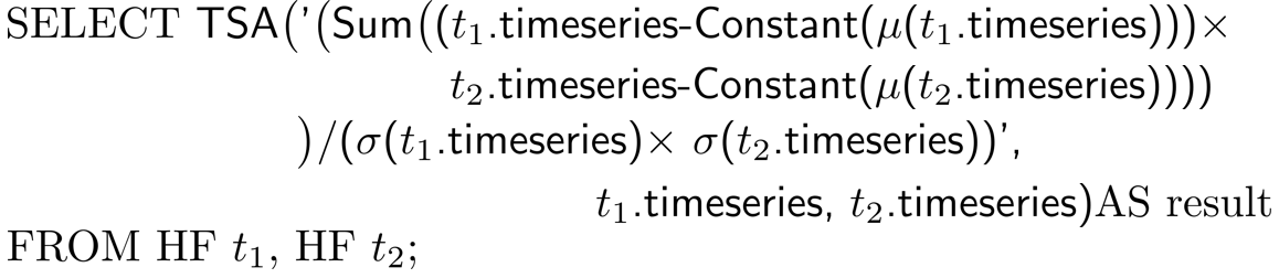
Queries. The SQL query computing the correlation TSA for all the time series pairs in HF is shown in Figure 19. The SQL queries on the other three datasets are similar by change the table HF to HI, HB and HA respectively.

	$\displaystyle\varepsilon$	$\displaystyle=\Big\|\sum_{i=a}^{b}\bm{T}_{1}[i]\bm{T}_{2}[i]-\sum_{i=a}^{b}f^{}_{T_{1}}(i)f^{}_{T_{2}}(i)\Big\|$
		$\displaystyle=\Big\|\sum_{i=1}^{k}\Big(\sum_{j=a_{i}}^{b_{i}}\bm{T}_{1}[i]\bm{T}_{2}[i]-\sum_{j=a_{i}}^{b_{i}}f^{}_{T_{1}}(i)f^{}_{T_{2}}(i)\Big)\Big\|$
		$\displaystyle=\Big\|\sum_{i=1}^{k}\Big(\langle\bm{\varepsilon}_{T_{1}^{i}},f^{}_{T_{2}^{i}}\rangle+\langle\bm{\varepsilon}_{T_{2}^{i}},f^{}_{T_{1}^{i}}\rangle+\langle\bm{\varepsilon}_{T_{1}^{i}},\bm{\varepsilon}_{T_{2}^{i}}\rangle\Big)\Big\|$
		$\displaystyle\leq\Big\|\sum_{i=1}^{k}\langle\bm{\varepsilon}_{T_{1}^{i}},f^{}_{T_{2}^{i}}\rangle\Big\|+\Big\|\sum_{i=1}^{k}\langle\bm{\varepsilon}_{T_{2}^{i}},f^{}_{T_{1}^{i}}\rangle\Big\|+\Big\|\sum_{i=1}^{k}\langle\bm{\varepsilon}_{T_{1}^{i}},\bm{\varepsilon}_{T_{2}^{i}}\rangle\Big\|$
		$\displaystyle\leq\sum_{i=1}^{k}\Big(\\|\varepsilon_{T_{1}^{i}}\\|_{2}\\|\varepsilon_{T_{2}^{i}}\\|_{2}+\\|\varepsilon_{T_{1}^{i}}\\|_{2}\\|f_{T_{2}^{i}}\\|_{2}+\\|f_{T_{1}^{i}}\\|_{2}\\|\varepsilon_{T_{2}^{i}}\\|_{2}\Big)$

	Generated Error Measures
	$\\|\varepsilon_{T}\\|_{2}$	$\\|f_{T}\\|_{2}$	$\gamma_{T}$
$\bm{T}=\bm{T_{1}+T_{2}}$	$\\|\varepsilon_{T_{1}}\\|_{2}+\\|\varepsilon_{T_{2}}\\|_{2}$	$\\|f_{T_{1}}\\|_{2}+\\|f_{T_{2}}\\|_{2}$	$\gamma_{T_{1}}+\gamma_{T_{2}}$
$\bm{T}=\bm{T_{1}-T_{2}}$	$\\|\varepsilon_{T_{1}}\\|_{2}+\\|\varepsilon_{T_{2}}\\|_{2}$	$\\|f_{T_{1}}\\|_{2}+\\|f_{T_{2}}\\|_{2}$	$\gamma_{T_{1}}+\gamma_{T_{2}}$
$\bm{T}=\bm{T_{1}\times T_{2}}$	$\\|\varepsilon_{T_{1}}\\|_{2}\\|\varepsilon_{T_{2}}\\|_{2}$	$\\|f_{T_{1}}\\|_{2}\\|f_{T_{2}}\\|_{2}$	$\\|\varepsilon_{T_{1}}\\|_{2}\\|\varepsilon_{T_{2}}\\|_{2}$
	$+\\|\varepsilon_{T_{1}}\\|_{2}\\|f_{T_{2}}\\|_{2}$		$\\|\varepsilon_{T_{1}}\\|_{2}\\|\varepsilon_{T_{2}}\\|_{2}$
	$+\\|\varepsilon_{T_{2}}\\|_{2}\\|f_{T_{2}}\\|_{2}$		$+\\|\varepsilon_{T_{1}}\\|_{2}\\|f_{T_{2}}\\|_{2}$
			$+\\|\varepsilon_{T_{2}}\\|_{2}\\|f_{T_{2}}\\|_{2}$

		$\displaystyle\|\langle\bm{\varepsilon}_{T_{1}},\bm{f}_{T_{2}}\rangle\|=\big\|\sum\limits_{i=1}^{k_{1}}\langle\bm{\varepsilon}_{T_{1}}\|_{[a_{i},b_{i}]},\bm{f}_{T_{2}}\|_{[a_{i},b_{i}]}\rangle\big\|$
		$\displaystyle=\Big\|\sum\limits_{i=1}^{k_{1}}\Big(\overbrace{\langle\bm{\varepsilon}_{T_{1}}\|_{[a_{1}^{i},b_{1}^{i}]},f^{}_{T_{1}^{i}}\rangle}^{=0}+\langle\bm{\varepsilon}_{T_{1}}\|_{[a_{1}^{i},b_{1}^{i}]},\bm{f}_{T_{2}}\|_{[a_{1}^{i},b_{1}^{i}]}-f^{}_{T_{1}^{i}}\rangle\Big)\Big\|$
		$\displaystyle\leq\sum\limits_{i=1}^{k_{1}}\Big\|\Big(\langle\bm{\varepsilon}_{T_{1}}\|_{[a_{1}^{i},b_{1}^{i}]},\bm{f}_{T_{2}}\|_{[a_{1}^{i},b_{1}^{i}]}-f^{*}_{T_{1}^{i}}\rangle\Big)\Big\|$
		$\displaystyle\leq\sum\limits_{i=1}^{k_{1}}\big\\|\bm{\varepsilon}_{T_{1}}\|_{[a_{1}^{i},b_{1}^{i}]}\big\\|_{2}\big\\|\bm{f}_{T_{2}}\|_{[a_{1}^{i},b_{1}^{i}]}-f^{*}_{T_{1}^{i}}\big\\|_{2}$
		$\displaystyle=\sum\limits_{i=1}^{k_{1}}\\|\varepsilon_{T_{1}^{i}}\\|_{2}\\|\bm{f}_{T_{2}}\|_{[a_{1}^{i},b_{1}^{i}]}-f^{*}_{T_{1}^{i}}\\|_{2}$

		$\displaystyle\\|\bm{f_{T_{2}}\|_{[a_{1}^{i},b_{1}^{i}]}-f^{*}_{T_{1}^{i}}}\\|_{2}=$
		$\displaystyle\Big(\sum_{j\in\Pi_{T_{2},[a_{1}^{i},b_{1}^{i}]}}\\|\bm{f_{T_{2}}\|_{[a_{1}^{i},b_{1}^{i}]\cap[a_{2}^{j},b_{2}^{j}]}}-\bm{f^{*}_{T_{1}^{i}}\|_{[a_{1}^{i},b_{1}^{i}]\cap[a_{2}^{j},b_{2}^{j}]}}\\|_{2}^{2}\Big)^{\frac{1}{2}}$
		$\displaystyle=\Big(\sum_{j\in\Pi_{T_{2},[a_{i},b_{i}]}}\\|\Psi([a_{2}^{i},b_{2}^{i}],[a_{1}^{i},b_{1}^{i}]\cap[a_{2}^{j},b_{2}^{j}])f^{*}_{T_{2}^{j}}$
		$\displaystyle~~~~~~-\Psi([a_{1}^{i},b_{1}^{i}],[a_{1}^{i},b_{1}^{i}]\cap[a_{2}^{j},b_{2}^{j}])f^{*}_{T_{1}^{i}}\\|_{2}^{2}\Big)^{\frac{1}{2}}$