Hierarchical Majoranas in a Programmable Nanowire Network

Zhi-Cheng Yang Affiliation: Physics Department, Boston University, Boston, Massachusetts 02215, USA Thomas Iadecola Affiliation: Joint Quantum Institute and Condensed Matter Theory Center, Department of Physics, University of Maryland, College Park, Maryland 20742, USA Claudio Chamon Affiliation: Physics Department, Boston University, Boston, Massachusetts 02215, USA Christopher Mudry Affiliation: Condensed Matter Theory Group, Paul Scherrer Institute, CH-5232 Villigen PSI, Switzerland

August 24, 2026

Abstract

We propose a hierarchical architecture for building “logical” Majorana zero modes using “physical” Majorana zero modes at the Y-junctions of a hexagonal network of semiconductor nanowires. Each Y-junction contains three “physical” Majoranas, which hybridize when placed in close proximity, yielding a single effective Majorana mode near zero energy. The hybridization of effective Majorana modes on neighboring Y-junctions is controlled by applied gate voltages on the links of the honeycomb network. This gives rise to a tunable tight-binding model of effective Majorana modes. We show that selecting the gate voltages that generate a Kekulé vortex pattern in the set of hybridization amplitudes yields an emergent “logical” Majorana zero mode bound to the vortex core. The position of a logical Majorana can be tuned adiabatically, without moving any of the “physical” Majoranas or closing any energy gaps, by programming the values of the gate voltages to change as functions of time. A nanowire network supporting multiple such “logical” Majorana zero modes provides a physical platform for performing adiabatic non-Abelian braiding operations in a fully controllable manner.

I Introduction

Topological qubits offer stronger resistance to decoherence by storing quantum information non-locally. This property is a driving motivation behind theoretical studies of topological quantum computation. [1] Majorana zero modes (MZMs), for instance, make up half-a-qubit, thereby allowing the coding of qubits non-locally in two far-away Majoranas. There has been a number of experimental setups proposed to realize MZMs in condensed matter systems. [2, 3] One approach aims at engineering Hamiltonians with effective $p$ -wave superconductivity by proximitizing an $s$ -wave superconductor to a semiconductor nanowire with strong spin-orbit coupling, [4, 5, 6, 7, 8, 9, 10] or a topological insulator. [11, 12, 13, 14] Such hybrid systems typically host MZMs at the endpoints or boundaries of the system. Recently, the theoretically predicted quantized zero-bias conductance peak at $2e^{2}/h$ in the presence of MZMs has been observed in indium antimonide semiconductor nanowires covered with an aluminium superconducting shell. [15]

Refer to caption — Figure 1: (a) Hierarchy of Majorana zero modes (MZMs). We start from an array of Majorana nanowires, depicted as the black links of a honeycomb lattice. Each nanowire furnishes three “physical” QMZMs (green circles in the inset) that hybridize locally, leaving one QMZM at each $Y$ -junction (blue circle in the inset). The resulting effective QMZMs reside on the sites of a honeycomb lattice (blue and red circles). An array of gates (grey “plungers”) provides tunable hybridization amplitudes for the effective QMZMs. Writing a particular pattern of gate voltages gives rise to a Kekulé vortex that binds an emergent “logical” MZM (purple density profile). The position $\bm{R}(t)$ of the emergent MZM is arbitrary and can be tuned continuously as a function of time, so that multiple “logical” MZMs can be braided adiabatically. Inset: Definition of the hexagonal lattice in terms of the two triangular sublattices $\Lambda^{\,}_{A}$ and $\Lambda^{\,}_{B}$ , with the nearest-neighbor vectors $\bm{s}^{\,}_{\alpha}$ , $\alpha=\mathtt{x},\mathtt{y},\mathtt{z}$ . (b) Controlling the overlap between adjacent effective QMZMs with a gate voltage $V^{\,}_{\mathrm{g}}$ . The Majorana wavefunctions (purple) decay exponentially across the length of the nanowire with a decay length that scales inversely with the topological nanowire gap $\Delta^{\,}_{\mathrm{nw}}$ . Increasing $V^{\,}_{\mathrm{g}}$ from $V^{\,}_{\mathrm{g},1}$ to $V^{\,}_{\mathrm{g},2}>V^{\,}_{\mathrm{g},1}$ decreases the nanowire gap, thereby increasing the wavefunction decay length, and with it the overlap between the two effective QMZMs (compare solid and dashed curves).

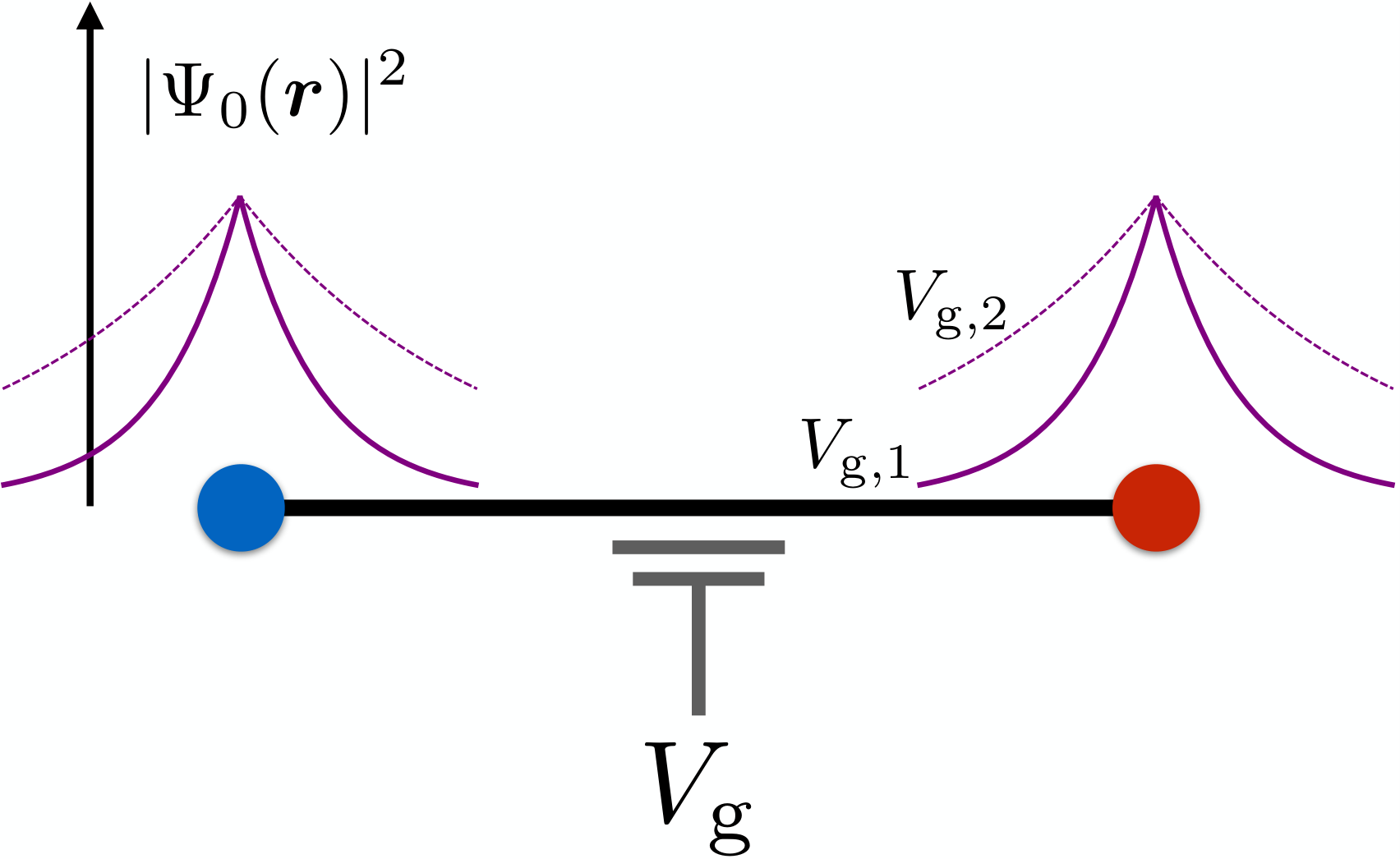
Despite this progress, there remains the question of how to braid MZMs once they are realized experimentally. For example, many proposals for braiding MZMs involve gradually moving microscopic MZMs by applying an array of gates to a single nanowire [16]. There also exists alternative braiding protocols such as coupling to magnetic fluxes [17] and measurement-only approaches [18]. In this work, we shall propose a scheme where braiding of MZMs can be implemented without violating the adiabatic hypothesis. The building blocks of our proposal are Majorana nanowires, i.e., semiconductor nanowires supporting Majorana modes bound to their endpoints at sufficiently low temperatures. However, the “logical” MZMs that are braided are not these elementary Majorana modes residing at the endpoints of the nanowires. Rather, they are emergent zero modes bound to point topological defects that can be programmed by gating the nanowires. These emergent zero modes live in two spatial dimensions, in contrast to 1D wires where the braiding statistics is intrinsically ill-defined. The “logical” MZMs are hierarchical, in the sense that they emerge by coupling together a set of Majorana modes that are themselves the result of the topological state of matter realized in each nanowire. The hierarchy of Majorana zero modes that are used in this work is depicted schematically in Fig. 1(a).

The hierarchical construction of the “logical” MZMs starts from a set of Majorana nanowires. Since each nanowire is of finite size, the Majorana modes at its endpoints hybridize weakly and split from zero energy. We call such a Majorana mode a quasi-Majorana zero mode (QMZM). Imagine placing one of the Majorana nanowires on each bond of a honeycomb lattice. At each vertex of the honeycomb lattice, where three nanowires form a Y-junction, three QMZMs hybridize strongly as their wavefunctions have large overlaps. This hybridization results in two QMZMs splitting away from zero energy by an amount much larger than the energy splitting of the QMZMs bound to the endpoints of a single nanowire, leaving a single effective QMZM at each site of the honeycomb lattice. This is the next level of the hierarchy. Now, imagine reducing the length of the Majorana nanowires making up the bonds of the honeycomb lattice. The increase of the overlap between these effective QMZMs will then be captured by a tight-binding model for Majorana modes hopping on the honeycomb lattice. If we assume translation invariant nearest-neighbor hopping amplitudes, there arises a gapped liquid with two massive Majorana cones very much as one finds in Kitaev’s honeycomb model in the presence of a magnetic field, [19] or in other lattices in the presence of quartic Majorana interactions. [20]

Another gap, which allows for the formation and manipulation of “logical” MZMs, can then be opened by giving the hopping amplitudes a Kekulé pattern. In practice, this can be done by applying voltages on the individual Majorana nanowires, which modulates the hybridization of nearest-neighbor effective QMZMs. To see how, recall that the topological gap $\Delta^{\,}_{\mathrm{nw}}$ in a Majorana nanowire decreases when a gate voltage $V^{\,}_{\mathrm{g}}$ is applied, thereby increasing the hybridization. [4, 5, 6, 7] Decreasing the size of the topological gap increases the decay length of the QMZMs, thereby increasing the overlap of their wavefunctions, see Fig. 1(b). Thus, by programming the set of gate voltages applied to every bond, one can exercise control over every hopping amplitude in the effective tight-binding model.

Furthermore, one can program these hopping amplitudes in a position-dependent manner so as to “write” an arbitrary number $v$ of Kekulé vortices into the system. This is achieved by modulating the gate voltages as $V^{\,}_{\mathrm{g}}\to V^{\,}_{\mathrm{g}}+\delta V^{\,}_{\mathrm{g}\,\bm{r},\alpha}$ , where

\delta V^{\,}_{\mathrm{g}\,\bm{r},\alpha}\,\raisebox{0.85pt}{.}\hskip-2.78pt\raisebox{2.85pt}{.}\!\!=\,V^{\,}_{0}\,\cos\left(\bm{K}^{\,}_{+}\cdot\bm{s}^{\,}_{\alpha}+(\bm{K}^{\,}_{+}-\bm{K}^{\,}_{-})\cdot\bm{r}+\sum_{n=1}^{v}q^{\,}_{n}\,\mathrm{arg}\left(\bm{r}-\bm{R}^{\,}_{n}\right)\right).

(1)

Here, $\bm{r}$ is a point in one of the triangular sublattices of the honeycomb lattice, $\bm{s}^{\,}_{\alpha}$ ( $\alpha=\mathtt{x},\mathtt{y},\mathtt{z}$ ) are the nearest-neighbor vectors connecting to the other sublattice (see Fig. 1), $\bm{K}^{\,}_{+}=-\bm{K}^{\,}_{-}$ are the corners of the Brillouin zone of the honeycomb lattice. The vorticities $q^{\,}_{n}=\pm 1$ ( $n=1,\dots,v$ ) and positions $\bm{R}^{\,}_{n}$ are here merely parameters that can be tuned at will. Kekulé vortices have been shown to bind zero-energy modes in graphene, [21, 22] analogs of which also appear in photonic crystals. [23] Similar physics arises here, with the crucial distinction that the zero modes are now of Majorana nature, owing to the fact that the underlying tight-binding model is one of Majoranas. It is the MZMs localized near the core of each vortex that we shall call the “logical” MZMs, which constitute the final level of the hierarchy. Because the positions $\bm{R}_{n}$ of the vortices are merely parameters, they can be tuned simply by changing the voltages on each wire as a function of time, like addressing pixels on a screen. Therefore, in a system with multiple vortices, this scheme would allow one to move and braid the logical MZMs adiabatically.

The rest of the paper is organized as follows. We present the realization with Majorana nanowires in Sec. II of an analogue of a $p+\mathrm{i}p$ superconductor belonging to the symmetry class D. We determine the conditions under which the Kekulé dimerization controls the gap. We define a scaling limit that allows one to derive a simple model of free Majoranas with nearest-neighbor hopping amplitudes on a honeycomb lattice in Sec. III. In this scaling limit, the low-energy effective theory has higher symmetry, belonging to symmetry class BDI. We explicitly solve for the MZM bound to a Kekulé vortex. We further show that the Kekulé vortices indeed have the braiding statistics of MZMs. In Sec. IV, we demonstrate numerically the emergence of an MZM bound to the core of a Kekulé vortex away from the scaling limit. Section V discusses possible experimental measurement schemes for the emergent MZMs and demonstrates the feasibility of our setup using realistic experimental parameters. We conclude with a summary and outlook for future directions in Sec. VI.

II Realization with Majorana nanowires

The building block that we shall use in this paper is a nanowire which at low temperatures supports a topological superconducting gap $\Delta^{\,}_{\mathrm{nw}}$ . Because of the topological gap $\Delta^{\,}_{\mathrm{nw}}$ , the nanowire hosts a pair of QMZMs at its endpoints when superconducting. We shall call such a nanowire a “Majorana nanowire.”

The main idea of this paper is to imagine that each nearest-neighbor bond of the honeycomb lattice is realized by a Majorana nanowire. There are two energy scales in the problem: a hybridization ${{U}}$ and a hopping amplitude ${{t}}$ , as we now explain.

On the one hand, three Majorana nanowires must meet at the sites of the honeycomb lattice, thereby realizing a Y-junction of Majorana nanowires, as shown in Fig. 2. Effectively (i.e., below the energy gap $\Delta^{\,}_{\mathrm{nw}}$ of an isolated Majorana nanowire), we have three flavors of QMZMs on each site of the honeycomb lattice. The pairwise hybridization among the three QMZMs will split their quasidegeneracy by an energy scale $|{{U}}|$ . Then, only one QMZM remains below the energy scale $|{{U}}|$ on any given Y-junction (site of the honeycomb lattice). Thus, each Y-junction effectively contributes a single emergent Majorana mode.

On the other hand, the pair of QMZMs bound to the two ends of a Majorana nanowire are split away from zero energy by the energy scale ${{t}}$ that results from the overlap of their wavefunctions. This hybridization increases as each Majorana nanowire is shortened, inducing a nearest-neighbor hopping amplitude ${{t}}$ for the three pairs of QMZMs localized on nearest-neighbor Y-junctions of Majorana nanowires.

Hence, working at energies below the topological gap $\Delta^{\,}_{\mathrm{nw}}$ of a Majorana nanowire, we have outlined the construction of an effective six-band tight-binding model on the honeycomb lattice using Majorana nanowires. Below we shall discuss this construction in more detail.

Figure 3: Representation of the trimer limit defined by the ground state of Hamiltonian (3). The MZMs at each Y-junction are represented by green dots. Their pairwise hybridization

{{U}}

is represented by directed bonds arranged along the edges of a triangle. The blue and red triangles encircles sites from sublattices

\Lambda^{\,}_{A}

and

\Lambda^{\,}_{B}

, respectively. The hybridization energy scale for blue and red triangles is

{{U}}

. The pattern of arrows along the edges of each triangle defines the order in which two Majorana operators are to be multiplied with the convention that

{{U}}

is positive for this order of multiplication.

II.1 Trimer limit ( ${{U}}\neq 0$ , ${{t}}=0$ )

Consider a honeycomb lattice $\Lambda$ made of two interpenetrating triangular lattices $\Lambda^{\,}_{A}$ and $\Lambda^{\,}_{B}$ . We shall label the bonds of the honeycomb lattice by $\alpha=\mathtt{x},\mathtt{y},\mathtt{z}$ depending on their orientations, as shown in Fig. 2. Each bond of the honeycomb lattice realizes a Majorana nanowire. We shall thus associate to each bond of the honeycomb lattice a pair of Majorana operators as depicted in Fig. 2. If the label $S=A,B$ distinguishes between the triangular sublattices $\Lambda^{\,}_{A}$ and $\Lambda^{\,}_{B}$ , and if the label $j$ stands for a site from $\Lambda^{\,}_{S}$ , then the Majorana algebra reads

	$\left\{\hat{\gamma}^{\alpha}_{S,j},\hat{\gamma}^{\alpha^{\prime}}_{S^{\prime},j^{\prime}}\right\}=2\delta^{\,}_{\alpha,\alpha^{\prime}}\delta^{\,}_{S,S^{\prime}}\delta^{\,}_{j,j^{\prime}}$	(2a)
with the Majorana reality condition
	$\hat{\gamma}^{\alpha{\dagger}}_{S,j}=\hat{\gamma}^{\alpha}_{S,j}.$	(2b)

These Majorana operators stand at the first level of the hierarchy.

The trimer limit occurs for ${{t}}=0$ . The Hamiltonian describing this limit is

\displaystyle\widehat{H}^{\,}_{\mathrm{trimer}}\,\raisebox{0.85pt}{.}\hskip-2.78pt\raisebox{2.85pt}{.}\!\!=\,

\displaystyle\!\!\!\sum_{S=A,B}\sum_{j\in\Lambda^{\,}_{S}}\!\mathrm{i}{{U}}\!\left(\hat{\gamma}^{\mathtt{x}}_{S,j}\,\hat{\gamma}^{\mathtt{y}}_{S,j}\!+\!\hat{\gamma}^{\mathtt{y}}_{S,j}\,\hat{\gamma}^{\mathtt{z}}_{S,j}\!+\!\hat{\gamma}^{\mathtt{z}}_{S,j}\,\hat{\gamma}^{\mathtt{x}}_{S,j}\right).

(3)

We represent in Fig. 3 the trimer limit as a decorated honeycomb lattice. Hybridization within each Y-junction is represented by a directed arrow relating a pair of MZMs. The direction of the arrows along the edges of each triangle defines the order in which two Majorana operators are to be multiplied. It fixes the sign of the hybridization ${{U}}$ to be positive along the arrow. Reversing the chirality of the red or blue triangles thus amounts to reversing the sign of ${{U}}$ .

Hamiltonian (3) is the sum over $S=A,B$ and $j\in\Lambda^{\,}_{S}$ of the pairwise commuting operators

	$\mathrm{i}{{U}}\left(\hat{\gamma}^{\mathtt{x}}_{S,j}\,\hat{\gamma}^{\mathtt{y}}_{S,j}+\hat{\gamma}^{\mathtt{y}}_{S,j}\,\hat{\gamma}^{\mathtt{z}}_{S,j}+\hat{\gamma}^{\mathtt{z}}_{S,j}\,\hat{\gamma}^{\mathtt{x}}_{S,j}\right).$	(4a)
As each one of these operators has the three single-particle eigenvalues
	$-\sqrt{3}\,{{U}},\qquad 0,\qquad+\sqrt{3}\,{{U}},$	(4b)
with the Majorana zero mode
	$\hat{\eta}\,\raisebox{0.85pt}{.}\hskip-2.78pt\raisebox{2.85pt}{.}\!\!=\,\frac{1}{\sqrt{3}}\left(\hat{\gamma}^{\mathtt{x}}_{S,j}+\hat{\gamma}^{\mathtt{y}}_{S,j}+\hat{\gamma}^{\mathtt{z}}_{S,j}\right),$	(4c)

Hamiltonian (3) supports three doubly-degenerate flat bands with the single-particle energies (4b), respectively.

Figure 4: Representation of the dimer limit defined by the ground state of Hamiltonian (5a). The arrows specify the order in which Majorana operators (the green dots) enter Hamiltonian (5a), with the convention that operators on sublattice

\Lambda^{\,}_{A}

are to the left of operators from sublattice

\Lambda^{\,}_{B}

along an arrow. With this convention, the hopping amplitude

t

is positive along an arrow.

II.2 Dimer limit ( ${{t}}\neq 0$ , ${{U}}=0$ )

The dimer limit occurs for ${{U}}=0$ . The Hamiltonian describing this limit is

	$\widehat{H}^{\,}_{\mathrm{dimer}}\,\raisebox{0.85pt}{.}\hskip-2.78pt\raisebox{2.85pt}{.}\!\!=\,\sum_{j\in\Lambda^{\,}_{A}}\sum_{\alpha=\mathtt{x},\mathtt{y},\mathtt{z}}\mathrm{i}{{t}}\,\hat{\gamma}^{\alpha}_{A,j}\,\hat{\gamma}^{\alpha}_{B,j+\bm{s}^{\,}_{\alpha}}.$	(5a)
Here, $\bm{s}^{\,}_{\alpha}$ are the unit vectors connecting the three sites in $\Lambda^{\,}_{B}$ that are nearest-neighbor to a site in $\Lambda^{\,}_{A}$ , i.e.,
	$\bm{s}^{\,}_{\mathtt{z}}\,\raisebox{0.85pt}{.}\hskip-2.78pt\raisebox{2.85pt}{.}\!\!=\,\begin{pmatrix}0\\ -1\end{pmatrix},\quad\bm{s}^{\,}_{\mathtt{x}}\,\raisebox{0.85pt}{.}\hskip-2.78pt\raisebox{2.85pt}{.}\!\!=\,\begin{pmatrix}+\sqrt{3}/2\\ 1/2\end{pmatrix},\quad\bm{s}^{\,}_{\mathtt{y}}\,\raisebox{0.85pt}{.}\hskip-2.78pt\raisebox{2.85pt}{.}\!\!=\,\begin{pmatrix}-\sqrt{3}/2\\ 1/2\end{pmatrix}.$	(5b)

One may represent this Hamiltonian as is done in Fig. 4. The energy scale ${{t}}$ results from the finite lengths of Majorana nanowires, which allows the pair of wavefunctions of the QMZMs bound to the two ends of the semiconductor nanowire to have a nonvanishing overlap. This overlap leads to a splitting of their energies away from $0$ by the amount $\pm|{{t}}|$ .

Hamiltonian (5a) is the sum over $j\in\Lambda^{\,}_{A}$ and $\alpha=\mathtt{x},\mathtt{y},\mathtt{z}$ of the pairwise commuting operators

	$\mathrm{i}{{t}}\,\hat{\gamma}^{\alpha}_{A,j}\,\hat{\gamma}^{\alpha}_{B,j+\bm{s}^{\,}_{\alpha}}.$	(6a)
As each one of these operators has the two single-particle eigenvalues
	$-\|{{t}}\|,\qquad+\|{{t}}\|$	(6b)

Hamiltonian (5a) supports two triply-degenerate flat bands with the single-particle energies (6b), respectively. The single-particle energies (6b) correspond to the fermionic state

\hat{c}^{\alpha{\dagger}}_{j}|0\rangle\,\raisebox{0.85pt}{.}\hskip-2.78pt\raisebox{2.85pt}{.}\!\!=\,\frac{1}{2}\left(\hat{\gamma}^{\alpha}_{A,j}-\mathrm{i}\,\hat{\gamma}^{\alpha}_{B,j+\bm{s}^{\,}_{\alpha}}\right)\,|0\rangle,\qquad\hat{c}^{\alpha}_{j}|0\rangle\,\raisebox{0.85pt}{.}\hskip-2.78pt\raisebox{2.85pt}{.}\!\!=\,0,

(7)

being empty or occupied, respectively. There is no zero mode in the dimer limit.

II.3 Reversal of time

We shall define the action of time reversal by the rules

\mathrm{i}\mapsto-\mathrm{i},\qquad\hat{\gamma}^{\alpha}_{A,j}\mapsto+\hat{\gamma}^{\alpha}_{A,j},\qquad\hat{\gamma}^{\alpha}_{B,j+\bm{s}^{\,}_{\alpha}}\mapsto-\hat{\gamma}^{\alpha}_{B,j+\bm{s}^{\,}_{\alpha}}.

(8)

The motivation for this definition is that we would like to interpret

\hat{c}^{\alpha}_{A,j}\,\raisebox{0.85pt}{.}\hskip-2.78pt\raisebox{2.85pt}{.}\!\!=\,\frac{1}{2}\left(\hat{\gamma}^{\alpha}_{A,j}+\mathrm{i}\,\hat{\gamma}^{\alpha}_{B,j+\bm{s}^{\,}_{\alpha}}\right)

(9)

as a fermion operator localized on the directed bond $\langle j\in\Lambda^{\,}_{A},j+\bm{s}^{\,}_{\alpha}\in\Lambda^{\,}_{B}\rangle$ of the honeycomb lattices that is left invariant by the operation of time reversal.

One verifies that Hamiltonian (5a) is even under reversal of time while Hamiltonian (3) is odd under reversal of time, i.e.,

\widehat{H}^{\,}_{\mathrm{dimer}}\mapsto+\widehat{H}^{\,}_{\mathrm{dimer}},\qquad\widehat{H}^{\,}_{\mathrm{trimer}}\mapsto-\widehat{H}^{\,}_{\mathrm{trimer}}.

(10)

Although $\widehat{H}^{\,}_{\mathrm{trimer}}$ is odd under time reversal, the zero-energy flat band transforms trivially whereas the finite-energy bands are interchanged.

II.4 Hamiltonian for the nanowire network

When both ${{U}}\neq 0$ and ${{t}}\neq 0$ , we can write the noninteracting Hamiltonian in momentum space as

	$\begin{split}\widehat{H}^{\,}_{\mathrm{wire}}\,\raisebox{0.85pt}{.}\hskip-2.78pt\raisebox{2.85pt}{.}\!\!=\,&\,\widehat{H}^{\,}_{\mathrm{trimer}}+\widehat{H}^{\,}_{\mathrm{dimer}}=\int\limits^{\,}_{\Omega^{\mathrm{K}}_{\mathrm{BZ}}}\mathrm{d}^{3}\bm{k}\,\widehat{\Psi}^{{\dagger}}_{\bm{k}}\,\mathcal{H}^{\,}_{\mathrm{wire}}\,\widehat{\Psi}^{\,}_{\bm{k}},\end{split}$	(11a)
with the spinor
	$\widehat{\Psi}^{{\dagger}}_{\bm{k}}=\begin{pmatrix}\hat{\gamma}^{\mathtt{x}}_{A,\bm{k}}&\hat{\gamma}^{\mathtt{y}}_{A,\bm{k}}&\hat{\gamma}^{\mathtt{z}}_{A,\bm{k}}&\hat{\gamma}^{\mathtt{x}}_{B,\bm{k}}&\hat{\gamma}^{\mathtt{y}}_{B,\bm{k}}&\hat{\gamma}^{\mathtt{z}}_{B,\bm{k}}\end{pmatrix}$	(11b)
and the single-particle Hamiltonian
	$\mathcal{H}^{\,}_{\mathrm{wire}}=\begin{pmatrix}0&+\mathrm{i}{{U}}/2&-\mathrm{i}{{U}}/2&+\frac{\mathrm{i}{{t}}}{2}\,e^{\mathrm{i}\bm{k}\cdot\bm{s}^{\,}_{\mathtt{x}}}&0&0\\ -\mathrm{i}{{U}}/2&0&+\mathrm{i}{{U}}/2&0&+\frac{\mathrm{i}{{t}}}{2}\,e^{\mathrm{i}\bm{k}\cdot\bm{s}^{\,}_{\mathtt{y}}}&0\\ +\mathrm{i}{{U}}/2&-\mathrm{i}{{U}}/2&0&0&0&+\frac{\mathrm{i}{{t}}}{2}\,e^{\mathrm{i}\bm{k}\cdot\bm{s}^{\,}_{\mathtt{z}}}\\ -\frac{\mathrm{i}{{t}}}{2}\,e^{-\mathrm{i}\bm{k}\cdot\bm{s}^{\,}_{\mathtt{x}}}&0&0&0&+\mathrm{i}{{U}}/2&-\mathrm{i}{{U}}/2\\ 0&-\frac{\mathrm{i}{{t}}}{2}\,e^{-\mathrm{i}\bm{k}\cdot\bm{s}^{\,}_{\mathtt{y}}}&0&-\mathrm{i}{{U}}/2&0&+\mathrm{i}{{U}}/2\\ 0&0&-\frac{\mathrm{i}{{t}}}{2}\,e^{-\mathrm{i}\bm{k}\cdot\bm{s}^{\,}_{\mathtt{z}}}&+\mathrm{i}{{U}}/2&-\mathrm{i}{{U}}/2&0\end{pmatrix}.$	(11c)

The single-particle Hamiltonian (11c) is of Bogoliubov-de Gennes (BdG) form. This is to say that out of its six Majorana bands, three have positive single-particle energies, three have negative single single-particle energies, and there exists an antiunitary transformation such that the six bands can be organized into three pairs such that for any one of these three pairs the Majorana band with positive single-particle energy maps to the Majorana band with negative single-particle energy and vice versa under the antiunitary transformation.

When $|{{U}}/{{t}}|\ll 1$ , the two flat bands of $\widehat{H}^{\,}_{\mathrm{dimer}}$ acquire a dispersion with a bandwidth that is controlled by $|{{U}}|$ . Both bands are topologially trivial. We will not consider this limit anymore in the paper.

When $|{{t}}/{{U}}|\ll 1$ , the zero-energy modes (4c) of $\widehat{H}^{\,}_{\mathrm{trimer}}$ that are localized on the sites of the honeycomb lattice get hybridized by $\widehat{H}^{\,}_{\mathrm{dimer}}$ . More precisely, the twofold degenerate flat band in the Brillouin zone $\Omega^{\,}_{\mathrm{BZ}}$ arising from the zero mode $\hat{\eta}$ defined in Eq. (4c) when ${{t}}/{{U}}=0$ turns into two bands related by particle-hole symmetry. The bandwidth for this pair of Majorana bands is of order $|{{t}}|$ . These emergent low-energy Majorana modes realize the second level of the hierarchy of Majoranas. The limit $|{{U}}|\gg|{{t}}|$ enforces the first hierarchical reduction in the number of effective Majorana modes. We now turn to a quantitative analysis of the band structure of the Hamiltonian (11c) in this limit.

In Fig. 5, we plot the band structure for ${{t}}/{{U}}=0.1$ with ${{U}}>{{t}}>0$ . We find that a gap opens at the corners of the Brillouin zone. We shall call this gap the Haldane gap. This terminology will be explained when we introduce the single-particle Hamiltonian (19) and show that it opens a spectral gap and endows Majorana bands with non-vanishing Chern numbers. A direct calculation of the eigenvalues at $\bm{K}^{\,}_{\pm}$ shows that the energies of the two bands at $\bm{K}^{\,}_{\pm}$ are given by

$\displaystyle\varepsilon^{\,}_{\pm}(\bm{K}^{\,}_{+})=$	$\displaystyle\,\varepsilon^{\,}_{\pm}(\bm{K}^{\,}_{-})$
$\displaystyle=$	$\displaystyle\,\pm\frac{1}{4}\left(\sqrt{3}\,{{U}}-\sqrt{3{{U}}^{2}+4{{t}}^{2}}\right)$
$\displaystyle\approx$	$\displaystyle\,\pm\frac{{{t}}^{2}}{2\sqrt{3}\,{{U}}}+\mathcal{O}\left(\frac{{{t}}^{4}}{{{U}}^{3}}\right).$	(12)

We thus find that the Haldane gap is of order ${{t}}^{2}/{{U}}$ and, as such, can be explained within second-order perturbation theory. Upon linearization of the single-particle Hamiltonian in the vicinity of $\bm{K}^{\,}_{\pm}$ , this gap can be interpreted as a Haldane mass that implements the microscopic breaking of time-reversal symmetry. [24]. The counterpart of this phase in the Kitaev’s honeycomb model is the non-Abelian topologically ordered phase stabilized by a magnetic field. [19]

When the system is perturbed by a Kekulé dimerization defined by

	$\delta\widehat{H}^{\,}_{\mathrm{dimer}}\,\raisebox{0.85pt}{.}\hskip-2.78pt\raisebox{2.85pt}{.}\!\!=\,\mathrm{i}\sum_{j\in\Lambda^{\,}_{A}}\sum_{\alpha=\mathtt{x},\mathtt{y},\mathtt{z}}\delta{{t}}_{j,\alpha}\,\hat{\gamma}^{\alpha}_{A,j}\,\hat{\gamma}^{\alpha}_{B,j+\bm{s}^{\,}_{\alpha}}$	(13a)
with the dimerization pattern [25]
	$\delta{{t}}^{\,}_{j,\alpha}\,\raisebox{0.85pt}{.}\hskip-2.78pt\raisebox{2.85pt}{.}\!\!=\,\Delta\,e^{\mathrm{i}\bm{K}^{\,}_{+}\cdot\bm{s}^{\,}_{\alpha}}\,e^{\mathrm{i}\bm{G}\cdot\bm{r}_{j}}+\mathrm{c.c.},$	(13b)
where the Kekulé amplitude
	$\Delta\,\raisebox{0.85pt}{.}\hskip-2.78pt\raisebox{2.85pt}{.}\!\!=\,\Delta^{\,}_{0}\,e^{\mathrm{i}\varphi},\qquad\Delta^{\,}_{0}\,\raisebox{0.85pt}{.}\hskip-2.78pt\raisebox{2.85pt}{.}\!\!=\,\|\Delta\|,\qquad\varphi\in[0,2\pi),$	(13c)
and
	$\bm{G}\,\raisebox{0.85pt}{.}\hskip-2.78pt\raisebox{2.85pt}{.}\!\!=\,\bm{K}^{\,}_{+}-\bm{K}^{\,}_{-}\equiv 2\bm{K}^{\,}_{+}\equiv-2\bm{K}^{\,}_{-}$	(13d)

is the momentum connecting the two valleys, such that $0<\Delta^{\,}_{0}\ll{{t}}^{2}/{{U}}$ , the band gap decreases until it vanishes when $\Delta^{\,}_{0}\sim{{t}}^{2}/{{U}}$ . When the Kekulé amplitude $\Delta^{\,}_{0}\gtrsim{{t}}^{2}/{{U}}$ , the gap is of Kekulé character [21]. This case is illustrated in Fig. 6. We stress that the Haldane and Kekulé gaps compete against each other, so they realize two distinct gapped phases separated by a gap-closing transition. [26] When the gap is of Haldane character, the bottom band has a Chern number $C=-1$ and there is a chiral mode propagating along the edge of a system with boundary. On the other hand, the Chern number vanishes across the phase transition when the gap is dominated by Kekulé dimerization, as shown in Fig. 6(e). In this phase, there is no chiral edge mode at the boundary of the system [27].

Figure 5: The pair of particle-hole symmetric bands with the lowest energies for Hamiltonian (11a) when

{{U}}/{{t}}=10

with

{{U}}>{{t}}>0

. A Haldane gap appears at the corners of the Brillouin zone

\Omega^{\,}_{\mathrm{BZ}}

(depicted in light blue). The magnitude of the Haldane gap follows from

\varepsilon^{\,}_{\pm}(\bm{K}^{\,}_{+})=\varepsilon^{\,}_{\pm}(\bm{K}^{\,}_{-})\approx\pm\frac{{{t}}^{2}}{2\sqrt{3}\,{{U}}}+\mathcal{O}({{t}}^{4}/{{U}}^{3})

. The energies are plotted in units of

t

II.5 Scaling limits

There is an interesting scaling limit of (11) consisting in taking the limit ${{U}}\to\infty$ holding ${{t}}$ fixed. In this limit, the hierarchy

	${{U}}>{{t}}>\frac{{{t}}}{{{U}}}\,{{t}}$	(14a)
becomes
	$\infty>{{t}}>0.$	(14b)

This limit sends to infinite energy the two pairs of particle-hole symmetric Majorana bands that are separated by an energy of order $2{{U}}$ [see Eqs. (4)]. It leaves a gapless pair of particle-hole symmetric Majorana bands with conical band crossing at the corners $\bm{K}^{\,}_{+}$ and $\bm{K}^{\,}_{-}$ of the Brillouin zone $\Omega^{\,}_{\mathrm{BZ}}$ . In this limit, time-reversal symmetry, as measured by the vanishing of the Haldane gap, is restored. This limit is useful as it allows one to treat in closed analytical form the effect of a Kekulé modulation of ${{t}}$ – in particular the effect of a vortex in the Kekulé modulation of ${{t}}$ – on the single-particle spectrum.

III Free Majoranas on a honeycomb lattice with Kekulé dimerization

We start by reviewing the properties of a tight-binding model for Majoranas hopping on the honeycomb lattice with nearest-neighbor hopping amplitudes. This model is motivated by the scaling limit ${{U}}\to\infty$ holding ${{t}}$ fixed that turns the hierarchy (14a) into the hierarchy (14b).

III.1 Gapless liquid phase with uniform hopping amplitudes

Consider a honeycomb lattice $\Lambda$ made of two interpenetrating triangular lattices $\Lambda^{\,}_{A}$ and $\Lambda^{\,}_{B}$ . We start with the operator $\hat{a}^{\,}_{\bm{r}}$ that either creates or annihilates a Majorana mode on the lattice site $\bm{r}$ , i.e.,

	$\{\hat{a}^{\,}_{\bm{r}},\hat{a}^{\,}_{\bm{r}^{\prime}}\}=2\delta^{\,}_{\bm{r},\bm{r}^{\prime}},\qquad\hat{a}^{{\dagger}}_{\bm{r}}=\hat{a}^{\,}_{\bm{r}},$	(15a)
for any pair of sites $\bm{r}$ and $\bm{r}^{\prime}$ . We endow these Majorana modes with the quantum dynamics specified by the single-particle Hamiltonian
	$\widehat{H}\,\raisebox{0.85pt}{.}\hskip-2.78pt\raisebox{2.85pt}{.}\!\!=\,\sum_{\bm{r}\in\Lambda^{\,}_{A}}\sum_{\alpha=\mathtt{x},\mathtt{y},\mathtt{z}}{{t}}\,\mathrm{i}\hat{a}^{\,}_{\bm{r}}\,\hat{a}^{\,}_{\bm{r}+\bm{s}^{\,}_{\alpha}}.$	(15b)

Without loss of generality, we choose the hopping amplitudes to be positive, ${{t}}>0$ . We have set the lattice spacing $\mathfrak{a}$ of the honeycomb lattice to unity, $\mathfrak{a}=1$ .

We observe that Majorana operators localized on sublattice $\Lambda^{\,}_{A}$ always appear to the left of Majorana operators localized on sublattice $\Lambda^{\,}_{B}$ in the Hamiltonian (15b). If we define the operation of time reversal by the rule

\mathrm{i}\mapsto-\mathrm{i},\qquad\hat{a}^{\,}_{\bm{r}}\mapsto+\hat{a}^{\,}_{\bm{r}},\qquad\hat{a}^{\,}_{\bm{r}+\bm{s}^{\,}_{\alpha}}\mapsto-\hat{a}^{\,}_{\bm{r}+\bm{s}^{\,}_{\alpha}},

(16)

we conclude that the Hamiltonian (15b) is invariant under reversal of time.

Hamiltonian (15b) is invariant under the translations that map the honeycomb lattice onto itself. Hence, we perform the Fourier transformation


		$\displaystyle\hat{a}^{\,}_{\bm{r}}\,=\!\!\raisebox{0.85pt}{.}\hskip-2.78pt\raisebox{2.85pt}{.}\,\frac{1}{\sqrt{N}}\sum_{\bm{k}\in\Omega^{\,}_{\mathrm{BZ}}}e^{\mathrm{i}\bm{k}\cdot\bm{r}}\hat{a}^{\,}_{A,\bm{k}},$	(17a)
		$\displaystyle\hat{a}^{\,}_{\bm{r}+\bm{s}^{\,}_{\alpha}}\,=\!\!\raisebox{0.85pt}{.}\hskip-2.78pt\raisebox{2.85pt}{.}\,\frac{1}{\sqrt{N}}\sum_{\bm{k}\in\Omega^{\,}_{\mathrm{BZ}}}e^{\mathrm{i}\bm{k}\cdot(\bm{r}+\bm{s}^{\,}_{\alpha})}\hat{a}^{\,}_{B,\bm{k}},$	(17b)
where $\Omega^{\,}_{\mathrm{BZ}}$ denotes the Brillouin zone of the triangular sublattice. Notice that since $\hat{a}^{\,}_{\bm{r}}$ is a Majorana operator, $\hat{a}^{{\dagger}}_{\bm{k}}$ and $\hat{a}^{\,}_{\bm{k}}$ are not independent,
	$\hat{a}^{{\dagger}}_{A,\bm{k}}=\hat{a}^{\,}_{A,-\bm{k}},\qquad\hat{a}^{{\dagger}}_{B,\bm{k}}=\hat{a}^{\,}_{B,-\bm{k}}.$		(17c)

If we introduce the two-component spinor

	$\hat{\gamma}^{{\dagger}}_{\bm{k}}\,\raisebox{0.85pt}{.}\hskip-2.78pt\raisebox{2.85pt}{.}\!\!=\,\begin{pmatrix}\hat{a}^{{\dagger}}_{A,\bm{k}}&\hat{a}^{{\dagger}}_{B,\bm{k}}\end{pmatrix},$	(18a)
Hamiltonian (15b) turns into
	$\widehat{H}=\sum_{\bm{k}\in\Omega^{\,}_{\mathrm{BZ}}}\hat{\gamma}^{{\dagger}}_{\bm{k}}\,\mathrm{i}\mathcal{A}^{\,}_{\bm{k}}\,\hat{\gamma}^{\,}_{\bm{k}},$	(18b)
where
	$\begin{split}\mathcal{H}^{\,}_{\bm{k}}\equiv&\,\mathrm{i}\mathcal{A}^{\,}_{\bm{k}}\\ \,\raisebox{0.85pt}{.}\hskip-2.78pt\raisebox{2.85pt}{.}\!\!=\,&\,\frac{\mathrm{i}}{2}\begin{pmatrix}0&+{{t}}\sum\limits_{\alpha=\mathtt{x},\mathtt{y},\mathtt{z}}e^{-\mathrm{i}\bm{k}\cdot\bm{s}^{\,}_{\alpha}}\\ -{{t}}\sum\limits_{\alpha=\mathtt{x},\mathtt{y},\mathtt{z}}e^{+\mathrm{i}\bm{k}\cdot\bm{s}^{\,}_{\alpha}}&0\end{pmatrix}.\end{split}$	(18c)

We observe that the symmetry under reversal of time defined by Eq. (16) is broken by adding to the single-particle Hamiltonian (18c) the traceless diagonal matrix

	$\mathcal{H}^{\mathrm{Hal}}_{\bm{k}}\,\raisebox{0.85pt}{.}\hskip-2.78pt\raisebox{2.85pt}{.}\!\!=\,\begin{pmatrix}+\Delta^{\mathrm{Hal}}_{\bm{k}}&0\\ 0&-\Delta^{\mathrm{Hal}}_{\bm{k}}\end{pmatrix},$	(19a)
where we demand that the so-called Haldane amplitude satisfies
	$\Delta^{\mathrm{Hal}}_{-\bm{k}}=-\Delta^{\mathrm{Hal}}_{+\bm{k}}$	(19b)

for any $\bm{k}$ in the Brillouin zone $\Omega^{\,}_{\mathrm{BZ}}$ .

Solving for

	$\sum\limits_{\alpha=\mathtt{x},\mathtt{y},\mathtt{z}}e^{+\mathrm{i}\bm{k}\cdot\bm{s}^{\,}_{\alpha}}=0$	(20a)
yields the two nodal points
	$\bm{K}^{\,}_{\pm}\,\raisebox{0.85pt}{.}\hskip-2.78pt\raisebox{2.85pt}{.}\!\!=\,\frac{4\pi}{3\sqrt{3}}\begin{pmatrix}\pm 1\\ 0\end{pmatrix}$	(20b)

at the corners $\bm{K}^{\,}_{\pm}$ of the Brillouin zone. Hence, the single-particle spectrum of the single-particle Hamiltonian (18c) is identical to that of graphene for spinless fermions at vanishing chemical potential by virtue of the Majorana representation in the second-quantized Hamiltonian (18b).

Adding the Haldane term (19) to the single-particle Hamiltonian (18c) opens a gap $2|\Delta^{\,}_{\bm{K}^{\,}_{+}}|>0$ , the so-called Haldane gap, at the corners $\bm{K}^{\,}_{\pm}$ of the Brillouin zone. The upper and lower bands carry opposite Chern numbers of magnitude $1$ when $2|\Delta^{\,}_{\bm{K}^{\,}_{+}}|>0$ . This Haldane gap is the counterpart to the gap (12).

If we focus on the low-energy physics near the two Majorana cones, we can write $\bm{k}=\bm{K}^{\,}_{\pm}+\bm{p}$ in the vicinity of $\bm{K}^{\,}_{\pm}$ and expand to leading order in $\bm{p}$ . The linearized Hamiltonian (15b) now takes the form


		$\displaystyle\widehat{H}\approx\frac{1}{2}\int\limits_{\Omega^{\,}_{\mathrm{BZ}}}\frac{\mathrm{d}^{2}\bm{p}}{(2\pi)^{2}}\,\widehat{\Upsilon}^{{\dagger}}(\bm{p})\,\mathrm{i}\widetilde{\mathcal{A}}(\bm{p})\,\widehat{\Upsilon}(\bm{p}),$	(21a)
		$\displaystyle\widetilde{\mathcal{H}}(\bm{p})\equiv\mathrm{i}\widetilde{\mathcal{A}}(\bm{p})=v^{\,}_{\mathrm{F}}\,\begin{pmatrix}-\bm{p}\cdot\bm{\sigma}&0\\ 0&+\bm{p}\cdot\bm{\sigma}\end{pmatrix},$	(21b)
where $v^{\,}_{\mathrm{F}}\,\raisebox{0.85pt}{.}\hskip-2.78pt\raisebox{2.85pt}{.}\!\!=\,3{{t}}/2$ and $\bm{\sigma}$ are Pauli matrices acting on the two sublattice degrees of freedom. We have introduced the four-component spinor
	$\widehat{\Upsilon}^{{\dagger}}(\bm{p})=\begin{pmatrix}\hat{a}^{{\dagger}}_{A,+}(\bm{p})&-\mathrm{i}\hat{a}^{{\dagger}}_{B,+}(\bm{p})&-\mathrm{i}\hat{a}^{{\dagger}}_{B,-}(\bm{p})&\hat{a}^{{\dagger}}_{A,-}(\bm{p})\end{pmatrix},$		(21c)
where the subscript $\pm$ labels the two valleys centered about the nodal points (20b). If we introduce another set of Pauli matrices $\bm{\tau}$ acting on these valley degrees of freedom, the constraint from the reality condition becomes
	$\widehat{\Upsilon}^{{\dagger}}(\bm{p})=[-\sigma^{2}\otimes\tau^{2}\widehat{\Upsilon}(-\bm{p})]^{\mathsf{T}}.$		(21d)

If we do the rescaling

	$\widehat{\Upsilon}^{{\dagger}}(\bm{p})\,=\!\!\raisebox{0.85pt}{.}\hskip-2.78pt\raisebox{2.85pt}{.}\,\sqrt{2}\,\widehat{\Psi}^{{\dagger}}(\bm{p}),\qquad\widehat{\Upsilon}^{\,}(\bm{p})\,=\!\!\raisebox{0.85pt}{.}\hskip-2.78pt\raisebox{2.85pt}{.}\,\sqrt{2}\,\widehat{\Psi}^{\,}(\bm{p}),$		(22a)
one may verify that the components of $\widehat{\Psi}^{{\dagger}}(\bm{p})$ obey the standard algebra of complex fermions in momentum space within each valley subspace. Finally, we arrive at the representation

		$\displaystyle\widehat{H}\approx\int\frac{\mathrm{d}^{2}\bm{p}}{(2\pi)^{2}}\,\widehat{\Psi}^{{\dagger}}(\bm{p})\,\widetilde{\mathcal{H}}(\bm{p})\widehat{\Psi}(\bm{p}),$	(22b)
		$\displaystyle\widetilde{\mathcal{H}}(\bm{p})\equiv-v^{\,}_{\mathrm{F}}\,\bm{p}\cdot\bm{\sigma}\otimes\tau^{3},$	(22c)
		$\displaystyle\widehat{\Psi}^{{\dagger}}(\bm{p})=[-\sigma^{2}\otimes\tau^{2}\widehat{\Psi}(-\bm{p})]^{\mathsf{T}}.$	(22d)

This is the same Hamiltonian as the one governing the vortex-free sector of Kitaev’s honeycomb model. [19] The spinors $\widehat{\Psi}(\bm{p})$ and $\widehat{\Psi}^{{\dagger}}(\bm{p})$ are not independent due to the constraint (22d), which is essentially a particle-hole constraint that relates the operators at one valley to the other valley. Therefore, the single-particle Hamiltonian (22c) has a BdG form.

III.2 Gapped phase with Kekulé dimerization

We consider the effect of a Kekulé modulation of the hopping amplitudes along the bonds of the honeycomb lattice. As we will see, the Kekulé dimerization will open a gap near $\bm{K}^{\,}_{\pm}$ . The Hamiltonian describing the Kekulé modulation can be represented by [compare with Eq. (13)]

	$\delta\widehat{H}\,\raisebox{0.85pt}{.}\hskip-2.78pt\raisebox{2.85pt}{.}\!\!=\,\mathrm{i}\sum_{{\bm{r}}\in\Lambda^{\,}_{A}}\sum_{\alpha=\mathtt{x},\mathtt{y},\mathtt{z}}\delta{{t}}^{\,}_{\bm{r},\alpha}\,\hat{a}^{\,}_{\bm{r}}\,\hat{a}^{\,}_{\bm{r}+\bm{s}^{\,}_{\alpha}}$	(23a)
with the dimerization pattern [25]
	$\delta{{t}}^{\,}_{\bm{r},\alpha}\,\raisebox{0.85pt}{.}\hskip-2.78pt\raisebox{2.85pt}{.}\!\!=\,\frac{\Delta}{3}\,e^{\mathrm{i}\bm{K}^{\,}_{+}\cdot\bm{s}^{\,}_{\alpha}}\,e^{\mathrm{i}\bm{G}\cdot\bm{r}}+\mathrm{c.c.},$	(23b)
where the Kekulé amplitude
	$\Delta\,\raisebox{0.85pt}{.}\hskip-2.78pt\raisebox{2.85pt}{.}\!\!=\,\Delta^{\,}_{0}\,e^{\mathrm{i}\varphi},\qquad\Delta^{\,}_{0}\,\raisebox{0.85pt}{.}\hskip-2.78pt\raisebox{2.85pt}{.}\!\!=\,\|\Delta\|,\qquad\varphi\in[0,2\pi),$	(23c)

will be shown to be associated to a single-particle gap that opens up at the nodal points (20b). The Kekulé term (23b) modulates the magnitudes of the hopping amplitudes along the bonds in an alternating fashion as shown in Fig. 7(a). Such a dimerization pattern breaks the space group symmetry of the original Bravais lattice by enlarging the original unit cell. In Fig. 7(a), we label the inequivalent plaquettes by $A$ , $B$ , and $C$ . By inspection of Fig. 7(a), one observes that the enlarged unit cell is made of three original ones. As a result, we now have a smaller Brillouin zone $\Omega^{\mathrm{K}}_{\mathrm{BZ}}$ corresponding to the enlarged unit cell, see Fig. 7(b). There are $3\times 2=6$ Majorana bands with all momenta from the original Brillouin zone $\Omega^{\,}_{\mathrm{BZ}}$ folded into $\Omega^{\mathrm{K}}_{\mathrm{BZ}}$ . Applying the Fourier transformation (17), the Kekulé modulation (23) takes the form

\delta\widehat{H}=\mathrm{i}\sum_{\bm{k}\in\Omega^{\,}_{\mathrm{BZ}}}\left[\left(\sum_{\alpha=\mathtt{x},\mathtt{y},\mathtt{z}}\frac{2\Delta}{3}\,e^{\mathrm{i}(\bm{K}^{\,}_{+}+\bm{k})\cdot\bm{s}^{\,}_{\alpha}}\right)\hat{a}^{{\dagger}}_{A,[\bm{k}+\bm{G}]}\,\hat{a}^{\,}_{B,[\bm{k}]}+\left(\sum_{\alpha=\mathtt{x},\mathtt{y},\mathtt{z}}\frac{2\overline{\Delta}}{3}\,e^{\mathrm{i}(\bm{K}^{\,}_{-}+\bm{k})\cdot\bm{s}^{\,}_{\alpha}}\right)\hat{a}^{{\dagger}}_{A,[\bm{k}-\bm{G}]}\,\hat{a}^{\,}_{B,[\bm{k}]}\right],

(24)

where we have used the reality condition (17c) and defined $[\bm{q}]$ as the wave vector in the union of the three colored hexagonal cells in Fig. 7(b) that differs from $\bm{q}$ by a reciprocal wave vector. Expanding Eq. (24) near $\bm{K}_{{}^{\,}_{\pm}}$ and the $\Gamma$ point, we obtain

$\displaystyle\delta\widehat{H}=$	$\displaystyle\,\mathrm{i}\left[\sum_{\bm{p}\in\Omega^{\mathrm{K}}_{\mathrm{BZ}}}\left(\sum_{\alpha=\mathtt{x},\mathtt{y},\mathtt{z}}\frac{2\Delta}{3}\,e^{\mathrm{i}(2\bm{K}^{\,}_{+}+\bm{p})\cdot\bm{s}^{\,}_{\alpha}}\right)\hat{a}^{{\dagger}}_{A,[3\bm{K}^{\,}_{+}+\bm{p}]}\,\hat{a}^{\,}_{B,[\bm{K}^{\,}_{+}+\bm{p}]}+\sum_{\bm{p}\in\Omega^{\mathrm{K}}_{\mathrm{BZ}}}\left(\sum_{\alpha=\mathtt{x},\mathtt{y},\mathtt{z}}\frac{2\overline{\Delta}}{3}\,e^{\mathrm{i}\bm{p}\cdot\bm{s}^{\,}_{\alpha}}\right)\hat{a}^{{\dagger}}_{A,[\bm{K}^{\,}_{-}+\bm{p}]}\,\hat{a}^{\,}_{B,[\bm{K}^{\,}_{+}+\bm{p}]}\right.$
	$\displaystyle\,+\left.\sum_{\bm{p}\in\Omega^{\mathrm{K}}_{\mathrm{BZ}}}\left(\sum_{\alpha=\mathtt{x},\mathtt{y},\mathtt{z}}\frac{2\Delta}{3}\,e^{\mathrm{i}\bm{p}\cdot\bm{s}^{\,}_{\alpha}}\right)\hat{a}^{{\dagger}}_{A,[\bm{K}^{\,}_{+}+\bm{p}]}\,\hat{a}^{\,}_{B,[\bm{K}^{\,}_{-}+\bm{p}]}+\sum_{\bm{p}\in\Omega^{\mathrm{K}}_{\mathrm{BZ}}}\left(\sum_{\alpha=\mathtt{x},\mathtt{y},\mathtt{z}}\frac{2\overline{\Delta}}{3}\,e^{\mathrm{i}(2\bm{K}^{\,}_{-}+\bm{p})\cdot\bm{s}^{\,}_{\alpha}}\right)\hat{a}^{{\dagger}}_{A,[3\bm{K}^{\,}_{-}+\bm{p}]}\,\hat{a}^{\,}_{B,[\bm{K}^{\,}_{-}+\bm{p}]}\right.$
	$\displaystyle\,+\left.\sum_{\bm{p}\in\Omega^{\mathrm{K}}_{\mathrm{BZ}}}\left(\sum_{\alpha=\mathtt{x},\mathtt{y},\mathtt{z}}\frac{2\Delta}{3}\,e^{\mathrm{i}(\bm{K}^{\,}_{+}+\bm{p})\cdot\bm{s}^{\,}_{\alpha}}\right)\hat{a}^{{\dagger}}_{A,[\bm{K}^{\,}_{-}+\bm{p}]}\,\hat{a}^{\,}_{B,[\bm{p}]}+\sum_{\bm{p}\in\Omega^{\mathrm{K}}_{\mathrm{BZ}}}\left(\sum_{\alpha=\mathtt{x},\mathtt{y},\mathtt{z}}\frac{2\overline{\Delta}}{3}\,e^{\mathrm{i}(\bm{K}^{\,}_{-}+\bm{p})\cdot\bm{s}^{\,}_{\alpha}}\right)\hat{a}^{{\dagger}}_{A,[\bm{K}^{\,}_{+}+\bm{p}]}\,\hat{a}^{\,}_{B,[\bm{p}]}\right].$	(25)

The modes at the $\Gamma$ point must also be taken into account, since the expansion near $\bm{K}^{\,}_{\pm}$ already involves $3\bm{K}^{\,}_{\pm}$ , which can be identified as the $\Gamma$ point. However, the hybridization between the nodal modes and the modes at the $\Gamma$ point occurs at much higher energies. In the low energy physics, we may neglect terms involving the modes at the $\Gamma$ point in Eq. (25) and keep only hybridized modes between the nodal points $[\bm{K}^{\,}_{\pm}]$ . To leading order in $\bm{p}$ , we thus obtain

	$\delta\widehat{H}\approx\mathrm{i}\int\frac{\mathrm{d}^{2}\bm{p}}{(2\pi)^{2}}\left\{\left[\Delta\,\hat{a}^{{\dagger}}_{A,+}(\bm{p})\,\hat{a}^{\,}_{B,-}(\bm{p})+\overline{\Delta}\,\hat{a}^{{\dagger}}_{A,-}(\bm{p})\,\hat{a}^{\,}_{B,+}(\bm{p})\right]-\left[\Delta\,\hat{a}^{{\dagger}}_{B,+}(\bm{p})\,\hat{a}^{\,}_{A,-}(\bm{p})+\overline{\Delta}\,\hat{a}^{{\dagger}}_{B,-}(\bm{p})\,\hat{a}^{\,}_{A,+}(\bm{p})\right]\right\},$	(26a)
where we have made the identifications
	$\hat{a}^{{\dagger}}_{S,[\bm{K}^{\,}_{+}+\bm{p}]}\to\hat{a}^{{\dagger}}_{S,+}(\bm{p}),\qquad\hat{a}^{{\dagger}}_{S,[\bm{K}^{\,}_{-}+\bm{p}]}\to\hat{a}^{{\dagger}}_{S,-}(\bm{p}),\qquad S=A,B.$	(26b)

Combining with Eq. (22b), the low-energy effective Hamiltonian in the presence of a Kekulé modulation can be written in the continuum as


	$\displaystyle\widehat{H}^{\,}_{\mathrm{Kek}}\,\raisebox{0.85pt}{.}\hskip-2.78pt\raisebox{2.85pt}{.}\!\!=\,\widehat{H}+\delta\widehat{H}\equiv\int\frac{\mathrm{d}^{2}\bm{p}}{(2\pi)^{2}}\,\widehat{\Psi}^{{\dagger}}(\bm{p})\,\widetilde{\mathcal{H}}^{\,}_{\mathrm{Kek}}(\bm{p})\widehat{\Psi}(\bm{p}),$	(27a)
where

	$\displaystyle\widetilde{\mathcal{H}}^{\,}_{\mathrm{Kek}}(\bm{p})\,\raisebox{0.85pt}{.}\hskip-2.78pt\raisebox{2.85pt}{.}\!\!=\,\begin{pmatrix}-\bm{p}\cdot\bm{\sigma}&\Delta\,\sigma^{0}\\ \overline{\Delta}\,\sigma^{0}&+\bm{p}\cdot\bm{\sigma}\end{pmatrix},$	(27b)

and we have set $v^{\,}_{\mathrm{F}}=1$ . We remark that the particle-hole symmetry was never broken on the way to Eq. (27), so that the single-particle Hamiltonian (27b) is still of the BdG type. As advertised, the Kekulé dimerization opens a gap $2|\Delta|$ in the single-particle spectrum due to scattering with the amplitude $\Delta$ between the two nodal points.

III.3 Symmetry class

We now consider the symmetries of the BdG Hamiltonian (27). We shall drop the tilde and denote $\widetilde{\mathcal{H}}(\bm{p})$ simply as $\mathcal{H}(\bm{p})$ from now on.

First, the reality condition (21d) imposes the spectral particle-hole symmetry

\mathcal{C}\,\widetilde{\mathcal{H}}^{\,}_{\mathrm{Kek}}(\bm{p})\,\mathcal{C}^{-1}=-\widetilde{\mathcal{H}}^{*}_{\mathrm{Kek}}(-\bm{p}),\qquad\mathcal{C}\,\raisebox{0.85pt}{.}\hskip-2.78pt\raisebox{2.85pt}{.}\!\!=\,-\sigma^{2}\otimes\tau^{2}\,\mathsf{K},

(28)

where $\mathsf{K}$ denotes complex conjugation. Hamiltonian (27) also possesses the time-reversal symmetry

\mathcal{T}\,\widetilde{\mathcal{H}}^{\,}_{\mathrm{Kek}}(\bm{p})\,\mathcal{T}^{-1}=\widetilde{\mathcal{H}}^{*}_{\mathrm{Kek}}(-\bm{p}),\qquad\mathcal{T}\,\raisebox{0.85pt}{.}\hskip-2.78pt\raisebox{2.85pt}{.}\!\!=\,\sigma^{1}\otimes\tau^{1}\,\mathsf{K}.

(29)

Finally, composition of $\mathcal{C}$ and $\mathcal{T}$ yields the chiral symmetry

\mathcal{S}\,\raisebox{0.85pt}{.}\hskip-2.78pt\raisebox{2.85pt}{.}\!\!=\,\mathcal{T}\,\mathcal{C}=\sigma^{3}\otimes\tau^{3},

(30)

under which

\hat{a}^{\,}_{A}\mapsto\hat{a}^{\,}_{A},\qquad\hat{a}^{\,}_{B}\mapsto-\hat{a}^{\,}_{B},

(31)

and

\mathcal{S}\,\widetilde{\mathcal{H}}^{\,}_{\mathrm{Kek}}(\bm{p})\,\mathcal{S}^{-1}=-\widetilde{\mathcal{H}}^{\,}_{\mathrm{Kek}}(\bm{p}).

(32)

Notice that the symmetry transformation satisfies

\mathcal{C}^{2}=1,\qquad\mathcal{T}^{2}=1,

(33)

so that Hamiltonian (27) belongs to the symmetry class BDI. In the presence of point topological defects (vortices), the Hamiltonian supports zero-energy chiral Majorana modes classified by $\mathbb{Z}$ . [28, 29, 30, 31] As we will see explicitly in the next section, zero modes with positive and negative chiral eigenvalues have nonvanishing amplitudes on sublattice $\Lambda^{\,}_{A}$ and $\Lambda^{\,}_{B}$ , respectively.

III.4 Majorana zero modes bound to Kekulé vortices

The Kekulé distortion enters (27) as a complex-valued amplitude. As such the Kekulé distortion supports point-like static defects in the form of vortices

	$\Delta^{\,}_{\mathrm{vtx}}(\bm{r})\,\raisebox{0.85pt}{.}\hskip-2.78pt\raisebox{2.85pt}{.}\!\!=\,\Delta^{\,}_{0}(\bm{r})e^{\mathrm{i}(\varphi+n\theta)},\qquad\bm{r}=\|\bm{r}\|\begin{pmatrix}\cos\theta\\ \sin\theta\end{pmatrix},$	(34a)
where $n\in\mathbb{Z}$ is the vorticity that measures the winding of the phase of the Kekulé order parameter, while $\Delta^{\,}_{0}(\bm{r})\,\raisebox{0.85pt}{.}\hskip-2.78pt\raisebox{2.85pt}{.}\!\!=\,\|\Delta^{\,}_{\mathrm{vtx}}(\bm{r})\|$ defines the profile of its magnitude. This static function must vanish at the origin and saturate to some prescribed nonvanishing but finite value as $\bm{r}\to\infty$ , say
	$\Delta^{\,}_{0}(\bm{r})\,\raisebox{0.85pt}{.}\hskip-2.78pt\raisebox{2.85pt}{.}\!\!=\,\Delta^{\,}_{0}\tanh\left(\frac{\|\bm{r}\|}{\ell^{\,}_{0}}\right)$	(34b)

with $\Delta^{\,}_{0}>0$ and $\ell^{\,}_{0}>0$ .

We seek any qualitative change induced in the single-particle spectrum of Hamiltonian (27b) when the Kekulé order parameter is given by Eq. (34) instead of being a constant complex number. To this end, we represent Hamiltonian (27) in two-dimensional position space. We thus have

	$\widetilde{\mathcal{H}}^{\,}_{\mathrm{Kek}}(\bm{r})\,\raisebox{0.85pt}{.}\hskip-2.78pt\raisebox{2.85pt}{.}\!\!=\,\begin{pmatrix}0&2\mathrm{i}\partial^{\,}_{z}&\Delta^{\,}_{\mathrm{vtx}}(\bm{r})&0\\ 2\mathrm{i}\partial^{\,}_{\bar{z}}&0&0&\Delta^{\,}_{\mathrm{vtx}}(\bm{r})\\ \overline{\Delta}^{\,}_{\mathrm{vtx}}(\bm{r})&0&0&-2\mathrm{i}\partial^{\,}_{z}\\ 0&\overline{\Delta}^{\,}_{\mathrm{vtx}}(\bm{r})&-2\mathrm{i}\partial^{\,}_{\bar{z}}&0\end{pmatrix},$	(35a)
where we have chosen the basis

	$\displaystyle\widehat{\Psi}^{{\dagger}}(\bm{r})\,\raisebox{0.85pt}{.}\hskip-2.78pt\raisebox{2.85pt}{.}\!\!=\,\!\!\frac{1}{\sqrt{2}}\begin{pmatrix}\hat{a}^{{\dagger}}_{A,+}(\bm{r})&-\mathrm{i}\hat{a}^{{\dagger}}_{B,+}(\bm{r})&-\mathrm{i}\hat{a}^{{\dagger}}_{B,-}(\bm{r})&\hat{a}^{{\dagger}}_{A,-}(\bm{r})\end{pmatrix}$	(35b)
obeying the reality condition
	$\widehat{\Psi}^{{\dagger}}(\bm{r})\,\raisebox{0.85pt}{.}\hskip-2.78pt\raisebox{2.85pt}{.}\!\!=\,\left[-\sigma^{2}\otimes\tau^{2}\widehat{\Psi}(\bm{r})\right]^{\mathsf{T}}$	(35c)
and used the complex coordinates
	$\begin{matrix}z\,\raisebox{0.85pt}{.}\hskip-2.78pt\raisebox{2.85pt}{.}\!\!=\,x+\mathrm{i}y,\\ \\ \bar{z}\,\raisebox{0.85pt}{.}\hskip-2.78pt\raisebox{2.85pt}{.}\!\!=\,x-\mathrm{i}y,\end{matrix}\qquad\begin{matrix}\partial^{\,}_{z}=\frac{1}{2}\left(\partial^{\,}_{x}-\mathrm{i}\partial^{\,}_{y}\right),\\ \\ \partial^{\,}_{\bar{z}}\,\raisebox{0.85pt}{.}\hskip-2.78pt\raisebox{2.85pt}{.}\!\!=\,\frac{1}{2}\left(\partial^{\,}_{x}+\mathrm{i}\partial^{\,}_{y}\right).\end{matrix}$	(35d)

We seek normalizable solutions to the eigenvalue problem

\mathcal{H}^{\,}_{\mathrm{Kek}}(\bm{r})\,\Psi^{\,}_{0}(\bm{r})=0.

(36)

If a normalizable solution $\Psi^{\,}_{0}(\bm{r})$ exists, we shall call it a zero mode. This problem was first studied by Jackiw and Rossi in a different context where $\Delta(\bm{r})$ is the vortex in the superconducting order parameter. [29] Here, the origin of the gap is instead the bond density wave due to the Kekulé modulation. [21] Nevertheless, the mathematical structure of the Hamiltonian (35) is identical to that studied by Jackiw and Rossi. As a consequence of the spectral chiral symmetry (30), the single-particle Hamiltonian (35) is block off diagonal. Hence, any zero-mode solution must take one of two forms, namely

\displaystyle\Psi^{\,}_{A,0}(\bm{r})=\begin{pmatrix}u^{\,}_{A}(\bm{r})\\ 0\\ 0\\ v^{\,}_{A}(\bm{r})\end{pmatrix},\qquad

\displaystyle\Psi^{\,}_{B,0}(\bm{r})=\begin{pmatrix}0\\ u^{\,}_{B}(\bm{r})\\ v^{\,}_{B}(\bm{r})\\ 0\end{pmatrix}.

(37)

As is implied by the notation, $\Psi^{\,}_{S,0}(\bm{r})$ has support on sublattice $S=A,B$ only. For simplicity, we shall focus below only on cases where $|n|=1$ .

When $n=-1$ , only $\Psi^{\,}_{A,0}(\bm{r})$ is normalizable. It is given by


		$\displaystyle u^{\,}_{A}(\bm{r})=\mathcal{N}\,e^{\mathrm{i}(\frac{\pi}{4}+\frac{\varphi}{2})}\,e^{-\int\limits_{0}^{r}\mathrm{d}r^{\prime}\,\Delta^{\,}_{0}(r^{\prime})},$	(38a)
		$\displaystyle u^{\,}_{B}(\bm{r})=0,$	(38b)
		$\displaystyle v^{\,}_{B}(\bm{r})=0,$	(38c)
		$\displaystyle v^{\,}_{A}(\bm{r})=\overline{u^{\,}_{B}(\bm{r})},$	(38d)
where $\mathcal{N}$ is the normalization constant. The wavefunction (38) is exponentially localized about the vortex core, for it decays exponentially fast with the distance $\bm{r}$ away from the vortex core with the characteristic decay length $\sim 1/\Delta^{\,}_{0}$ set by the asymptotic magnitude $\Delta^{\,}_{0}$ of the Kekulé order parameter. There follows the “logical” MZM operator
	$\hat{\gamma}^{\,}_{A}\,\raisebox{0.85pt}{.}\hskip-2.78pt\raisebox{2.85pt}{.}\!\!=\,\int\mathrm{d}^{2}\bm{r}\,\left[u^{\,}_{A}(\bm{r})\,\hat{a}^{\,}_{A,+}(\bm{r})+\overline{u^{\,}_{A}(\bm{r})}\,\hat{a}^{\,}_{A,-}(\bm{r})\right].$		(38e)
The reality condition
	$\gamma^{{\dagger}}_{A}=\gamma^{\,}_{A}$		(38f)

follows from Eq. (35c).

Similarly, when $n=+1$ , it is only $\Psi^{\,}_{B,0}(\bm{r})$ that is normalizable. The wavefunction is then given by


		$\displaystyle u^{\,}_{A}(\bm{r})=0,$	(39a)
		$\displaystyle u^{\,}_{B}(\bm{r})=\mathcal{N}\,e^{\mathrm{i}(\frac{\pi}{4}+\frac{\varphi}{2})}\,e^{-\int\limits_{0}^{r}\mathrm{d}r^{\prime}\,\Delta^{\,}_{0}(r^{\prime})},$	(39b)
		$\displaystyle v^{\,}_{B}(\bm{r})=\overline{u^{\,}_{A}(\bm{r})},$	(39c)
		$\displaystyle v^{\,}_{A}(\bm{r})=0,$	(39d)
where $\mathcal{N}$ is the normalization constant. There follows the “logical” MZM operator
	$\hat{\gamma}^{\,}_{B}\,\raisebox{0.85pt}{.}\hskip-2.78pt\raisebox{2.85pt}{.}\!\!=\,\int\mathrm{d}^{2}\bm{r}\,\left[u^{\,}_{B}(\bm{r})\,\hat{a}^{\,}_{B,+}(\bm{r})+\overline{u^{\,}_{B}(\bm{r})}\,\hat{a}^{\,}_{B,-}(\bm{r})\right].$		(39e)
The reality condition
	$\hat{\gamma}^{{\dagger}}_{B}=\hat{\gamma}^{\,}_{B}$		(39f)

follows from Eq. (35c).

In summary, far-separated Kekulé vortices with $|n|=1$ bind MZMs localized around their vortex cores, with nonvanishing amplitude on either sublattice $\Lambda^{\,}_{A}$ or $\Lambda^{\,}_{B}$ , respectively. For $|n|>1$ , the index theorem guarantees that there are $|n|$ mutually orthogonal normalizable zero modes, with support on sublattice $\Lambda^{\,}_{A}$ or $\Lambda^{\,}_{B}$ depending on sgn( $n$ ). [29] All $n$ zero modes are robust to any perturbation that respects the BDI symmetry. [28, 29, 30, 31] Thus, in general, Kekulé vortices in class BDI can harbor multiple protected MZMs, unlike vortices in the traditional (2+1)-dimensional $p+\mathrm{i}\,p$ superconductor. [32, 33] The reason for this is that vortices in the latter case carry a $\mathbb{Z}^{\,}_{2}$ index, owing to the fact that the parent Hamiltonian is in class D rather than BDI, so that only the parity of the number of MZMs is conserved. The model studied in Sec. II turns out to be in class D, and consequently is more similar to the usual $p+\mathrm{i}\,p$ superconductor, despite the fact that its vortices also stem from the presence of a Kekulé distortion.

If we drop the reality condition (35c), the fermion number becomes a good quantum number. This situtation applies to the case of complex fermions hopping on the honeycomb lattice as was considered in Refs. 21, 22. The filled Fermi sea with the zero mode occupied or empty, respectively, can then be assigned the fermion number $\pm 1/2$ . In the presence of the reality condition (35c), the zero mode becomes a logical MZM of indefinite fermion number. The logical MZMs obey an exotic braiding statistics, as we now explain.

III.5 Braiding statistics of Kekulé vortices

In this section, we review the fact that the form of the zero-mode solutions (38e) and (39e) implies that their corresponding MZM operators obey non-Abelian braiding statistics, just like the half-vortices of $p+\mathrm{i}p$ topological superconductors. [32, 33]

Instead of one vortex, we shall consider $v$ vortices all sharing the same vorticity centered at the positions $\bm{R}^{\,}_{1},\cdots,\bm{R}^{\,}_{v}$ on the two-dimensional Euclidean plane through the Ansatz

\begin{split}\Delta(\bm{r};\bm{R}^{\,}_{1},\cdots,\bm{R}^{\,}_{v})\,\raisebox{0.85pt}{.}\hskip-2.78pt\raisebox{2.85pt}{.}\!\!=\,&\,\Delta^{\,}_{0}\prod_{j=1}^{v}\mathrm{tanh}\left(\frac{|\bm{r}-\bm{R}^{\,}_{j}|}{l^{\,}_{0}}\right)\\ &\,\times e^{\mathrm{i}[\varphi^{\,}_{j}-\mathrm{arg}(\bm{r}-\bm{R}^{\,}_{j})]}.\end{split}

(40)

We assume that the vortices are kept far enough away from each other that their pairwise hybridization can be ignored, i.e.,

|\bm{R}^{\,}_{i}-\bm{R}^{\,}_{j}|\gg 1/\Delta^{\,}_{0}

(41)

must always hold for any $1\leq i<j\leq v$ . Suppose that $\bm{R}^{\,}_{j}$ moves adiabatically anticlockwise once along a closed path in two-dimensional Euclidean space. Furthermore, suppose that this path encircles one and only one vortex, say the vortex located at $\bm{R}^{\,}_{i}$ without loss of generality. If $\bm{r}$ is sufficiently close to $\bm{R}^{\,}_{i}$ , $\mathrm{arg}(\bm{r}-\bm{R}^{\,}_{j})$ changes by $2\pi$ , a change that can be absorbed by taking $\varphi^{\,}_{i}\rightarrow\varphi^{\,}_{i}+2\pi$ . However, due to the presence of the phase $\varphi^{\,}_{i}/2$ in the zero mode solutions (38) and (39), we find that $\hat{\gamma}^{\,}_{i}\rightarrow-\hat{\gamma}^{\,}_{i}$ after moving $\bm{r}^{\,}_{j}$ a full circle around $\bm{r}^{\,}_{i}$ . Repeating the same analysis by interchanging the role of $\bm{r}^{\,}_{j}$ and $\bm{r}^{\,}_{i}$ , one finds that $\hat{\gamma}^{\,}_{j}\rightarrow-\hat{\gamma}^{\,}_{j}$ as well.

The appearance of the additional minus sign due to the multi-valuedness of the zero mode solutions parallels that of the $p+\mathrm{i}\,p$ topological superconductor. Namely, the MZM operator changes sign as the vortex phase winds by $2\pi$ . To keep track of the signs, it is convenient to take $\varphi^{\,}_{i}\in[0,2\pi)$ and introduce branch cuts so that $\varphi^{\,}_{i}$ jumps by $2\pi$ each time the vortex $\bm{r}^{\,}_{i}$ crosses a branch cut. In this way, one can derive the following property of the Majorana zero modes under a counterclockwise exchange of vortices $j$ and $j+1$ ,

\hat{\gamma}^{\,}_{j}\mapsto+\hat{\gamma}_{j+1},\qquad\hat{\gamma}_{j+1}\mapsto-\hat{\gamma}^{\,}_{j},

(42)

which is precisely the braiding statistics of MZMs. [32, 33]

IV Zero modes bound to Kekulé vortices in the network of Majorana nanowires

We now return to the Hamiltonian (11) describing the network of quantum nanowires in the presence of a Kekulé gap larger than the Haldane gap. We shall impose a Kekule vortex of vorticity one in magnitude and verify numerically that it binds a “logical” Majorana zero mode.

To this end, we imprint a Kekulé vortex with vorticity $q=\pm 1$ that is centered at the origin, $\bm{R}=\bm{0}$ , by replacing the uniform ${{t}}$ in the dimer Hamiltonian (5a) with ${{t}}+\delta{{t}}^{\,}_{\bm{r},\alpha}$ where [compare with Eq. (1)]

\delta{{t}}^{\,}_{\bm{r},\alpha}\,\raisebox{0.85pt}{.}\hskip-2.78pt\raisebox{2.85pt}{.}\!\!=\,\Delta^{\,}_{0}\,\cos\left(\bm{K}^{\,}_{+}\cdot\bm{s}^{\,}_{\alpha}+\bm{G}\cdot\bm{r}+q\,\mathrm{arg}\left(\bm{r}\right)\right)

(43)

and $\alpha=\mathtt{x},\mathtt{y},\mathtt{z}$ . In the continuum limit, this expression yields a Kekulé order parameter with a vortex profile similar to that in Eq. (34).

When $|\Delta^{\,}_{0}|\gtrsim{{t}}^{2}/{{U}}$ , we find a zero mode bound to the Kekulé vortex, as shown in Fig. 8. The amplitude of this zero mode decays exponentially away from the vortex core. The amplitudes are nonvanishing on sublattices $\Lambda^{\,}_{A}$ and $\Lambda^{\,}_{B}$ , respectively, depending on the sign of the vorticity, $\mathrm{sgn}(q)=\pm 1$ . Upon increasing ${{t}}/{{U}}$ , the band gap decreases as the Kekulé gap competes with the Haldane gap. Consequently, the exponential decay of the zero mode is less pronounced, and the zero mode spreads out further, until the zero mode is eaten by the continuum of single-particle states when the band gap vanishes. When ${{t}}^{2}/{{U}}\gtrsim|\Delta^{\,}_{0}|$ , the Haldane gap dominates over the Kekulé gap and no zero mode can bind to a Kekulé vortex. [26]

V Experimental considerations

V.1 Measurement scheme

We now discuss the possibility of measuring the emergent MZMs and verifying their braiding properties within the nanowire network proposed in this paper. The existence of the “logical” MZMs can be probed via scanning tunneling microscopy (STM), where they manifest themselves as zero-bias peaks in the tunneling differential conductance. In addition, by employing high-resolution STM conductance mapping techniques, it is possible to probe the spatial profile of the MZMs, thereby verifying their localized nature. [34, 35, 36, 37]

However, the verification of the existence of the “logical” MZMs is not complete unless one can also verify that braiding the “logical” MZMs acts on the low-energy Hilbert space of the system in the manner characteristic of true MZMs. We now make this idea more precise. For a system with $2N$ “logical” MZMs, each pair of MZMs constitutes a fermionic state that can be either empty or filled. The fermion parity (even or odd, respectively) of each pair then specifies the state of a qubit. Thus, the dimension of the Hilbert space spanned by the quantum states of these qubits grows as $2^{N-1}$ once the total fermion parity of the $2N$ MZMs has been fixed. Braiding “logical” MZMs performs unitary transformations on this Hilbert space. Thus, in order to verify that braiding the “logical” MZMs acts in the desired way, one needs a means of measuring the fermion parity of any pair of MZMs. Here, we can again exploit the fact that the “logical” MZMs can be moved adiabatically by adjusting the array of gate voltages. Bringing a pair of “logical” MZMs together by merging two Kekulé vortices effectively “fuses” the two MZMs. Then, in order to determine whether the pair of MZMs were in an even- or odd-fermion-parity state, one can measure the local charge distribution in the vicinity of the fused pair: if there is a finite charge density where the two zero modes were fused together, then they were in an odd-fermion-parity state; if not, then they were in an even-fermion-parity state. Such a measurement can potentially be achieved with scanning single-electron transistor microscopy (SSETM), which can resolve local charge density on the length scale of nanometers. [38, 39] Therefore, in principle, the existence of MZMs and their braiding and fusion properties can be measured by interfacing STM and SSETM probes with the nanowire network.

We remark that in practice there are additional practical subtleties when performing measurements with STM or SSETM on our setup. For example, the nanowires used in current experiments are covered by a superconducting shell, which may potentially pose a problem for electron tunneling from STM tips. However, in real experiments the superconducting shell does not cover the entire nanowire, but only on the side of the wire [3, 15]. In this way, one can avoid direct contact of the superconducting shell with the STM tip. Similarly, at the Y-junction where three wires meet, one could leave a short segment on each wire uncoated by the superconducting shell. As long as the MZMs at the endpoints have a finite extent, their existence could still potentially be detected by STM/SSETM. In summary, measuring the emergent MZMs experimentally would likely require careful considerations and improvements in experimental techniques but is feasible in principle.

V.2 Experimental parameters

Let $\mathfrak{a}$ be the length of a Majorana nanowire that we are using as a nearest-neighbor bond of the honeycomb lattice (i.e., the lattice spacing of the honeycomb network). We assume that the trimer energy scale ${{U}}$ that enters in Eq. (11) is ${{U}}\sim\Delta^{\,}_{\mathrm{nw}}$ , so that the physical Majoranas are almost on top of one another. We seek to express the hopping amplitude ${{t}}$ and the Kekulé gap $\Delta^{\,}_{0}$ that enter in $\widehat{H}^{\,}_{\mathrm{dimer}}+\delta\widehat{H}^{\,}_{\mathrm{dimer}}$ [see Eqs. (11) and (13)] in terms of the energy scales entering a single Majorana nanowire.

A single Majorana nanowire wire is modeled as a one-dimensional gas of non-interacting electrons at the chemical potential $V^{\,}_{\mathrm{g}}$ in proximity to an $s$ -wave superconductor, whereby the electronic kinetic energy competes with Zeeman, Rashba spin-orbit, and $s$ -wave superconducting pairing contributions to the Hamiltonian. [6, 7, 16]

The expression for the topological gap $\Delta^{\,}_{\mathrm{nw}}$ of a single Majorana nanowire is [6, 7, 16]

	$\Delta^{\,}_{\mathrm{nw}}\,\raisebox{0.85pt}{.}\hskip-2.78pt\raisebox{2.85pt}{.}\!\!=\,\frac{g\,{{\mu}}^{\,}_{\mathrm{B}}\,\|B^{\,}_{z}\|}{2}-\sqrt{\Delta^{2}_{\mathrm{sc}}+V^{2}_{\mathrm{g}}}>0,$	(44a)
where $g$ is the effective $g$ -factor in the wire, ${{\mu}}^{\,}_{\mathrm{B}}$ is the Bohr magneton, $\|B^{\,}_{z}\|$ is the strength of the applied magnetic field along the Cartesian axis $z$ that is perpendicular to the plane in which the Majorana nanowires lie, $\Delta^{\,}_{\mathrm{sc}}$ is the proximity-induced superconducting gap of the Majorana nanowire, and the gate potential $V^{\,}_{\mathrm{g}}$ sets the chemical potential in the Majorana nanowire. Physical MZMs are bound to the end points of this Majorana nanowire if and only if
	$\frac{g{{\mu}}^{\,}_{\mathrm{B}}\,\|B^{\,}_{z}\|}{2}>\sqrt{\Delta^{2}_{\mathrm{sc}}+V^{2}_{\mathrm{g}}}.$	(44b)

As the decay length for a physical MZM bound to the end points of a Majorana nanowire is

\displaystyle\xi^{\,}_{\mathrm{physical}}=\frac{\hbar\,v^{\,}_{\mathrm{F},\mathrm{nw}}}{\Delta^{\,}_{\mathrm{nw}}},

(45)

where $v^{\,}_{\mathrm{F},\mathrm{nw}}$ is the Fermi velocity of the Majorana nanowire (which is equal to the spin-orbit coupling in the limit when the Zeeman energy is much smaller than the effective electron mass times the spin-orbit coupling in suitable units), the overlap between two physical MZMs is then approximately given by

\displaystyle{{t}}\sim\frac{\hbar\,v^{\,}_{\mathrm{F},\mathrm{nw}}}{\mathfrak{a}}\,\kappa\,e^{-\kappa},\qquad\kappa\,\raisebox{0.85pt}{.}\hskip-2.78pt\raisebox{2.85pt}{.}\!\!=\,\frac{\mathfrak{a}\,\Delta^{\,}_{\mathrm{nw}}}{\hbar\,v^{\,}_{\mathrm{F},\mathrm{nw}}},

(46)

when measured in units of energy. This overlap is controlled by the dimensionless ratio

	$\kappa=\frac{\mathfrak{a}}{\xi^{\,}_{\mathrm{sc}}}\,\frac{\Delta^{\,}_{\mathrm{nw}}}{\Delta^{\,}_{\mathrm{sc}}},$	(47a)
where we have introduced the proximity-induced superconducting coherence length
	$\xi^{\,}_{\mathrm{sc}}\,\raisebox{0.85pt}{.}\hskip-2.78pt\raisebox{2.85pt}{.}\!\!=\,\frac{\hbar\,v^{\,}_{\mathrm{F},\mathrm{nw}}}{\Delta^{\,}_{\mathrm{sc}}}.$	(47b)

The overlap ${{t}}$ is thus exponentially suppressed by either increasing the ratio between the length of the Majorana nanowire and the proximity-induced superconducting coherence length or the ratio between the topological gap and the proximity-induced superconducting gap.

When estimating the size of the Kekulé gap $\Delta^{\,}_{0}$ , we assume that we can vary the gate voltages $V^{\,}_{\mathrm{g}}$ along the nearest-neighbor bonds on the honeycomb lattice by the amount $\delta V^{\,}_{\mathrm{g}}$ . To leading order in $\delta V^{\,}_{\mathrm{g}}$ , the topological gap (44a) changes by $\Delta^{\,}_{\mathrm{nw}}\to\Delta^{\,}_{\mathrm{nw}}+\delta\Delta^{\,}_{\mathrm{nw}}$ with

\displaystyle\delta\Delta^{\,}_{\mathrm{nw}}\to-\frac{V^{\,}_{\mathrm{g}}}{\sqrt{\Delta^{2}_{\mathrm{sc}}+V^{2}_{\mathrm{g}}}}\,\delta V^{\,}_{\mathrm{g}}.

(48)

Substituting this expression into (46) and expanding to leading order in $\delta V^{\,}_{\mathrm{g}}$ , we obtain ${{t}}\to{{t}}+\delta{{t}}$ , where

\displaystyle\frac{\delta{{t}}}{{{t}}}\approx\frac{\kappa-1}{\kappa}\,\delta\kappa,\qquad\delta\kappa\,\raisebox{0.85pt}{.}\hskip-2.78pt\raisebox{2.85pt}{.}\!\!=\,\frac{\mathfrak{a}}{\hbar\,v^{\,}_{\mathrm{F},\mathrm{nw}}}\,\frac{V^{2}_{\mathrm{g}}}{\sqrt{\Delta^{2}_{\mathrm{sc}}+V^{2}_{\mathrm{g}}}}\,\frac{\delta V^{\,}_{\mathrm{g}}}{V^{\,}_{\mathrm{g}}}.

(49)

When expressed in units of the uniform hopping amplitude ${{t}}$ , we arrive at the final expressions

	$\frac{\delta{{t}}}{{{t}}}\approx\frac{\kappa-1}{\kappa}\,\frac{\mathfrak{a}}{\xi^{\,}_{\mathrm{sc}}}\frac{V^{2}_{\mathrm{g}}/\Delta^{2}_{\mathrm{sc}}}{\sqrt{1+V^{2}_{\mathrm{g}}/\Delta^{2}_{\mathrm{sc}}}}\frac{\delta V^{\,}_{\mathrm{g}}}{V^{\,}_{\mathrm{g}}}$	(50a)
for the Kekulé perturbation (13) with the non-uniform hopping amplitude $\delta{{t}}$ ,
	$\frac{\Delta^{\,}_{0}}{{{t}}}\sim\frac{\delta{{t}}}{{{t}}}$	(50b)
for the Kekulé gap in Eq. (23), and
	$\xi^{\,}_{\mathrm{logical}}\,\raisebox{0.85pt}{.}\hskip-2.78pt\raisebox{2.85pt}{.}\!\!=\,\frac{{{t}}}{\delta{{t}}}\,\mathfrak{a}$	(50c)

for the decay length of a logical MZM.

Let us now show that a great deal of control over the size of the logical MZMs is attainable using the same material parameters as in current experimental setups. We focus on the InSb/Al systems reviewd in [3]. The proximity induced superconducting gap is $\Delta^{\,}_{\mathrm{sc}}\sim 0.2\,\mathrm{meV}$ , while the Fermi velocity can be estimated from the quoted range of values of the spin-orbit coupling, i.e., $v^{\,}_{\mathrm{F},\mathrm{nw}}\sim 0.2-1.0\;\mathrm{eV}\times\AA$ . Hence, the proximity-induced superconducting correlation length is in the range $\xi^{\,}_{\mathrm{sc}}\sim 100-500\,\mathrm{nm}$ . For wires of length $\mathfrak{a}\sim 1\mu\mathrm{m}$ , one thus have ratios in the range $\mathfrak{a}/\xi^{\,}_{\mathrm{sc}}\sim 2-10$ .

We proceed by choosing to work with $\kappa\approx 2$ , which yields significant overlap between the zero modes at the endpoints of the wires (and can be selected via the magnetic field, as we clarify below). According to Eq. (47a), this choice gives a hopping amplitude $t\sim 0.27\,\hbar\,v^{\,}_{\mathrm{F},\mathrm{nw}}/\mathfrak{a}=0.27\,(\xi^{\,}_{\mathrm{sc}}/\mathfrak{a})\,\Delta^{\,}_{\mathrm{sc}}\sim 0.027\,\Delta^{\,}_{\mathrm{sc}}-0.14\,\Delta^{\,}_{\mathrm{sc}}$ . The choice of working with $\kappa\approx 2$ corresponds to a magnetic field such that $\Delta^{\,}_{\mathrm{nw}}\approx\kappa\,(\xi^{\,}_{\mathrm{sc}}/\mathfrak{a})\,\Delta^{\,}_{\mathrm{sc}}\sim 0.2\,\Delta^{\,}_{\mathrm{sc}}-1.0\,\Delta^{\,}_{\mathrm{sc}}$ according to Eq. (47a).

With the choice of $\kappa\approx 2$ , the Kekulé gap (50b) is approximately given by

\frac{\Delta^{\,}_{0}}{{{t}}}\approx\frac{1}{2}\frac{\mathfrak{a}}{\xi^{\,}_{\mathrm{sc}}}\,\frac{V^{2}_{\mathrm{g}}/\Delta^{2}_{\mathrm{sc}}}{\sqrt{1+V^{2}_{\mathrm{g}}/\Delta^{2}_{\mathrm{sc}}}}\frac{\delta V^{\,}_{\mathrm{g}}}{V^{\,}_{\mathrm{g}}}.

(51)

The prefactor in front of $\delta V^{\,}_{\mathrm{g}}/V^{\,}_{\mathrm{g}}$ on the right-hand side can be chosen to be of order one by choosing the ratio $V^{2}_{\mathrm{g}}/\Delta^{2}_{\mathrm{sc}}$ in the expression above so as to compensate the factor $\mathfrak{a}/(2\xi^{\,}_{\mathrm{sc}})\sim 1.0-5.0$ . (The corresponding bias $V^{\,}_{\mathrm{g}}$ should thus be of roughly the same order as $\Delta^{\,}_{\mathrm{sc}}$ .) If so, the ratio $\Delta^{\,}_{0}/{{t}}\approx\delta V^{\,}_{\mathrm{g}}/V^{\,}_{\mathrm{g}}$ . Consequently, by using modulations with $\delta V^{\,}_{\mathrm{g}}$ of the same order as $V^{\,}_{\mathrm{g}}$ , one can make the Kekulé gap of the order of $t$ , and hence the size of the logical MZMs as small as the length scale of the wire size $\mathfrak{a}$ .

We remark that for the scheme that we propose, the shorter the wires the larger the energy scales of the effective model. The hopping amplitude $t$ would roughly double (if one chooses to operate at the same $\kappa\approx 2$ ) if one uses wires that are half as long. (This energy scale is set by $\hbar\,v^{\,}_{\mathrm{F},\mathrm{nw}}/\mathfrak{a}$ .) So for a 500 nm (300 nm) wire, the energy scale of $t\sim 0.054\,\Delta^{\,}_{\mathrm{sc}}-0.27\,\Delta^{\,}_{\mathrm{sc}}$ ( $t\sim 0.09\,\Delta^{\,}_{\mathrm{sc}}-0.45\,\Delta^{\,}_{\mathrm{sc}}$ ) follows.

One potential cause for concern about the hexagonal network geometry depicted in Fig. 1 is the magnetic field alignment: the standard models for the low-energy physics in proximitized nanowires require a component of the applied magnetic field to be perpendicular to the spin-orbit coupling vector [5, 6, 7], which may be problematic to achieve in a hexagonal network. However, while the honeycomb-lattice arrangement of the nanowires depicted in Fig. 1 simplifies our theoretical calculations and makes the idea transparent, this geometry is not strictly necessary in reality. For example, to simplify the magnetic field alignment in an experimental setup, one could deform the lattice into a “brick wall” structure, with all nanowires placed either horizontally or vertically. Then, by applying a magnetic field to the entire system at a $45^{\circ}$ angle, there is a nonzero component of magnetic field along each individual wire.

Another parameter relevant to experiments is the time scale on which a braiding operation can be performed such that the system remains in its ground state. One can estimate this time scale from the adiabatic theorem. The probability of transitioning to excited states when moving a single vortex a distance of a few lattice spacings can be estimated as:

$\displaystyle p_{n\neq 0}$	$\displaystyle\sim$	$\displaystyle\frac{\hbar^{2}}{\Delta_{0}^{4}}\langle 0\|\dot{H}^{2}\|0\rangle_{c}$	(52)
	$\displaystyle\sim$	$\displaystyle\frac{\hbar^{2}}{\Delta_{0}^{4}}{\dot{\bm{R}}}^{2}\left(\frac{\Delta_{0}}{\mathfrak{a}}\right)^{2}$
	$\displaystyle\sim$	$\displaystyle\frac{\hbar^{2}}{\Delta_{0}^{2}\mathfrak{a}^{2}}\dot{\bm{R}}^{2},$

where the dot denotes a derivative with respect to time. The adiabatic condition requires $p_{n\neq 0}\ll 1$ , which leads to $|\dot{\bm{R}}|\ll\Delta_{0}\mathfrak{a}/\hbar$ . Physically this means that the rate at which the vortex cores can be moved in an experiment is limited by the Kekulé gap.

VI Summary

In this paper, we presented a hierarchical architecture for building “logical” Majorana zero modes using “physical” Majorana zero modes at the Y-junctions of a hexagonal network of semiconductor nanowires. In a nutshell, the essence of our approach is that one can build Majoranas out of Majoranas that are, in turn, built of Majoranas (see Fig. 1). The “emergent” or “logical” Majoranas can be moved adiabatically and are not restricted to be centered at sites of a lattice, although their microscopic or “physical” constituents are. What this construction provides is the ability to program where one wants to place the “logical” Majoranas by controlling applied gate biases on the nanowires within the hexagonal network. We present in Eq. (1) a simple expression for the bias voltages that would place $v$ Majoranas at the centers of Kekulé vortices at locations $\bm{R}^{\,}_{n}(t),n=1,\cdots,v$ , which can be varied as functions of time in a prescribed way.

Within the hierarchical construction of quantum Hall states, novel quasiparticles appear as a result of condensation of other types of quasiparticles. Such a hierarchy can be viewed within the broader context of emergence, where novel excitations appear at different scales. Our scheme is a form of engineered emergence, where one can, by design, create novel excitations starting from simple building blocks. In our case, we have a meta-circular realization of Majoranas, for the emergent particles at the top of the hierarchy coincide with those used as building blocks (those at the bottom level of the hierarchy). The distinction between the Majoranas at the different levels of the hierarchy is the fact that the ones on top are movable, while the ones on the bottom are static. This is an important difference, as the ability to move the Majoranas in the plane in a programmable way should permit one to braid them, providing a direct means to probe their non-Abelian statistics.

Acknowledgment

This work was supported by DOE Grant No. DE-FG02-06ER46316 (C. C. and Z.-C. Y.) and by the Simons Foundation (C. C.). C. C. acknowledges the hospitality of the Pauli Center for Theoretical Studies at ETH Zürich and the University of Zürich, where part of this work was carried out. T. I. acknowledges support from the Laboratory for Physical Sciences, and a JQI postdoctoral fellowship. C. M. and T. I. acknowledge support from the Condensed Matter Theory Visitors Program at Boston University, where part of this work was carried out.

References

[1] C. Nayak, S. H. Simon, A. Stern, M. Freedman, and S. Das Sarma, “Non-abelian anyons and topological quantum computation,” Rev. Mod. Phys. 80, 1083–1159 (2008).
[2] J. Alicea, “New directions in the pursuit of majorana fermions in solid state systems,” Reports on progress in physics 75, 076501 (2012).
[3] R. M. Lutchyn, E. P. A. M. Bakkers, L. P. Kouwenhoven, P. Krogstrup, C. M. Marcus, and Y. Oreg, “Majorana zero modes in superconductor–semiconductor heterostructures,” Nature Reviews Materials , 1 (2018).
[4] J. D. Sau, R. M. Lutchyn, S. Tewari, and S. Das Sarma, “Generic new platform for topological quantum computation using semiconductor heterostructures,” Phys. Rev. Lett. 104, 040502 (2010).
[5] J. Alicea, “Majorana fermions in a tunable semiconductor device,” Phys. Rev. B 81, 125318 (2010).
[6] R. M. Lutchyn, J. D. Sau, and S. Das Sarma, “Majorana fermions and a topological phase transition in semiconductor-superconductor heterostructures,” Phys. Rev. Lett. 105, 077001 (2010).
[7] Y. Oreg, G. Refael, and F. von Oppen, “Helical liquids and majorana bound states in quantum wires,” Phys. Rev. Lett. 105, 177002 (2010).
[8] S. B. Chung, H.-J. Zhang, X.-L. Qi, and S.-C. Zhang, “Topological superconducting phase and majorana fermions in half-metal/superconductor heterostructures,” Phys. Rev. B 84, 060510 (2011).
[9] M. Duckheim and P. W. Brouwer, “Andreev reflection from noncentrosymmetric superconductors and majorana bound-state generation in half-metallic ferromagnets,” Phys. Rev. B 83, 054513 (2011).
[10] A. C. Potter and P. A. Lee, “Topological superconductivity and majorana fermions in metallic surface states,” Phys. Rev. B 85, 094516 (2012).
[11] L. Fu and C. L. Kane, “Superconducting proximity effect and majorana fermions at the surface of a topological insulator,” Phys. Rev. Lett. 100, 096407 (2008).
[12] L. Fu and C. L. Kane, “Josephson current and noise at a superconductor/quantum-spin-hall-insulator/superconductor junction,” Phys. Rev. B 79, 161408 (2009).
[13] A. Cook and M. Franz, “Majorana fermions in a topological-insulator nanowire proximity-coupled to an $s$ -wave superconductor,” Phys. Rev. B 84, 201105 (2011).
[14] H.-H. Sun, K.-W. Zhang, L.-H. Hu, C. Li, G.-Y. Wang, H.-Y. Ma, Z.-A. Xu, C.-L Gao, D.-D. Guan, Y.-Y. Li, C. Liu, D. Qian, Y. Zhou, L. Fu, S.-C Li, F.-C. Zhang, and J.-F. Jia, “Majorana zero mode detected with spin selective andreev reflection in the vortex of a topological superconductor,” Phys. Rev. Lett. 116, 257003 (2016).
[15] H. Zhang, C.-X. Liu, S. Gazibegovic, D. Xu, J. A. Logan, G. Wang, N. Van Loo, J. DS Bommer, M. WA De Moor, D. Car, et al., “Quantized majorana conductance,” Nature 556, 74 (2018).
[16] J. Alicea, Y. Oreg, G. Refael, F. Von Oppen, and M. P. A. Fisher, “Non-abelian statistics and topological quantum information processing in 1d wire networks,” Nature Physics 7, 412 (2011).
[17] T. Hyart, B. van Heck, I. C. Fulga, M. Burrello, A. R. Akhmerov, and C. W. J. Beenakker, “Flux-controlled quantum computation with majorana fermions,” Phys. Rev. B 88, 035121 (2013).
[18] Torsten Karzig, Christina Knapp, Roman M. Lutchyn, Parsa Bonderson, Matthew B. Hastings, Chetan Nayak, Jason Alicea, Karsten Flensberg, Stephan Plugge, Yuval Oreg, Charles M. Marcus, and Michael H. Freedman, “Scalable designs for quasiparticle-poisoning-protected topological quantum computation with majorana zero modes,” Phys. Rev. B 95, 235305 (2017).
[19] A. Kitaev, “Anyons in an exactly solved model and beyond,” Annals of Physics 321, 2–111 (2006).
[20] I. Affleck, A. Rahmani, and D. Pikulin, “Majorana-hubbard model on the square lattice,” Phys. Rev. B 96, 125121 (2017).
[21] C.-Y. Hou, C. Chamon, and C. Mudry, “Electron fractionalization in two-dimensional graphenelike structures,” Phys. Rev. Lett. 98, 186809 (2007).
[22] C. Chamon, C.-Y. Hou, R. Jackiw, C. Mudry, S.-Y. Pi, and G. Semenoff, “Electron fractionalization for two-dimensional dirac fermions,” Phys. Rev. B 77, 235431 (2008a).
[23] T. Iadecola, T. Schuster, and C. Chamon, “Non-abelian braiding of light,” Phys. Rev. Lett. 117, 073901 (2016).
[24] F. D. M. Haldane, “Model for a quantum hall effect without landau levels: Condensed-matter realization of the ”parity anomaly”,” Phys. Rev. Lett. 61, 2015–2018 (1988).
[25] C. Chamon, “Solitons in carbon nanotubes,” Phys. Rev. B 62, 2806–2812 (2000).
[26] S. Ryu, C. Mudry, C.-Y. Hou, and C. Chamon, “Masses in graphenelike two-dimensional electronic systems: Topological defects in order parameters and their fractional exchange statistics,” Phys. Rev. B 80, 205319 (2009).
[27] Claudio Chamon, Chang-Yu Hou, Roman Jackiw, Christopher Mudry, So-Young Pi, and Andreas P. Schnyder, “Irrational versus rational charge and statistics in two-dimensional quantum systems,” Phys. Rev. Lett. 100, 110405 (2008b).
[28] M. F. Atiyah and I. M. Singer, “The index of elliptic operators on compact manifolds,” Bulletin of the American Mathematical Society 69, 422–433 (1963).
[29] R. Jackiw and P. Rossi, “Zero modes of the vortex-fermion system,” Nuclear Physics B 190, 681–691 (1981).
[30] E. J. Weinberg, “Index calculations for the fermion-vortex system,” Phys. Rev. D 24, 2669–2673 (1981).
[31] C.-K. Chiu, J. C. Y. Teo, A. P. Schnyder, and S. Ryu, “Classification of topological quantum matter with symmetries,” Rev. Mod. Phys. 88, 035005 (2016).
[32] N. Read and D. Green, “Paired states of fermions in two dimensions with breaking of parity and time-reversal symmetries and the fractional quantum hall effect,” Phys. Rev. B 61, 10267–10297 (2000).
[33] D. A. Ivanov, “Non-abelian statistics of half-quantum vortices in $\mathit{p}$ -wave superconductors,” Phys. Rev. Lett. 86, 268–271 (2001).
[34] S. Nadj-Perge, I. K. Drozdov, B. A. Bernevig, and A. Yazdani, “Proposal for realizing majorana fermions in chains of magnetic atoms on a superconductor,” Phys. Rev. B 88, 020407 (2013).
[35] S. Nadj-Perge, I. K. Drozdov, J. Li, H. Chen, S. Jeon, J. Seo, A. H. MacDonald, B. A. Bernevig, and A. Yazdani, “Observation of majorana fermions in ferromagnetic atomic chains on a superconductor,” Science , 1259327 (2014).
[36] M. Ruby, F. Pientka, Y. Peng, F. von Oppen, B. W. Heinrich, and K. J. Franke, “End states and subgap structure in proximity-coupled chains of magnetic adatoms,” Phys. Rev. Lett. 115, 197204 (2015).
[37] D. Chevallier and J. Klinovaja, “Tomography of majorana fermions with stm tips,” Phys. Rev. B 94, 035417 (2016).
[38] M. J. Yoo, T. A. Fulton, H. F. Hess, R. L. Willett, L. N. Dunkleberger, R. J. Chichester, L. N. Pfeiffer, and K. W. West, “Scanning single-electron transistor microscopy: Imaging individual charges,” Science 276, 579–582 (1997).
[39] J. Li, T. Neupert, B. A. Bernevig, and A. Yazdani, “Manipulating majorana zero modes on atomic rings with an external magnetic field,” Nature communications 7, 10395 (2016).

	$\Delta^{\,}_{\mathrm{vtx}}(\bm{r})\,\raisebox{0.85pt}{.}\hskip-2.78pt\raisebox{2.85pt}{.}\!\!=\,\Delta^{\,}_{0}(\bm{r})e^{\mathrm{i}(\varphi+n\theta)},\qquad\bm{r}=\|\bm{r}\|\begin{pmatrix}\cos\theta\\ \sin\theta\end{pmatrix},$	(34a)
where $n\in\mathbb{Z}$ is the vorticity that measures the winding of the phase of the Kekulé order parameter, while $\Delta^{\,}_{0}(\bm{r})\,\raisebox{0.85pt}{.}\hskip-2.78pt\raisebox{2.85pt}{.}\!\!=\,\|\Delta^{\,}_{\mathrm{vtx}}(\bm{r})\|$ defines the profile of its magnitude. This static function must vanish at the origin and saturate to some prescribed nonvanishing but finite value as $\bm{r}\to\infty$ , say
	$\Delta^{\,}_{0}(\bm{r})\,\raisebox{0.85pt}{.}\hskip-2.78pt\raisebox{2.85pt}{.}\!\!=\,\Delta^{\,}_{0}\tanh\left(\frac{\|\bm{r}\|}{\ell^{\,}_{0}}\right)$	(34b)

	$\Delta^{\,}_{\mathrm{nw}}\,\raisebox{0.85pt}{.}\hskip-2.78pt\raisebox{2.85pt}{.}\!\!=\,\frac{g\,{{\mu}}^{\,}_{\mathrm{B}}\,\|B^{\,}_{z}\|}{2}-\sqrt{\Delta^{2}_{\mathrm{sc}}+V^{2}_{\mathrm{g}}}>0,$	(44a)
where $g$ is the effective $g$ -factor in the wire, ${{\mu}}^{\,}_{\mathrm{B}}$ is the Bohr magneton, $\|B^{\,}_{z}\|$ is the strength of the applied magnetic field along the Cartesian axis $z$ that is perpendicular to the plane in which the Majorana nanowires lie, $\Delta^{\,}_{\mathrm{sc}}$ is the proximity-induced superconducting gap of the Majorana nanowire, and the gate potential $V^{\,}_{\mathrm{g}}$ sets the chemical potential in the Majorana nanowire. Physical MZMs are bound to the end points of this Majorana nanowire if and only if
	$\frac{g{{\mu}}^{\,}_{\mathrm{B}}\,\|B^{\,}_{z}\|}{2}>\sqrt{\Delta^{2}_{\mathrm{sc}}+V^{2}_{\mathrm{g}}}.$	(44b)