Multivariate Density Estimation with Missing Data

Suppose we have data $\mathbf{X}=(X_{1},X_{2},...,X_{p})$ and we want to use $f(X_{1},X_{2},...,X_{p}|\boldsymbol{\theta})$ to estimate the joint density of $\mathbf{X}$. If our data is complete, there are several ways to deal with this problem. But if part of our data is missing, those methods are not available. So our method is developed under the motivation to solve the problem of density estimation with missing data issue.

Ferguson (1973, 1983) [1], Escobar & West (1995) [2] and Erkanli & West (1996) [3] applied Bayesian methods using mixtures of Dirichlet processes to do density estimation. For $p$ dimensional data $\boldsymbol{x}=(x_{1},...,x_{p})^{\prime}$, $f_{m}(\boldsymbol{x}|\boldsymbol{\theta},\boldsymbol{\lambda})=\sum_{k=1}^{m}\theta_{k}\prod_{i=1}^{p}\frac{1}{\lambda_{i}}\phi(\frac{x_{i}-s_{ik}}{\lambda_{i}})$ can be used to approximate $f(\boldsymbol{x})$ typically, where $\phi(\cdot)$ is the probability density function of a standard normal distributed random variable; m is the number of modes; $s_{ik}$ are suitably selected knots from the data (see details in section 2.3), $i=1,...,p$, $k=1,...,m$.

In order to estimate $f(\boldsymbol{x})$, we can first choose $m$ and $s_{ik}$ suitably and use the Bayesian method to estimate $\boldsymbol{\theta}$ and $\boldsymbol{\lambda}$. Typical priors for $\boldsymbol{\theta}$ and $\boldsymbol{\lambda}$ are $\boldsymbol{\theta}\sim Dir(\alpha_{1},...,\alpha_{m})$ and $\lambda_{i}^{2}\sim InverseGamma(a_{i},b_{i}),\;i=1,...,p$; $\boldsymbol{\theta},\lambda_{1},...,\lambda_{p}$ are independent. Then, we can use Gibbs sampler to sample $\boldsymbol{\theta}$ and $\boldsymbol{\lambda}$ given the data to estimate the density. The sampling method is shown in Algorithm 1. To implement Algorithm 1, we need Algorithm 3 and Algorithm 4 for conditional posterior sampling of $\boldsymbol{\theta}$ and $\boldsymbol{\lambda}$ which are in the Appendix.

In practice, observations are sometimes missing in one or more variables of the multivariate vectors. However, we hope to make use of the observed part of the missing data to estimate the density function and impute the missing data simultaneously. For this purpose, we cannot use TBMDE which is based only on complete data. In this section, we will go through Gibbs Mixture Data Imputation (GMDI) in details which guarantees us to make use of both the complete data and the observed variables of the missing data.

First, we will show how we choose the parameters in the model. For the number of the knots $m$, we use cross validation to choose it, which will be shown in Section 2.4. For the knots $\{s_{ik}\}_{1\leq i\leq p,1\leq k\leq m}$, they are chosen as following:

• 1.

  Choose knots $s_{ik},i=1,...,p,k=1,...,m$: $\mathbf{s_{i}}=(s_{i1},s_{i2},...,s_{im})^{\prime}$ are the $m$ knots of variable $X_{i}$. We pick the knots for $X_{1}$ first, $\mathbf{s_{1}}=(s_{11},s_{12},...,s_{1m})^{\prime}$ is where $s_{11}=\text{min}(X_{1}),s_{1m}=\text{max}(X_{1})$, and $s_{1j}=X_{1}^{(l_{j})},j=2,...,m-1$, which is the index of the ordered value for variable $X_{1}$, $l_{j}=[\frac{j-1}{m-1}n]$, and $n$ is the sample size. After determining the knots in $X_{1}$, we can set the values of the left variables in the same sample as corresponding knots, i.e. $(s_{1k},s_{2k},...,s_{pk})$ is a sample from the data, $k=1,...,m$.

From the multidimensional mixture normal model

we can derive the conditional density function. For a missing item of the data,

where $\theta_{k}^{\prime}=\frac{\theta_{k}\prod_{j\notin M}\phi(\frac{x_{j,\;obs}-s_{jk}}{\lambda_{j}})}{\sum_{k=1}^{m}\theta_{k}\prod_{j\notin M}\phi(\frac{x_{j,\;obs}-s_{jk}}{\lambda_{j}})}$, $1\leq k\leq m$, and $M$ is the missing value index set of $\boldsymbol{x}$, and $M\subset\{1,...,p\}$.

Therefore, in each iteration, we can sample missing values given the observed values and current $(\boldsymbol{\theta},\boldsymbol{\lambda})$, and then we can sample a new $(\boldsymbol{\theta},\boldsymbol{\lambda})$ given the current sampled missing values and observed values. We keep updating the missing values and $(\boldsymbol{\theta},\boldsymbol{\lambda})$ in this way under the same spirit of the Gibbs sampler. Same as TBMDE, the prior for $\boldsymbol{\theta}$ is $\boldsymbol{\theta}\sim Dir(\alpha_{1},...,\alpha_{m})$ and the prior for $\boldsymbol{\lambda}$ is $\lambda_{i}^{2}\sim InverseGamma(a_{i},b_{i}),\;i=1,...,p$ and $\{\lambda_{i}\}_{1\leq i\leq p}$ are independent. Algorithm 2 shows steps of our modified Gibbs sampler.

In our modified Gibbs sampler, we sample $(\boldsymbol{\theta},\boldsymbol{\lambda})$ based on observed values and missing values, so we can make use of the data information as much as we can. After obtaining a sampled $(\boldsymbol{\theta},\boldsymbol{\lambda})$, we can impute the missing value of $x_{i}$ in $\boldsymbol{x}$ using

where $M$ is the missing value index set of $\boldsymbol{x}$.

When we set up the model, a natural question is how many knots we need to choose, i.e. $m$, in the mixture normal model. The cross validation is a widely used way to deal with this problem.

We use three types of data sets to test the effectiveness of GMDI. They are from simulation, the real data set “airquality" in R package “mice" and the real data set “Iris” [15].

To measure the performance of missing data imputation, we use the MSE criterion which measures the difference between the imputed values and true values:

where $\Omega$ is the index set of missing data and $\lvert\cdot\rvert$ is the cardinality of the set.

To measure the performance of density estimation, we first calculate the mean estimated marginal density of each variable with respect to sampled $(\boldsymbol{\theta},\boldsymbol{\lambda})$’s and then use the Kolmogorov-Smirnov (KS) [14] method to test the goodness of fit.

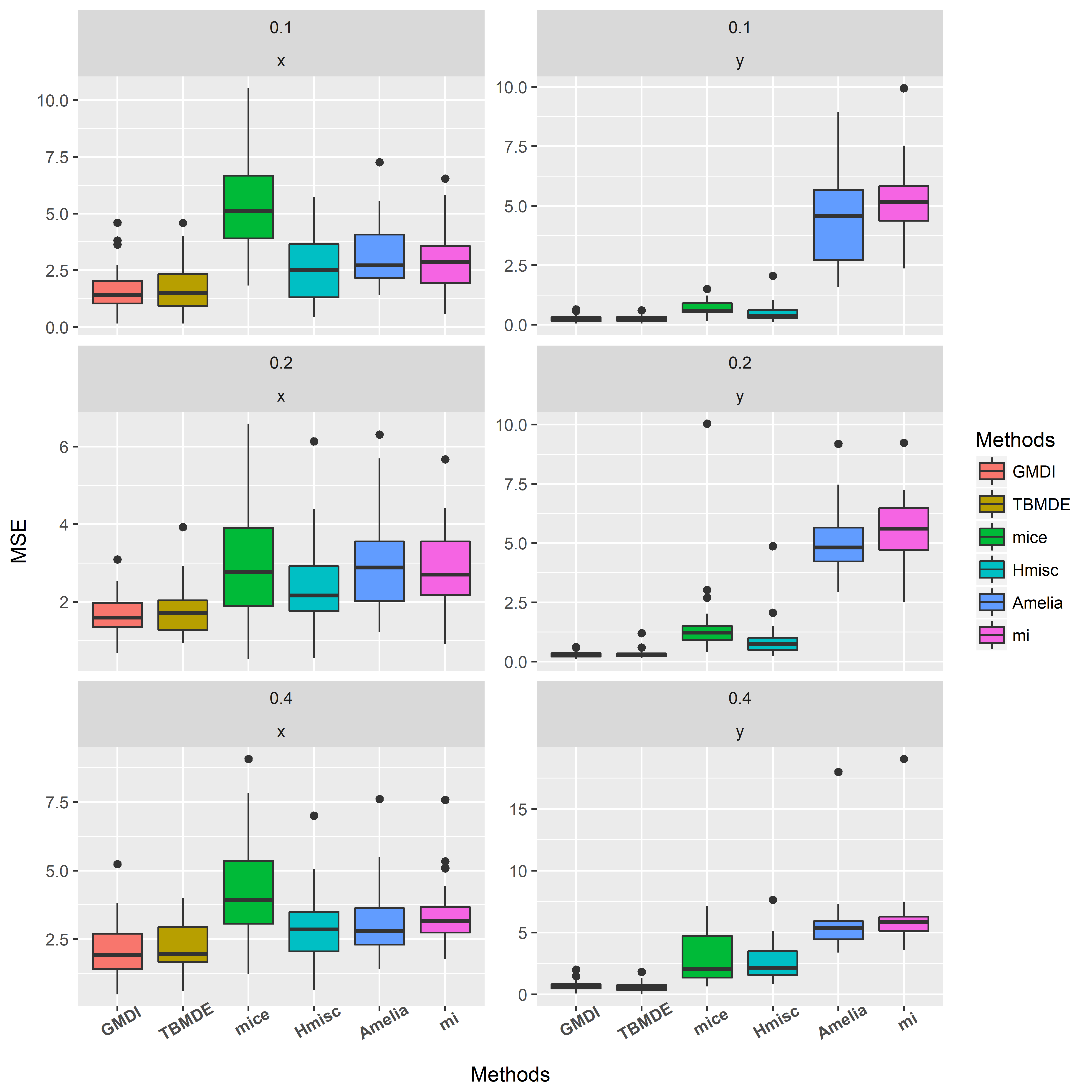
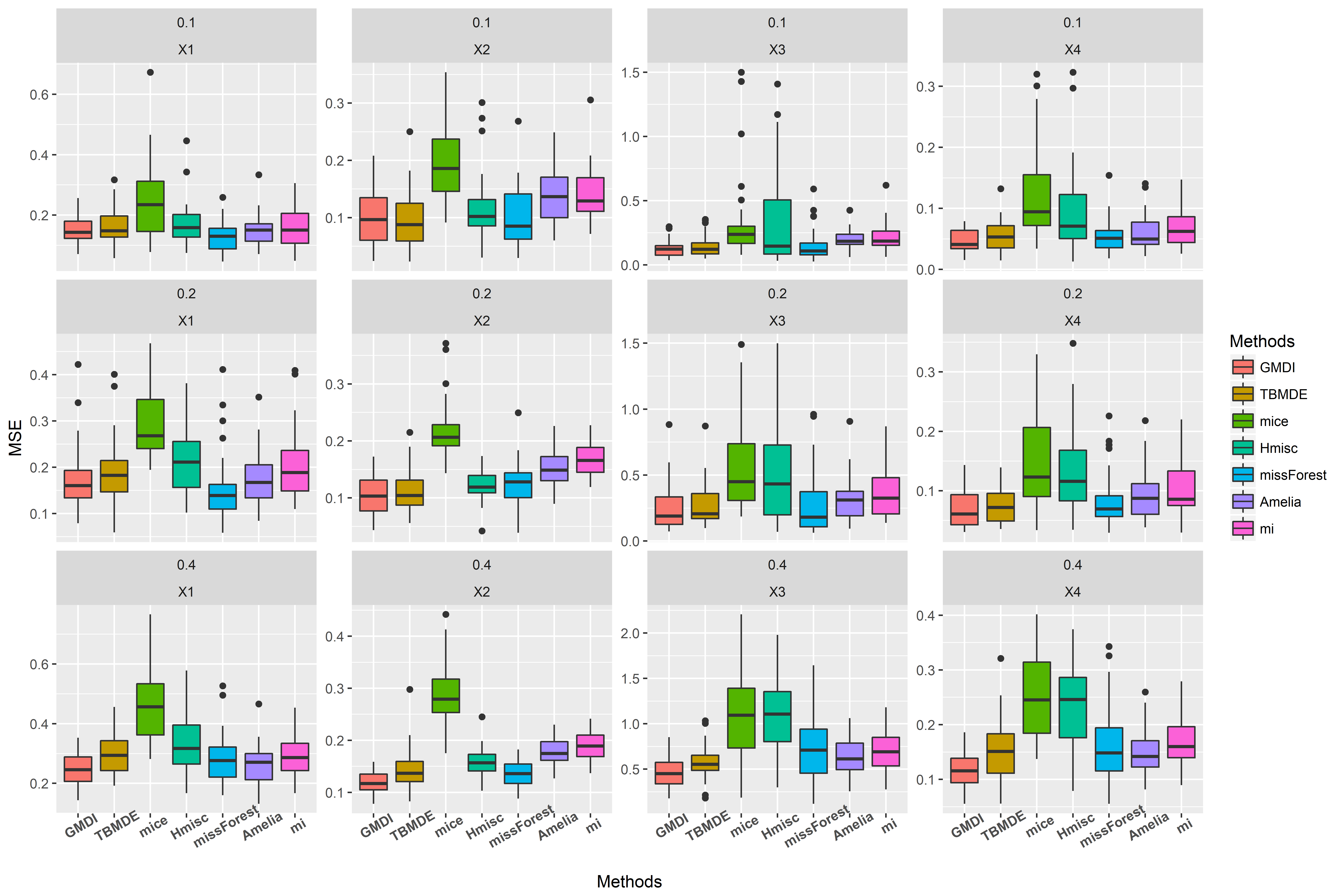
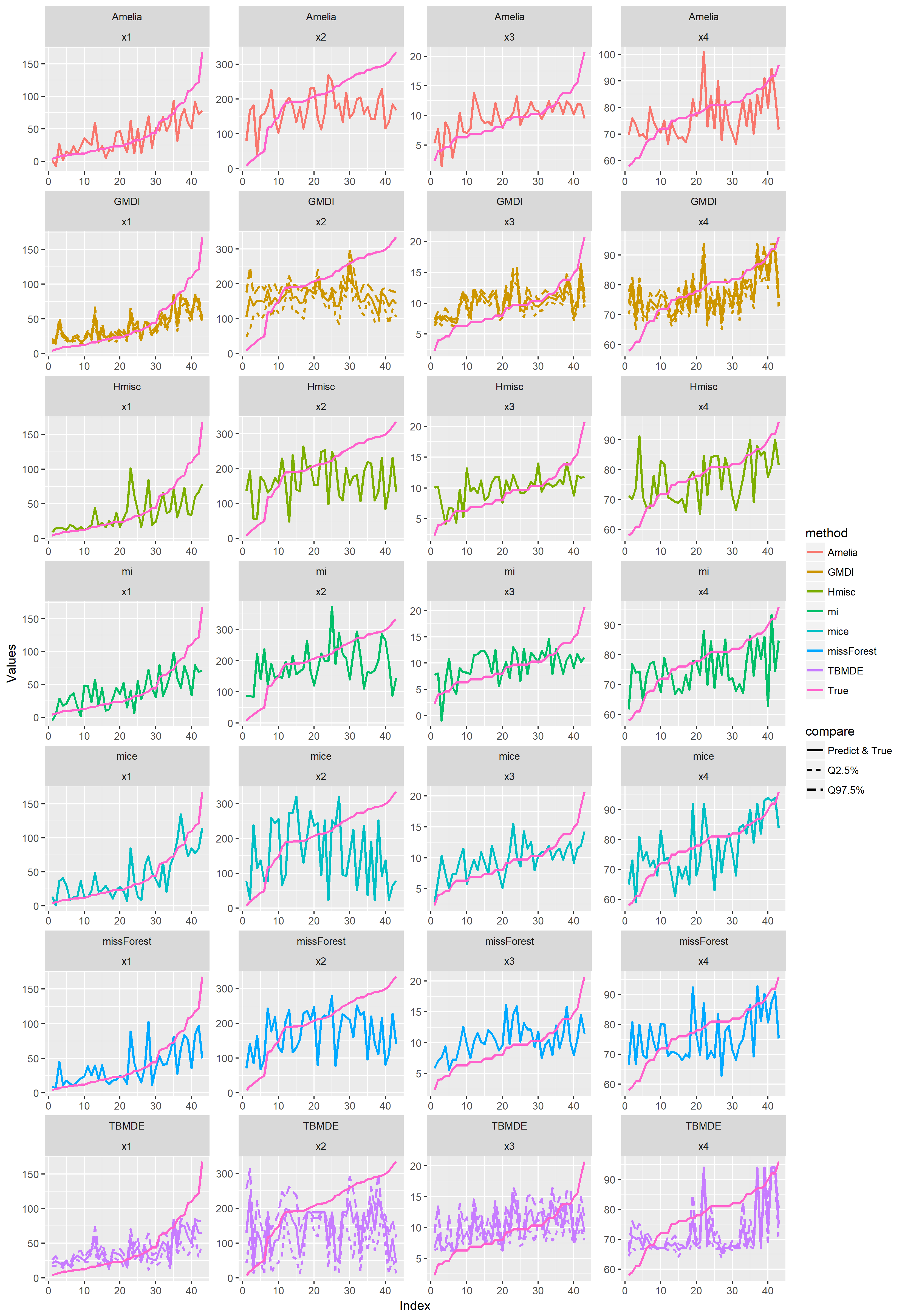
Since we don’t have prior information for the weights of knots, we set $\boldsymbol{\theta}\sim Dir(1/m,...,1/m)$ and $\lambda_{i}^{2}\sim InverseGamma(n_{i}^{0.4}+1,b_{i})$, where $n_{i}$ is the size of the observed data of the $i$th variable and $b_{i}$ is the sample variance of the $i$th variable, $i=1,...,p$. The motivation for the prior of $\lambda_{i}^{2}$ is that a rule-of-thumb estimator for the bandwidth $\lambda$ is approximately the standard deviation of the sample divided by the sample size to the one-fifth power and the mean of $InverseGamma(n_{i}^{0.4}+1,b_{i})$ is $b_{i}/n_{i}^{0.4}$ [12]. For the simulation data, we set the proportion of missing values for each variable $r\in\{0.1,0.2,0.4\}$ and the number of items in a data set $n=100$. For each $(r,n)$, we impute all the missing values in the data set using GMDI, TBMDE and four other imputation methods. (The random forest imputation method from R package “missForest" cannot be applied to two dimensional data.) As for TBMDE, we can only use the subset of the raw data where no missing value exists and we use (3) to estimate the missing values. Then we calculate the mean square error (MSE) between the missing values and the mean prediction values for each variable using the six methods. Especially for GMDI and TBMDE, we calculate the mean estimated marginal densities of $X$ and $Y$ with respect to sampled $(\boldsymbol{\theta},\boldsymbol{\lambda})$’s and use the Kolmogorov–Smirnov (KS) [14] method to test the goodness of fit. Figure 2 and Figure 3 display the MSE and p-values in the KS test,respectively, averaged over 30 simulation data sets. Figure 4 displays the estimated marginal densities for GMDI and TBMDE for a randomly generated data set. Figure 11 displays the true values and the predicted values in the six methods.

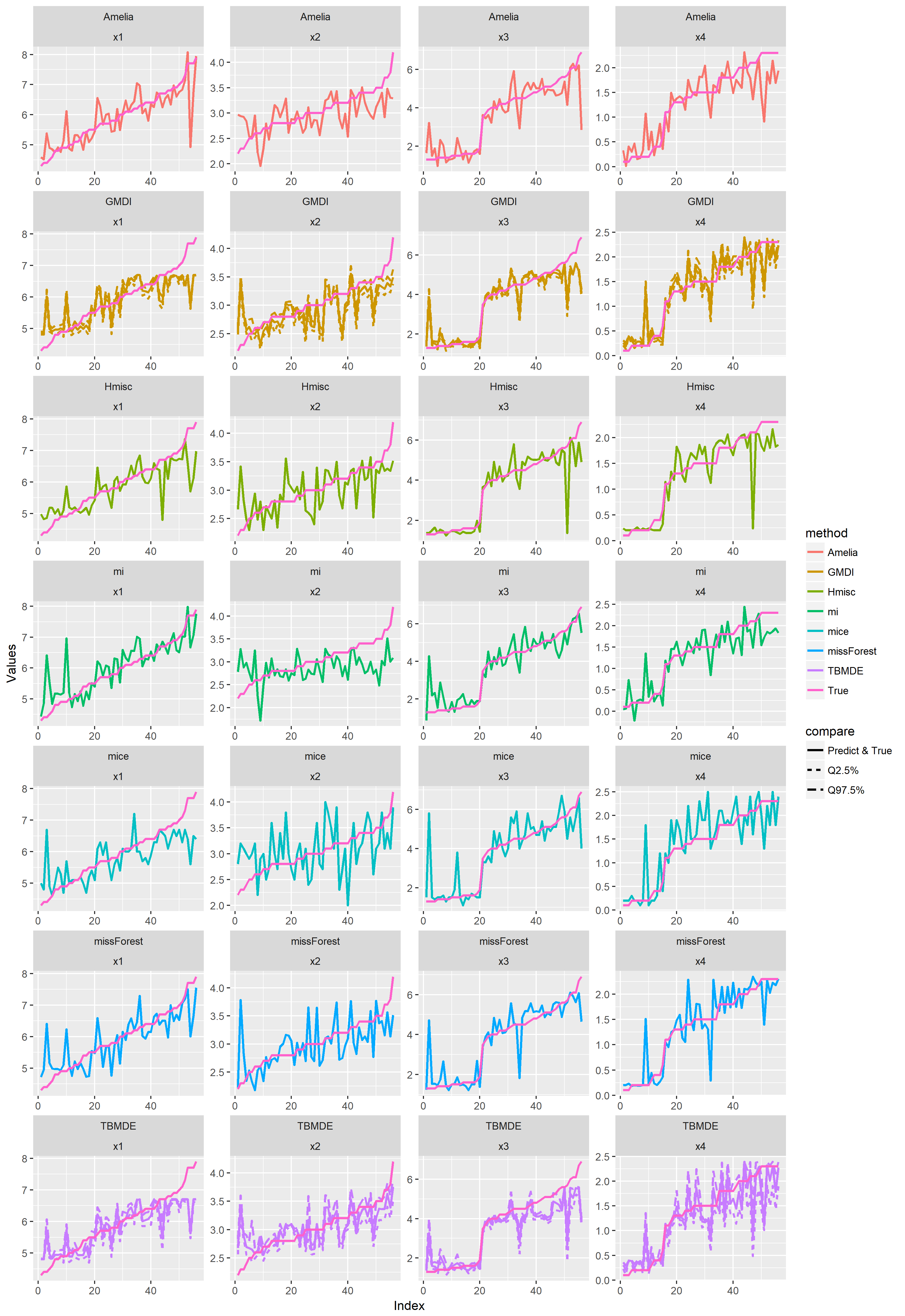
For the real data, the sample size of the raw data set is 111 for “airquality” and 150 for “Iris” and we set $r\in\{0.1,0.2,0.4\}$. Similar as before, we impute missing values, calculate the MSE and estimate the marginal densities of $X_{1},X_{2},X_{3},X_{4}$. The results of MSE are displayed in Figure 5, Figure 6 and the results of p-values in the KS test are displayed in Figure 7 and 8.

From Figure 2, 5 and 6, we see that the average MSE of GMDI is the smallest in many cases which shows its good performance in missing data imputation. Especially, in the four-dimensional cases, with the proportion of missing data $r$ increasing, the performance in missing data imputation of GMDI becomes better.

Figure 11, 12 and 13 show that the mean prediction values in GMDI and TBMDE are similar but GMDI has narrower empirical 95% credible intervals. Besides, the prediction values in GMDI and TBMDE are close to the true values, especially for the response variables ($y$ in Figure 4 and $x_{1}$ in Figure 12) and rather competitive among all the methods of missing data imputation.

From Figure 3, 7 and 6, we see that using the KS test, the average p-values in GMDI are larger than those in TBMDE in all cases which implies that the mean estimated joint density function in GMDI fits the data better than TBMDE. Moreover, when $n$ is fixed, with the proportion of missing data $r$ increasing, the average p-values in GMDI gradually dominate those in TBMDE. It shows that given a fixed $n$, the more missing data, the better GMDI is than TBMDE in density estimation. Figure 4, 9 and 10 show that the mean marginal densities estimated in GMDI fit the data better than TBMDE. Moreover, the empirical 95% credible intervals of the marginal densities in GMDI are narrower than those in TBMDE which implies the low variance of the density estimation in GMDI.

Furthermore, Table 2 displays the average computing time of GMDI and TBMDE for the real data set $airquality$. Since GMDI makes use of both the complete data and the observed variables of the missing data, the computing time of it is longer than that of TBMDE as expected. We can also see that the computing time of GMDI does not vary much as the proportion of missing values $r$ varies while the computing time of TBMDE does.

References

- [1] Ferguson, T.S. (1973), A Bayesian Analysis of Some Nonparametric Problems, The Annals of Statistics,1, 209-230. – (1983), Bayesian Density Estimation by Mixtures of Normal Distributions, in Recent Advances in Statistics, eds.H. Rizvi and J. Rustagi, New York:Academic Press, pp.287-302.
- [2] Escobar, M. D. & West, M. (1995). Bayesian Density Estimation and Inference using Mixtures. J. Am. Statist. Assoc. 90, 577-88.
- [3] Muller,P.,Erkanli, A.,West, M. Bayesian curve fitting using multivariate normal mixtures, Biometrika, Volume 83, Issue 1, 1 March 1996, Pages 67–79,
- [4] Little, R.J.A. (1988), Missing data adjustments in large surveys (with discussion), Journal of Business Economics and Statistics, 6, 287–301.
- [5] Stef van Buuren, Karin Groothuis-Oudshoorn (2011). mice: Multivariate Imputation by Chained Equations in R. Journal of Statistical Software, 45(3), 1-67. URL http://www.jstatsoft.org/v45/i03/.
- [6] Harrell, F.E. Jr. Package ‘HMISC’. (Updated June 4, 2010) cran.it.r-project.org/web/packages/Hmisc/Hmisc.pdf
- [7] Daniel J. Stekhoven (2013). missForest: Nonparametric Missing Value Imputation using Random Forest. R package version 1.4.
- [8] Honaker J, King G, Blackwell M., Amelia II: A program for missing data. Journal of Statistical Software. 2011;45:1-47.
- [9] Su Y-S, Gelman A, Hill J, Yajima M. Multiple imputation with diagnostics (mi) in R: opening windows into the black box. J Stat Softw 2011;45(2):1-31.
- [10] Van Buuren, S. (2012). Flexible Imputation of Missing Data. CRC/Chapman & Hall, Boca Raton, FL.
- [11] George Casella and Edward I. George (1992). Explaining the Gibbs Sampler. The American Statistician Vol. 46, No. 3 (Aug., 1992), pp. 167-174.
- [12] Silverman, B. W. (1986) Density Estimation, London: Chapman and Hall, pp. 48, (3.31).
- [13] Jun Shao(1991) Linear Model Selection by Cross-validation Journal of the American Statistical Association Volume 88, 1993 - Issue 422
- [14] Daniel, Wayne W. (1990). "Kolmogorov–Smirnov one-sample test". Applied Nonparametric Statistics (2nd ed.). Boston: PWS-Kent. pp. 319–330. ISBN 0-534-91976-6.
- [15] Horton P., Nakai K. (1996). A probabilistic classification system for predicting the cellular localization sites of proteins. In: Proceeding of the Fourth International Conference on Intelligent Systems for Molecular Biology 4: 109-115.
Appendix A
Appendix
If we do not consider prior on , we can use the following empirical procudure to choose bandwidth : is the bandwidth of variable . We implement a rule-of-thumb for choosing the bandwidth of a Gaussian kernel density estimator. It defaults to 0.9 times the minimum of the standard deviation and the interquartile range divided by 1.34 times the sample size to the negative one-fifth power (i.e. Silverman’s "rule of thumb", Silverman (1986))[12];
Appendix B Gibbs Sampler Review
Gibbs sampling [11] is a special case of the Metropolis–Hastings algorithm. The point of Gibbs sampling is that given a multivariate distribution it is simpler to sample from a conditional distribution than to marginalize by integrating over a joint distribution. Suppose we want to obtain samples of from a joint distribution . We denote the th sample of them as . We proceed as follows: we begin with some initial value and suppose denotes the conditional density of given . If we get the sample , we get the sample for each component of it under the mechanism
We repeat this step for times and we will get a renewed version of
If such sampling is performed, these important facts hold:
- 1.
The samples approximate the joint distribution of all variables.
- 2.
The marginal distribution of any subset of variables can be approximated by simply considering the samples for that subset of variables, ignoring the rest.
- 3.
The expected value of any variable can be approximated by averaging over all the samples.
Derivation of Algorithm 3:
where and are constants not related to .
The transition kernel density (TKD) of the Markov chain with respect to is
where , and , .
Then,
The last equality holds since the expression in the second to last line is symmetric with respect to and .
Hence,
which shows the density is stationary for the transition kernel density so the MCMC algorithm to sample given works.
Derivation of Algorithm 4:
where , and .