Confinement is one of the most fundamental properties of QCD. It can be viewed as a consequence of an approximately linear term in the QCD potential

between a quark and an antiquark in an overall colour singlet state, where $r$ is the distance between them and $\alpha_{\mathrm{s}}$ is the strong coupling constant. The presence of a linear term was first inferred from hadron spectroscopy (Regge trajectories), from which a $\kappa\approx 1$ GeV/fm can be extracted, and has later been confirmed by lattice QCD calculations.

The linear term dominates at large distances, and in the Lund string model only this term is used to describe the breakup of a high-mass ${\mathrm{q}}\overline{\mathrm{q}}$ system into several smaller-mass ones. Then the full colour field can be approximated by a one-dimensional string stretched straight between the ${\mathrm{q}}$ and $\overline{\mathrm{q}}$, Fig. 1. This string can be viewed as parametrizing the center of a cylindrical region of uniform width along its full length, such that the longitudinal and transverse degrees of freedom almost completely decouple.

The Lund model is easiest to understand in the context of a simple quark–antiquark pair created at the origin (e.g. by ${\mathrm{e}}^{+}{\mathrm{e}}^{-}$ annihilation) and moving out along the $\pm z$ axis. Neglecting the transverse degrees of freedom, the Hamiltonian can then be written as [11]

Here $|z_{{\mathrm{q}}}-z_{\overline{\mathrm{q}}}|$ is the distance between ${\mathrm{q}}$ and $\overline{\mathrm{q}}$, and $E_{{\mathrm{q}}}$ and $E_{\overline{\mathrm{q}}}$ are the energies of the ${\mathrm{q}}$ and $\overline{\mathrm{q}}$. With both assumed massless, it also holds that $E_{{\mathrm{q}}/\overline{\mathrm{q}}}=|\mathbf{p}_{{\mathrm{q}}/\overline{\mathrm{q}}}|=|p_{z,{\mathrm{q}}/\overline{\mathrm{q}}}|$.

From the Hamiltonian, the equation of motion gives rise to a linear relation between the space–time and the energy–momentum pictures

The signs of the derivatives depend both on the direction of motion of the parton and on the direction the string pulls it in. When the parton moves out along the $+z$ axis, e.g., the string pulls the parton in the $-z$ direction, and all signs are negative.

Next, more complicated string topologies need to be considered. An example is the ${\mathrm{Z}}^{0}$ decay into a pair of massless quarks, either of which can emit a gluon:

Both such radiation and the hadronization can occur over widely varying time scales in high-energy events, but in a local context the radiation takes place at time scales shorter than those of the hadronization itself. As a reasonable first approximation all three partons can thus be assumed created at the origin.

In the Lund model the colour flow is based on the limit of infinitely many colours [33]. Then there is one string piece from the ${\mathrm{q}}$ to the ${\mathrm{g}}$ and another from the ${\mathrm{g}}$ to the $\overline{\mathrm{q}}$, and the two do not interfere. The gluon thus can be viewed as a kink on a single string stretched from the ${\mathrm{q}}$ to the $\overline{\mathrm{q}}$.

The motion of the ${\mathrm{q}}{\mathrm{g}}\overline{\mathrm{q}}$ string system can conveniently be studied in a Lorentz frame where the ${\mathrm{q}}$ moves in the $+z$ direction, ${\mathrm{g}}$ in the $+x$ direction and $\overline{\mathrm{q}}$ in the $-z$ direction. Two string pieces are present initially, as illustrated in view 1 of Fig. 6. Each string piece defines a separate string region, which behaves similarly to the string piece of a ${\mathrm{q}}\overline{\mathrm{q}}$ system, except that it is now transversely boosted. The region formed by the ${\mathrm{q}}{\mathrm{g}}$ string evolves with time as

and correspondingly for $\overline{\mathrm{q}}{\mathrm{g}}$, but with $z\to-z$. Note the factor of 2 in the gluon four-momentum, which comes from the loss of energy–momentum to both string pieces attached to it. Unlike the simple ${\mathrm{q}}\overline{\mathrm{q}}$ system, the two string pieces are not at rest, but move in the transverse direction: the ${\mathrm{q}}{\mathrm{g}}$ string piece has a velocity vector $v_{x}=v_{z}=1/2$, while for the ${\mathrm{g}}\overline{\mathrm{q}}$ piece $v_{x}=-v_{z}=1/2$. The energy per unit string length is higher than for a string at transverse rest, but the lower string length drawn out per unit time exactly compensates, such that the force acting on the endpoints is of the same magnitude [27].

After time $t=E_{{\mathrm{g}}}(0)/2\kappa$ the gluon has lost all its energy and a new string piece is created by the inflowing momentum from the ${\mathrm{q}}$ and $\overline{\mathrm{q}}$, and is hence denoted as the ${\mathrm{q}}\overline{\mathrm{q}}$ region, see view 2. Later the ${\mathrm{q}}$ has also lost all its energy and starts to move in the $+x$ axis as it absorbs ${\mathrm{g}}$ four-momentum. The ${\mathrm{q}}$ eventually gains and re-emits half of the gluon energy, views 3 and 4. Subsequently it absorbs original $\overline{\mathrm{q}}$ four-momentum and moves in the $-z$ direction, views 5 and 6. A similar process occurs for $\overline{\mathrm{q}}$. As shown in view 7, the gluon will eventually reappear, and in view 8 the sequence starts to repeat, only with the momenta of ${\mathrm{q}}$ and $\overline{\mathrm{q}}$ swapped.

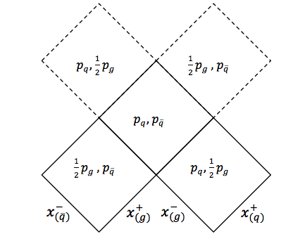
Although Fig. 6 is useful to visualize the time evolution of the system, the parameter plane picture is most convenient when addressing the kinematics [27]. This is a diagram that displays the different string regions in terms of the light-cone four-vectors defining each region, i.e. $p^{+}_{{\mathrm{q}}}=p_{{\mathrm{q}}}$, $p^{-}_{\overline{\mathrm{q}}}=p_{\overline{\mathrm{q}}}$ and $p^{+}_{{\mathrm{g}}}=p^{-}_{{\mathrm{g}}}=p_{{\mathrm{g}}}/2$ in the ${\mathrm{q}}{\mathrm{g}}\overline{\mathrm{q}}$ case, whose parameter plane is displayed in Fig. 7. The low regions represent the states in which none of the partons have lost their energy, corresponding to the two string regions in view 1 of Fig. 6, the ${\mathrm{q}}{\mathrm{g}}$ and the ${\mathrm{g}}\overline{\mathrm{q}}$ string pieces. The intermediate region corresponds to the new string piece created from the ${\mathrm{q}}$ and $\overline{\mathrm{q}}$ momenta once the gluon has lost all its energy. Finally, the upper regions are related to the two string pieces formed when ${\mathrm{g}}$ re-appears. Although the complete parameter plane picture (for half a period) is the one shown in Fig. 7, the dashed upper regions are normally neglected, since the system is assumed to fragment before then. This reasonable assumption avoids a large number of complications for handling fragmentation in these regions. The three remaining regions are then formed by the combination of one $+$ component and one $-$ one, where $\pm$ no longer relates to motion along the $\pm z$ axis, but more generically denotes the reference vector directed towards ($+$) or away from ($-$) the ${\mathrm{q}}$ end of the system.

From the parameter plane picture, the equations defining the hadron properties and the fragmentation process of section 2.2 can be easily generalized. For the ${\mathrm{q}}{\mathrm{g}}\overline{\mathrm{q}}$ system, the hadron momentum can generically be written as

The hadron mass enters via the constraint $p_{h}^{2}=m_{h}^{2}$. The other Lorentz invariant variable $\Gamma$ is obtained from the $\hat{x}^{\pm}$ fractions defined in section 2.2.2 as

The level lines of constant $m_{h}$ and constant $\Gamma$ again give hyperbolae inside each string region, where physically allowed, which connect at the borderline between regions. As before there will be (at most) one allowed solution to a given ($m_{h},\Gamma)$ pair, which can be found by starting in the current region and, if not found there, step by step move on to other possible regions. There are a number of complications that have to be overcome to do this [27].

The parameter-plane picture can be extended to a multiparton system, resulting in the most convenient approach to study the kinematics of any multiparton system. As an example, the parameter plane for a system consisting of three gluons, one quark and one antiquark is depicted in Fig. 8, where the turnover regions have been ignored. In such a system, there are four low regions, or initial regions, and six intermediate regions. The number of initial and intermediate regions can be generalized for any multiparton system formed by $n$ partons, out of which $n-2$ are gluons, as $n-1$ initial regions and $(n-1)(n-2)/2$ intermediate regions. The expression for the hadron four-momentum can also be generalized to an $n$-parton system by accounting for the momenta taken from each parton as

where usually most of the $x^{\pm}$ vanish. Apart from these aspects, the rest of the properties are similarly determined as in previous cases.

The fragmentation process in Pythia is based on the four-momenta of the partons created in the (semi)perturbative stages of the collision process, plus the partons in the beam remnants [34]. By the colour-connection between those partons, an LHC event is likely to contain several ${\mathrm{q}}{\mathrm{g}}_{1}{\mathrm{g}}_{2}\ldots{\mathrm{g}}_{n-2}\overline{\mathrm{q}}$ systems, that can be handled separately.

The production of each new hadron begins with the selection at random of whether to split it off from the ${\mathrm{q}}$ end or from the $\overline{\mathrm{q}}$ one of the system. The flavour of a new ${\mathrm{q}}\overline{\mathrm{q}}$ break of the string (where ${\mathrm{q}}$ may also represent an antidiquark), leads to the formation of a new hadron, as already described. Its mass is selected, according to a Breit–Wigner for short-lived particles with a non-negligible width. The transverse momentum is obtained as the vector sum of those of the hadron constituents, assuming that the old and new breakup vertices are in the same region. Then the longitudinal momentum fraction $z$ is picked according to the probability distribution in eq. (12), with the difference that the hadron mass has to be replaced by the transverse ditto, $m_{h}\to m_{\perp h}$. In a simple ${\mathrm{q}}\overline{\mathrm{q}}$ system, the new breakup vertex is easily obtained from the $(m_{\perp h},z)$ pair. Else the $\Gamma_{i}$ value of the new breakup is calculated using eq. (13), again with $m_{h}\to m_{\perp h}$, and a solution is sought to the $(m_{\perp h},\Gamma_{i})$ pair of equations. Vertex $i$ may end up in the same string region as $i-1$, or involve a search in other regions. Among technical complications of this search is that the transverse directions are local to each string region, which leads to discontinuities in the hyperbolae of constant $m_{\perp h}$ at the borders between string regions, that would not be there for $p_{\perp}=0$.

The random steps from both string ends continue until the remaining invariant mass of the system is deemed so small that only two final hadrons should be produced. Details on this final step can be found in Appendix A, along with the challenges encountered when implementing the space–time picture and the methods applied to solve them. Had the fragmentation always proceeded from the ${\mathrm{q}}$ end, say, the final step would always have been at the $\overline{\mathrm{q}}$ end, with the minor blemishes of this step concentrated there. Now these are instead smeared out over the whole event.

To begin, consider a breakup point $i$ in a simple ${\mathrm{q}}\overline{\mathrm{q}}$ system. Its location with respect to the origin of the energy–momentum picture, where ${\mathrm{q}}$ and $\overline{\mathrm{q}}$ have been created, is given by the $\hat{x}^{\pm}$ fractions. Then, considering $p^{+}$ to be the ${\mathrm{q}}$ four-momentum and $p^{-}$ the $\overline{\mathrm{q}}$ four-momentum, the location of breakup $i$ in the energy–momentum picture is defined as $\hat{x}_{i}^{+}p^{+}+\hat{x}_{i}^{-}p^{-}$. Recalling the linear relation between space–time and energy–momentum, eq. (3), the space–time location of breakup point $i$ thereby is defined as

Note that the ${\mathrm{q}}_{i}$ and $\overline{\mathrm{q}}_{i}$ generated by the string break are considered to be created in the same space–time vertex, even when quark masses and transverse momenta are included, such that ${\mathrm{q}}$ and $\overline{\mathrm{q}}$ have to tunnel some distance apart before becoming on-shell. Such effective vertices in practice is the best one can do.

Since hadrons are formed by two adjacent string breaks, the hadron production point should be related to these two. But the definition cannot be unique, since hadrons are composite and extended particles. For that reason, we propose three alternative definitions, illustrated in Fig. 9. Two breakup points, $i$ and $i+1$, with space–time coordinates $v_{i}$ and $v_{i+1}$, together define the ${\mathrm{q}}_{i}\overline{\mathrm{q}}_{i+1}$ subsystem that forms hadron $i$. One obvious choice is then to define the hadron production point as the average of the two,

red dot in the figure. Alternatively to this “middle” definition, the “late” hadron production point is where the two partons forming the hadron cross for the first time, green dot. Taking into account the hadron four-momentum $p_{h}$, the “late” hadron production point is offset from the “middle” definition as

Finally, an “early” definition, blue dot, is given by

which is where the backwards light cones of the $\overline{\mathrm{q}}_{i}$ and ${\mathrm{q}}_{i+1}$ vertices cross, just like the “late” definition is where the forwards light cones cross. In a causal world, this would be the latest time for information to be sent out that can correlate the breakup vertices to give the correct hadron mass. Note that the two endpoint hadrons are situated on the light cone with this “early” definition. The different results obtained with the three alternative definitions can be used as a measure of uncertainty, see section 4.1. If not stated otherwise, the choice in this article is the “middle” definition of eq. (24).

Multiparton systems are more complicated to address than a single ${\mathrm{q}}\overline{\mathrm{q}}$ string, as already demonstrated for the energy–momentum picture. Their complexity also affects the space–time implementation, which has to be extended to include several string regions. Initially consider a ${\mathrm{q}}{\mathrm{g}}\overline{\mathrm{q}}$ system formed by massless partons, with a parameter plane as in Fig. 10, ignoring the turnover regions. Since each string region separately behaves like a simple ${\mathrm{q}}\overline{\mathrm{q}}$ system, eq. (23) can be used. Nevertheless, the intermediate region is formed after the gluon has lost all of its energy, at a different location in space–time than the initial regions, so an offset has to be taken into account for it. From the linear relation between space–time and energy–momentum, the space–time offset for this region can be calculated as $v_{\mathrm{reg}}=p_{{\mathrm{g}}}/2\kappa$, where $p_{{\mathrm{g}}}$ is the four-momentum of the gluon. The factor of $1/2$ accounts for the fact that a gluon loses four-momentum twice as fast as a ${\mathrm{q}}$ or $\overline{\mathrm{q}}$, since it transfers four-momentum to two string pieces. Thus, the space–time location of a breakup located in the intermediate region is given by

If the system is composed of more than one gluon, also more than one intermediate region has to be taken into account, as illustrated in Fig. 11. In such cases, more gluons have to be included when determining the space–time offset of some intermediate regions, such as the ${\mathrm{q}}{\mathrm{g}}_{3}$ one. This region is created when both ${\mathrm{g}}_{1}$ and ${\mathrm{g}}_{2}$ have lost their energies, giving an offset $v_{\mathrm{reg}}=(p_{g_{1}}+p_{g_{2}})/2\kappa$.

A general expression for the space–time offset of any intermediate region in any multiparton system can be easily defined, if all partons are numbered consecutively, starting from the ${\mathrm{q}}$ end, and region labels $jk$ are for ones containing four-momenta from partons $j$ and $k,k\geq j$. The $jk$ region offset is found to be

where $p_{m}$ is the four-momentum of parton $m$, and for a breakup vertex in this region it thus holds that

While seemingly simple enough, there are a number of significant challenges to a robust implementation in a multiparton configuration, in part paralleling similar problems in the energy–momentum picture [27], in part going further. There are two main problems: the determination of the space–time location of the final breakup in the system, and the non-physical values of the $\hat{x}^{\pm}$ fractions that can arise when fragmentation moves to a new region. Those issues are further explained in appendices A and B, respectively, along with the solutions found to properly implement the space–time picture.

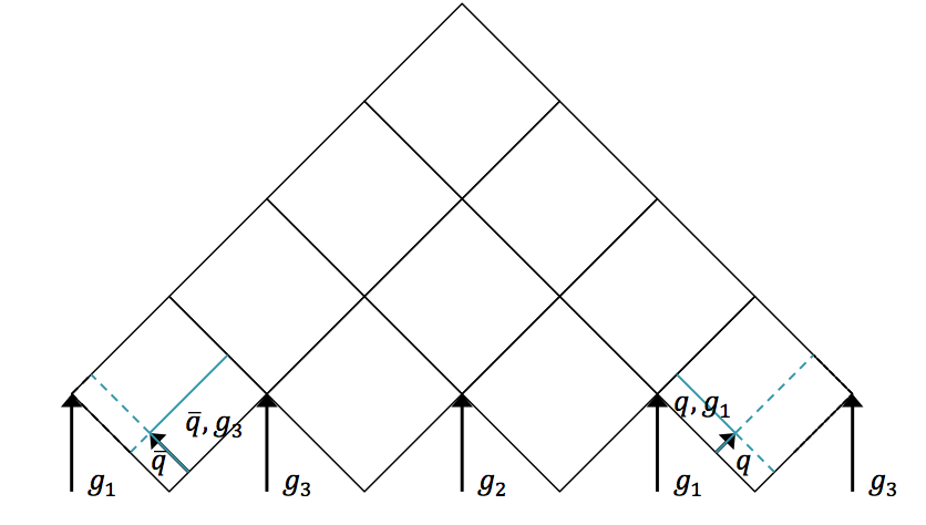
So far, gluons have only appeared in open strings between a ${\mathrm{q}}$ and a $\overline{\mathrm{q}}$ end, but it is also possible to have closed gluon loops, as exemplified in Fig. 12a for a ${\mathrm{g}}{\mathrm{g}}{\mathrm{g}}$ system. In order to reduce the problem to a familiar one, an initial ${\mathrm{q}}\overline{\mathrm{q}}$ is generated by string breaking in one of the string regions. This break should be representative of what ordinary fragmentation is expected to give. Thus the region is chosen at random, but with a bias towards ones with larger masses, where more ordinary string breaks are to be expected. Inside that region, the $\Gamma$ value of the vertex is chosen according to eq. (14), and a further random choice gives the longitudinal location of the breakup. Having taken this step, the $n$-gluon-loop topology is effectively mapped onto an $(n+1)$-parton open string with ${\mathrm{q}}$ and $\overline{\mathrm{q}}$ as endpoints. The key difference is that, unlike open strings considered so far, $\Gamma_{{\mathrm{q}}}=\Gamma_{\overline{\mathrm{q}}}\neq 0$.

As an example, the parameter plane for a gluon-loop consisting of three gluons is displayed in Fig. 12b. In this case, the string between ${\mathrm{g}}_{1}$ and ${\mathrm{g}}_{3}$ has broken into two string pieces, generating two new string regions, ${\mathrm{g}}_{1}{\mathrm{q}}$ and ${\mathrm{g}}_{3}\overline{\mathrm{q}}$. Although the full ${\mathrm{g}}_{1}{\mathrm{g}}_{3}$ region is duplicated in the parameter plane, in the right endpoint region only the “active area” between ${\mathrm{q}}$ and ${\mathrm{g}}_{1}$ is open to fragmentation, while the left endpoint region only uses the complementary area between ${\mathrm{g}}_{3}$ and $\overline{\mathrm{q}}$. Apart from that, the fragmentation process can now play out in the same way as for an open string, with the same rules for the space–time locations of the breakups. Note that the ${\mathrm{q}}$ and $\overline{\mathrm{q}}$ “endpoints” correctly will be assigned the same creation vertex in this procedure.

Strings can be viewed as the center of cylindrical tubelike regions of directed colour flow. So far we have assigned production vertices as if they all were in the very center of the string. A more realistic picture is to introduce some transverse smearing. For simplicity this is done according to a two-dimensional Gaussian

where $x$ and $y$ are transverse spatial coordinates and $\sigma$ is the width of the distribution.

The width of the string should be of typical hadronic scales, but related to confinement in two dimensions rather than three. Taking the proton radius $r_{{\mathrm{p}}}\approx 0.87$ fm [35] as starting point, the default $\sigma=r_{{\mathrm{p}}}/\sqrt{3}$ then gives a

The smearing in transverse space might generate unwanted situations, such as negative values for the $\Gamma$ parameter of the breakup points. Since the space–time location is first obtained from the fragmentation picture in the longitudinal direction, the squared invariant time should not change when introducing smearing. Therefore, the time coordinate is adjusted after including the smearing in transverse space, in order to retain the $\Gamma$ value determined by the longitudinal scheme. Alternative procedures could be envisioned, in particular when the collision process itself does not happen in the origin, but for now this smearing possibility is good enough to indicate trends.

As illustrated in section 2.2.5, the origin of the massive and massless oscillations are displaced for technical reasons; correspondingly the initial point of the massive oscillation is offset from the origin of the space–time coordinate system. Since the fragmentation process is performed in the massless system, the space–time locations of the breakups have to be adjusted.

To determine the offset, consider the ${\mathrm{q}}\overline{\mathrm{q}}$ system in Fig. 13a, studied in the CM frame, with ${\mathrm{q}}/\overline{\mathrm{q}}$ moving in the $\pm z$ directions. In this case the ${\mathrm{q}}$ and $\overline{\mathrm{q}}$ masses are different, with $m_{{\mathrm{q}}}>m_{\overline{\mathrm{q}}}$. At time $t=0$ we have $p_{0}=p_{z,{\mathrm{q}}}=-p_{z,\overline{\mathrm{q}}}$ and $E_{\mathrm{cm}}=E_{{\mathrm{q}}}+E_{\overline{\mathrm{q}}}$, with $p_{0}$, $E_{{\mathrm{q}}}$ and $E_{\overline{\mathrm{q}}}$ given by standard two-body decay kinematics. The massive oscillation in Fig. 13a is offset both in time and $z$-component of space, represented as $\Delta t$ and $\Delta z$. The former can be determined from the difference between the time coordinates at which the massless and massive quarks lose their three–momenta, $t_{\mathrm{massless}}$ and $t_{\mathrm{massive}}$ in Fig. 13a, i.e. 

The process to define the space offset is slightly different. In Fig. 13a, the distance of the massive ${\mathrm{q}}$ endpoint to the centre of the massive oscillation is denoted $z_{1}$, while $z_{2}$ is the distance of the massive ${\mathrm{q}}$ endpoint to the centre of the massless system. The equation of motion then gives

The time and space offsets can be combined as

where $p_{0{\mathrm{q}}}$ and $p_{0\overline{\mathrm{q}}}$ are the four-vectors of the equivalent massless system, cf. eq. (18). Hence, for each vertex in a region formed by at least one massive quark, the space–time location is defined as usual from the massless system, $v_{\mathrm{massless}}$, and then corrected to

For more complex topologies, such as multiparton systems consisting of a massive ${\mathrm{q}}$ and/or $\overline{\mathrm{q}}$ and several gluons, the effect of the massive ${\mathrm{q}}$ or $\overline{\mathrm{q}}$ is only non-negligible in the lowest respective endpoint region. Therefore, the massive correction is only performed in those regions.

Also the space–time location of the massive endpoint quark “vertex” has to be offset, away from what it would have been for a massless quark. This is exemplified in Fig. 13b, for the same massive ${\mathrm{q}}\overline{\mathrm{q}}$ system as before. The three vertices $v_{1}$, $v_{{\mathrm{q}}}$ and $v_{2}$ correspond to the space–time location of the massless endpoint, the massive turning point and the closest breakup to the massless endpoint, respectively. The system can be studied in a Lorentz frame where the three vertices are simultaneous, $v_{1,t}=v_{2,t}=v_{{\mathrm{q}},t}$. Then, linearity between energy–momentum and space–time gives

where $m_{{\mathrm{q}}}$ is the mass of the heavy quark and $m_{h}$ the mass of the hadron formed from the vertices $v_{1}$ and $v_{2}$. From this $v_{z,{\mathrm{q}}}$ can be extracted. Recast in Lorentz-invariant four-vector notation, this gives

Note that, after the correct endpoint location has been determined, the offset correction of eq. (35) has to be included. If a system is formed by a massless ${\mathrm{q}}$ and a massive $\overline{\mathrm{q}}$, say, eq. (37) has to be applied only to the massive $\overline{\mathrm{q}}$, while the offset in eq. (35) has to be used both for ${\mathrm{q}}$ and $\overline{\mathrm{q}}$.

A final feature is that the oscillation period for a hadron composed of massive quarks is shorter than a same-mass one with massless quarks. This discrepancy only affects the estimation of the “late”, $v_{l}^{h}$, and “early”, $v_{e}^{h}$, definitions of hadron production points. The expression in eq. (25) and eq.( 26) now become

where $\alpha_{\mathrm{red}}$ accounts for the reduced oscillation period. This parameter is determined in the hadron rest frame by the absolute three-momentum of the quarks forming the hadron

where $m_{h}$ is the mass of the hadron and $m_{{\mathrm{q}}}$ and $m_{\overline{\mathrm{q}}}$ the masses of the constituent ${\mathrm{q}}$ and $\overline{\mathrm{q}}$, respectively. Needless to say, these semiclassical estimates of oscillation periods cannot be taken too literally. It could be argued that all hadrons, light as heavy, have hadronic sizes of order 1 fm, and should have essentially common oscillation periods related to that. That would give us problems notably for pions, however, which are abnormally light in relation to their size.

Up until now, only open ${\mathrm{q}}{\mathrm{g}}_{1}{\mathrm{g}}_{2}\ldots{\mathrm{g}}_{n-2}\overline{\mathrm{q}}$ and closed ${\mathrm{g}}_{1}{\mathrm{g}}_{2}\ldots{\mathrm{g}}_{n}$ strings have been considered. A third possibility is junction topologies, wherein three string pieces meet in a common vertex [36], and whereby the junction effectively carries the baryon number of the system. Such topologies can arise e.g. when the three valence quarks are all kicked out of an incoming proton, but there are also scenarios in which further junctions and antijunctions may be formed [37].

A junction system consists of three different “legs”, each stretched from an endpoint quark via a number of gluons in to the junction. In Pythia the fragmentation process is most conveniently defined in the rest frame of the junction. Here the total energy of each leg is determined, and the two legs with the lowest energies are fragmented from the respective ${\mathrm{q}}$ end inwards. The process stops when the next step would require more energy than left in the leg. Once the two initial legs have fragmented, the two leftover ${\mathrm{q}}$ from the respective last breaks are combined to create a diquark. Together with the third leg and its original endpoint ${\mathrm{q}}$, this diquark defines a final string system, which now fragments as a normal open string.

The assignment of space–time locations in junction topologies introduces no new principles, but requires some extra bookkeeping. The three junction legs are considered as three different systems, to be dealt with in the same order as they fragmented, starting from the leg with the lowest energy.

Low-invariant-mass systems hadronize about as high-mass ones, even if kinematics is more constrained. The exception is when the invariant mass of the system is so low that only one hadron can be formed. In such cases, the “early” hadron production point is at the origin of the ${\mathrm{q}}\overline{\mathrm{q}}$ system, i.e. $v_{e}^{h}=(0;0,0,0)$. Note that smearing in transverse space will give rise to negative squared invariant times in such cases. This is not a problem if the reason is that the collision of two Lorentz-contracted proton “pancakes” naturally would lead to a spread of $x,y$ coordinates of collisions at $t=0$. The “middle” and “late” definitions are calculated from the four-momentum $p_{h}$ of the hadron as $v^{h}=p_{h}/2\kappa$ and $v_{l}^{h}=p_{h}/\kappa$, respectively.

Finally, many of the hadrons produced during the string fragmentation are unstable and decay further, a process known as secondary particle production. In such cases the invariant lifetime is selected at random according to an exponential decay, $P(\tau)\propto\exp(-\tau/\langle\tau\rangle)$, where $\langle\tau\rangle$ is the tabulated average lifetime [35]. For short-lived particles it is rather the width $\Gamma$ of the mass distribution that is known, and then one can use $\langle\tau\rangle=\hbar c/\Gamma$. Given a known hadron production vertex, the decay one becomes

for a hadron with four-momentum $p_{h}$ and mass $m_{h}$. This equation can be used recursively through decay chains, also e.g. for leptons.

Truly stable particles are only ${\mathrm{e}}^{\pm}$, ${\mathrm{p}}$, $\overline{\mathrm{p}}$, $\gamma$ and the neutrinos. Also some weakly decaying particles with long lifetimes are effectively treated as stable by default: $\mu^{\pm}$, $\pi^{\pm}$, ${\mathrm{K}}^{\pm}$, ${\mathrm{K}}_{L}^{0}$ and ${\mathrm{n}}/\overline{\mathrm{n}}$.

In this article we only address the space–time picture of hadronization. In the context of a hard collision process, say ${\mathrm{q}}{\mathrm{g}}\to{\mathrm{q}}{\mathrm{g}}$, also perturbative emission of further partons off the two scattered partons is extended in space and time. This is related to the regeneration time of the QCD field, mainly consisting of gluons, at typical time scales of order

for emitted partons of energy $E$ and transverse momentum $p_{\perp}$ [38]. This expression is conveniently split into a “Heisenberg uncertainty” factor ($p_{\perp}$ is a measure of the off-shellness of intermediate propagators) and a “time dilation” factor, as indicated. Similar relations hold for emissions off the two incoming partons.

Typically, parton shower descriptions in event generators such as Pythia stop at scales of the order ${\mathrm{p}}_{\perp\mathrm{min}}=0.5-1$ GeV, mainly because $\alpha_{\mathrm{s}}$ becomes so big that perturbation theory cannot be trusted below that. (The current default value for Pythia final-state radiation is 0.5 GeV, but that is the $p_{\perp}$ for each daughter of a branching with respect to the mother direction, meaning a separation of 1 GeV between the two daughters. eq. (41) should not be trusted up to factors of 2 anyway.) This corresponds to a $\tau_{\mathrm{regen}}\approx 0.25$ fm, say, to be compared with the average hadronization time $\langle\tau_{\mathrm{had}}\rangle\approx 1.3$ fm (see section 4.2 below), i.e. about a factor five difference. To a good first approximation, the simulated perturbative activity can therefore be viewed as happening in a single point as far as the hadronization process is concerned. This is even more so for the hard perturbative activity that gives rise to separate jets, for which $p_{\perp}\gg 1$ GeV. The emissions that possibly are simulated below 1 GeV can only give small wrinkles on the strings stretched between the main partons.

The comparison of invariant time generalizes to hold everywhere in an event, since time dilation works the same way for showers and hadronization. That is, a perturbative splitting at high energy and low $p_{\perp}$ may occur at large time scales as measured in the rest frame of the event, when hadronization already started in the central region, but still well before it will begin in the part of the event that could be affected by the splitting.

At the end of the Pythia showers, the total number of partons in a typical LHC event is roughly half of the number of primary hadrons later produced. Given that the size, in each of three spatial dimensions, is only a fifth for the partonic system compared with the hadronic one, it might seem that the partonic density is much higher than the the hadronic one, and that partonic close-packing would be a more severe issue than hadronic ditto. Partons don’t have a well-defined size, however. A newly created parton could be assigned a vanishingly small size, and then the colour field surrounding it would expand with the speed of light. Thus the partonic size could be equated with the time since creation, multiplied by a standard time dilation factor.

At early times the partonic system of a collision therefore expands in size at about the same rate as the size of partons, and any net effect comes from the rise of the total number of partons as the cascade evolves from early times. Here the colour coherence phenomenon enters, however [38]. It is the obervation that the two daughters of a ${\mathrm{q}}\to{\mathrm{q}}{\mathrm{g}}$ or ${\mathrm{g}}\to{\mathrm{g}}{\mathrm{g}}$ branching share a newly-created colour-anticolour pair, that cannot contribute to the radiation until the partons are more separated than the wavelength of the further radiated partons. This gives a mechanism for close-packing avoidance, in event generators implemented in terms of angular or $p_{\perp}$ ordering of radiation.

Had the parton shower been allowed to evolve further than the current cutoff, the partonic multiplicity and the partonic overlap would have increased as the $\Lambda_{\mathrm{QCD}}$ scale of $\approx 0.3$ GeV is approached. By then the naive size of partons would be of the order of 0.7 fm, which is about the expected transverse size of strings, and soft partons emitted at this stage form part of the emergent strings. We don’t know how to model these late stages of the cascade, but any effects coming from them are included in the tuned parameters of the string fragmentation framework.

The picture painted here is based on studying one partonic cascade. Since protons are composite object, however, several partonic subcollisions can occur when two protons collide — MPIs. One therefore also should worry about the overlap of cascades from different MPIs — partonic rescattering. In part this issue has been studied [39], and shown to give small effects. That study only included the effects of parton multiplication by initial-state radiation, as encoded in parton distribution functions, and thus did not address the effects of collisions between partons from two separate MPI subcollisions. In general, however, MPIs occur at different transverse locations when the two Lorentz-contracted protons collide, and the products move out in different rapidities and azimuthal directions. Also here it is therefore plausible with only minor overlap at early times and large perturbative scales. (In a relative sense; most MPIs do not have all that large $p_{\perp}$ values.) The overlap becomes relevant at later scales, where colour reconnection is the currently favoured mechanism for interactions between the emerging colour fields.

Another issue that we would like to comment on is the folklore that “fast particles are produced early”. This would seem to be in contradiction with the string picture, where hadronization begins with slow particles in the central region and then spreads outwards to faster particles at later times, roughly along a hyperbola of constant invariant time. But it is all a matter of what comparison one has in mind, and what production time definition is used [40]. Consider the “first” (“leading”) hadron, i.e. the one closest to the quark end of a ${\mathrm{q}}\overline{\mathrm{q}}$ string. For it $\Gamma_{i-1}=\Gamma_{0}=0$, such that eq. (13) and eq. (9) together give

The faster the hadron, the earlier the string break in invariant time: $\Gamma_{1}\to 0$ for $z_{1}\to 1$. Also the time in the string rest frame,

with $E_{{\mathrm{q}}}$ the quark energy, is decreasing for increasing $z_{1}$.

This reasoning generalizes: an event with few, fast particles can only be obtained when the $\Gamma$ values and the breakup times are small. Conversely, events with high multiplicities of lower-momentum hadrons require high $\Gamma$ values and late hadronization times. Whether early or late invariant times, however, the hadronization will still start in the middle and spread outwards.

Three definitions of hadron production points were presented in section 3.1, to allow estimates of the uncertainty in the description. Here the three resulting longitudinal and transverse space–time distributions are compared. For the former $y_{\tau}$ is introduced as a space–time correspondent to ordinary rapidity $y$:

while the latter is shown as a function of $r=\sqrt{x^{2}+y^{2}}$. Note that the longitudinal variable is dimensionless while the transverse one is expressed in units of fermi (fm). Although formally unrelated, the dynamics of string fragmentation introduces a strong correlation between $y$ and $y_{\tau}$, as illustrated in Fig. 14 for the default “middle” definition of production points. The spread from the diagonal comes from a number of effects, such as the probabilistic fragmentation process, given by eq. (12), and hadronic decays.

Figs. 15 and 16 display the longitudinal and transverse spectra for ${\mathrm{p}}{\mathrm{p}}$ collisions at $\sqrt{s}=13$ TeV given by the “early”, “middle” and “late” definitions of hadron production points, represented in green, red and blue, respectively. In the same figures, the spectra for a single string, at the same CM energy, using the “middle” definition are also illustrated in black. Both primary and secondary hadrons are taken into account.

The longitudinal spectra for the different definitions are very similar, as can be seen in Fig. 15. The largest disagreement is visible around $y_{\tau}\approx 0$, where the spectra of the “early” definition peaks more, but “early” also has more particles at the very largest $y_{\tau}$ values. In short, the “early” alternative maximizes the extreme behaviour of hadron production, whereas the “late” one minimizes it. The differences are not bigger than that we can consider the “middle” definition a fairly reliable one.

Similar conclusions are drawn from the transverse spectra, shown in Fig. 16. The spectrum for ${\mathrm{q}}\overline{\mathrm{q}}$ events is a consequence of the transverse smearing, section 3.4, and of particle decays; otherwise primary production would all be at $r=0$. In contrast, ${\mathrm{p}}{\mathrm{p}}$ events are constructed out of a large number of strings stretched between the partons from hard collisions, parton showers and beam remnants, all of them intrinsically with a transverse motion. Therefore the smearing is important for the spectrum at low $r$ values, as can be seen in the difference between the two “middle” $r$ distributions, while the distribution at larger $r$ values is rather insensitive. The difference between the “early”, “middle” and “late” production points is larger than for the longitudinal spectra, but still sufficiently close as to give confidence that meaningful results can be obtained. In the following, all plots will be for the “middle” definition.

The number of hadrons is shown as a function of time for a single string with $\sqrt{s}=20$ GeV in Fig. 17. The red curve corresponds to the number of primary hadrons, formed by the string fragmentation, that have not decayed at the time, while the green curve represents the number of secondary hadrons, from particle decays. The total number of hadrons, illustrated in blue, is the sum of primary and secondary hadrons. The brown curve represents the number of final (i.e. stable) hadrons, see section 3.6. Finally, the black curve depicts the number of hadrons with $|z|<0.5$ fm, to be discussed in section 4.3.

For the $20$ GeV simple ${\mathrm{q}}\overline{\mathrm{q}}$ system in its rest frame, the string can at most extend 10 fm in the $\pm z$ direction (for $\kappa=1$ GeV/fm). This happens at $t=10$ fm, since the massless quarks move with the speed of light. The primary hadron production therefore must stop at this time, as visible in Fig. 17. Decays make the number of hadrons continue to rise also beyond this time, but only slowly. Actually many hadrons, like the $\rho^{\pm,0}$ ones, are so short-lived that they decay within some fm of having been produced.

Note that there are almost no hadrons in the system up until $t\approx 0.5$ fm, since the string has to have time to begin stretching out before it can begin to fragment. This is further illustrated in Fig. 18, with the invariant time distribution of primary hadron production points in the ${\mathrm{q}}\overline{\mathrm{q}}$ system. By default, the parameters $a$ and $b$ in eqs. (12) and (14) are set to $a=0.68$ and $b=0.98$ GeV^-2 [41], giving rise to a suppression of small $\Gamma$ values of breakup vertices, and thereby also of small hadron production times. In detail, the relation between $\Gamma$ and $\tau$, eq. (9), implies $P(\Gamma)\propto\Gamma^{a}{\mathrm{d}}\Gamma\propto\tau^{2a}\,\tau\,{\mathrm{d}}\tau=\tau^{2a+1}\,{\mathrm{d}}\tau$ for $\tau\rightarrow 0$. Furthermore, the expectation value of $\langle\Gamma\rangle=(1+a)/b\approx 1.7$ GeV² gives $\langle\tau\rangle\approx\sqrt{\langle\Gamma\rangle}/\kappa\approx 1.3$ fm, in agreement with Fig. 18. Because those aspects are typical of the fragmentation process, a similar behaviour is also observed in ${\mathrm{p}}{\mathrm{p}}$ collisions.

The time evolution of hadron production in 13 TeV ${\mathrm{p}}{\mathrm{p}}$ events is shown in Fig. 19 for $t\leq 20$ fm. Although the qualitative behaviour is similar to the one in ${\mathrm{q}}\overline{\mathrm{q}}$ systems, the temporal evolution is smoother and the number of hadrons generated per unit time increases more rapidly in the ${\mathrm{p}}{\mathrm{p}}$ case. These effects are direct consequences of the presence of several string systems in ${\mathrm{p}}{\mathrm{p}}$ events, possibly extending all the way out to 6500 fm from the origin.

Fig. 20 extends the ${\mathrm{p}}{\mathrm{p}}$ description up to $10^{15}$ fm $=1$ m. As in the case of the ${\mathrm{q}}\overline{\mathrm{q}}$ system, the total number of primary hadrons increases until fragmentation is over, which now is at $t\approx 10^{3}$ fm owing to the higher energy. Decays deplete the number of remaining primary hadrons but increase the number of secondary ones. The significant drop in the number of hadrons at $t\approx 10^{8}$ fm is from electromagnetic decays of the $\pi^{0}$, mainly $\pi^{0}\to\gamma\gamma$. Although the lifetimes of ${\mathrm{s}}$, ${\mathrm{c}}$ and ${\mathrm{b}}$ hadrons typically are at the mm to cm scales (more long-lived ones, like ${\mathrm{K}}^{\pm}$, being considered stable here), their decays are still ongoing at 1 m, owing to time dilation of the frequently fast-moving hadrons.

Most of the expansion of the system is along the $z$ axis, i.e. the $|z|$ distribution of hadron production would look similar to the $t$ one in Fig. 20, except for the lack of a suppression at $z=0$. It is therefore interesting to show the radial evolution separately, Fig. 21, for the same $t$ range. Overall the two figures resemble each other, but all the relevant features have been compressed owing to the lower radial velocities. The $\pi^{0}\to\gamma\gamma$ decay is shifted from $t\approx 10^{8}$ fm to $r\approx 10^{6}$ fm, for instance. The impact of weak ${\mathrm{s}}$, ${\mathrm{c}}$ and ${\mathrm{b}}$ hadron decays are better visible in the range between 1 and 100 mm; beyond that scale essentially all relevant decays have already occurred. At the other end of the scale, note that around half of the hadron production occurs in $r<1$ fm; there is no equivalent dynamical suppression of small $r$ as there is of small $t$.

References

- [1] J. Campbell, J. Huston and F. Krauss, “The Black Book of Quantum Chromodynamics : A Primer for the LHC Era,” Oxford University Press (2017), ISBN: 9780199652747
- [2] T. Sjöstrand and M. van Zijl, Phys. Rev. D 36 (1987) 2019. doi:10.1103/PhysRevD.36.2019
- [3] T. Sjöstrand, Adv.Ser.Direct.High Energy Phys. 29 (2018) 191 [arXiv:1706.02166 [hep-ph]].
- [4] S. Schael et al. [ALEPH and DELPHI and L3 and OPAL and LEP Electroweak Collaborations], Phys. Rept. 532 (2013) 119 doi:10.1016/j.physrep.2013.07.004 [arXiv:1302.3415 [hep-ex]].
- [5] A. Buckley et al., Phys. Rept. 504 (2011) 145 doi:10.1016/j.physrep.2011.03.005 [arXiv:1101.2599 [hep-ph]].
- [6] T. Sjöstrand, S. Mrenna and P. Z. Skands, JHEP 0605 (2006) 026 doi:10.1088/1126-6708/2006/05/026 [hep-ph/0603175].
- [7] T. Sjöstrand, S. Ask, J. R. Christiansen, R. Corke, N. Desai, P. Ilten, S. Mrenna and S. Prestel et al., Comput. Phys. Commun. 191 (2015) 159 [arXiv:1410.3012 [hep-ph]].
- [8] M. Bähr et al., Eur. Phys. J. C 58 (2008) 639 doi:10.1140/epjc/s10052-008-0798-9 [arXiv:0803.0883 [hep-ph]].
- [9] J. Bellm et al., Eur. Phys. J. C 76 (2016) no.4, 196 doi:10.1140/epjc/s10052-016-4018-8 [arXiv:1512.01178 [hep-ph]].
- [10] T. Gleisberg, S. Höche, F. Krauss, M. Schönherr, S. Schumann, F. Siegert and J. Winter, JHEP 0902 (2009) 007 doi:10.1088/1126-6708/2009/02/007 [arXiv:0811.4622 [hep-ph]].
- [11] B. Andersson, G. Gustafson, G. Ingelman and T. Sjöstrand, Phys. Rept. 97 (1983) 31.
- [12] B. R. Webber, Nucl. Phys. B 238 (1984) 492. doi:10.1016/0550-3213(84)90333-X
- [13] J. Adam et al. [ALICE Collaboration], Nature Phys. 13 (2017) 535 doi:10.1038/nphys4111 [arXiv:1606.07424 [nucl-ex]].
- [14] V. Khachatryan et al. [CMS Collaboration], JHEP 1009 (2010) 091 doi:10.1007/JHEP09(2010)091 [arXiv:1009.4122 [hep-ex]].
- [15] V. Khachatryan et al. [CMS Collaboration], Phys. Rev. Lett. 116 (2016) no.17, 172302 doi:10.1103/PhysRevLett.116.172302 [arXiv:1510.03068 [nucl-ex]].
- [16] G. Aad et al. [ATLAS Collaboration], Phys. Rev. Lett. 116 (2016) no.17, 172301 doi:10.1103/PhysRevLett.116.172301 [arXiv:1509.04776 [hep-ex]].
- [17] A. Ortiz Velasquez, P. Christiansen, E. Cuautle Flores, I. Maldonado Cervantes and G. Paić, Phys. Rev. Lett. 111 (2013) no.4, 042001 doi:10.1103/PhysRevLett.111.042001 [arXiv:1303.6326 [hep-ph]].
- [18] B. B. Abelev et al. [ALICE Collaboration], Eur. Phys. J. C 75 (2015) no.1, 1 doi:10.1140/epjc/s10052-014-3191-x [arXiv:1406.3206 [nucl-ex]].
- [19] V. Khachatryan et al. [CMS Collaboration], Phys. Lett. B 765 (2017) 193 doi:10.1016/j.physletb.2016.12.009 [arXiv:1606.06198 [nucl-ex]].
- [20] P. Braun-Munzinger and J. Stachel, Nature 448 (2007) 302. doi:10.1038/nature06080
- [21] W. Busza, K. Rajagopal and W. van der Schee, Ann.Rev.Nucl.Part.Sci. 68 (2018) 339 [arXiv:1802.04801 [hep-ph]].
- [22] J. L. Nagle and W. A. Zajc, Ann.Rev.Nucl.Part.Sci. 68 (2018) 211 [arXiv:1801.03477 [nucl-ex]].
- [23] K. Werner, B. Guiot, I. Karpenko and T. Pierog, Nucl. Phys. A 931 (2014) 83 doi:10.1016/j.nuclphysa.2014.08.093 [arXiv:1411.1048 [nucl-th]].
- [24] C. Bierlich, G. Gustafson, L. Lönnblad and A. Tarasov, JHEP 1503 (2015) 148 doi:10.1007/JHEP03(2015)148 [arXiv:1412.6259 [hep-ph]].
- [25] C. Bierlich, G. Gustafson and L. Lönnblad, arXiv:1612.05132 [hep-ph].
- [26] N. Fischer and T. Sjöstrand, JHEP 1701 (2017) 140 doi:10.1007/JHEP01(2017)140 [arXiv:1610.09818 [hep-ph]].
- [27] T. Sjöstrand, Nucl. Phys. B 248 (1984) 469. doi:10.1016/0550-3213(84)90607-2
- [28] K. Gallmeister and T. Falter, Phys. Lett. B 630 (2005) 40 doi:10.1016/j.physletb.2005.08.135 [nucl-th/0502015].
- [29] X. Artru and G. Mennessier, Nucl. Phys. B 70 (1974) 93. doi:10.1016/0550-3213(74)90360-5
- [30] B. Andersson, G. Gustafson and B. Söderberg, Z. Phys. C 20 (1983) 317. doi:10.1007/BF01407824
- [31] B. Andersson, G. Gustafson and T. Sjöstrand, Phys. Scripta 32 (1985) 574. doi:10.1088/0031-8949/32/6/003
- [32] P. Edén and G. Gustafson, Z. Phys. C 75 (1997) 41 doi:10.1007/s002880050445 [hep-ph/9606454].
- [33] G. ’t Hooft, Nucl. Phys. B 72 (1974) 461. doi:10.1016/0550-3213(74)90154-0
- [34] T. Sjöstrand and P. Z. Skands, JHEP 0403 (2004) 053 doi:10.1088/1126-6708/2004/03/053 [hep-ph/0402078].
- [35] C. Patrignani et al. [Particle Data Group], Chin. Phys. C 40 (2016) no.10, 100001. doi:10.1088/1674-1137/40/10/100001
- [36] T. Sjöstrand and P. Z. Skands, Nucl. Phys. B 659 (2003) 243 doi:10.1016/S0550-3213(03)00193-7 [hep-ph/0212264].
- [37] J. R. Christiansen and P. Z. Skands, JHEP 1508 (2015) 003 doi:10.1007/JHEP08(2015)003 [arXiv:1505.01681 [hep-ph]].
- [38] Y. L. Dokshitzer, V. A. Khoze, A. H. Mueller and S. I. Troian, “Basics of perturbative QCD,” Gif-sur-Yvette, France: Ed. Frontieres (1991) 274 p. (Basics of)
- [39] R. Corke and T. Sjostrand, JHEP 1001 (2010) 035 doi:10.1007/JHEP01(2010)035 [arXiv:0911.1909 [hep-ph]].
- [40] A. Bialas and M. Gyulassy, Nucl. Phys. B 291 (1987) 793. doi:10.1016/0550-3213(87)90496-2
- [41] P. Skands, S. Carrazza and J. Rojo, Eur. Phys. J. C 74 (2014) no.8, 3024 doi:10.1140/epjc/s10052-014-3024-y [arXiv:1404.5630 [hep-ph]].
- [42] Y. X. Zhang et al., Phys. Rev. C 97 (2018) no.3, 034625 doi:10.1103/PhysRevC.97.034625 [arXiv:1711.05950 [nucl-th]].
- [43] S. A. Bass et al., Prog. Part. Nucl. Phys. 41 (1998) 255 doi:10.1016/S0146-6410(98)00058-1 [nucl-th/9803035].
- [44] J. Weil et al., Phys. Rev. C 94 (2016) no.5, 054905 doi:10.1103/PhysRevC.94.054905 [arXiv:1606.06642 [nucl-th]].