Experimental Determination of Bose-Hubbard Energies
Abstract
We present the first experimental measurement of the ensemble averages of both the kinetic and interaction energies of the three-dimensional Bose–Hubbard model at finite temperature and various optical lattice depths across weakly to strongly interacting regimes, for an almost unit filling factor within single-band tight-binding approximation. The kinetic energy is obtained through Fourier transformation of a time-of-flight signal, and the interaction energy is measured using a newly developed atom-number-projection spectroscopy technique, by exploiting an ultra-narrow optical transition of two-electron atoms. The obtained experimental results can be used as benchmarks for state-of-the-art numerical methods of quantum many-body theory. As an illustrative example, we compare the measured energies with numerical calculations involving the Gutzwiller and cluster-Gutzwiller approximations, assuming realistic trap potentials and particle numbers at nonzero entropy (finite temperature); we obtain good agreement without fitting parameters. We also discuss the possible application of this method to temperature estimations for atoms in optical lattices using the thermodynamic relation. This study offers a unique advantage of cold atom system for “quantum simulators”, because, to the best of our knowledge, it is the first experimental determination of both the kinetic and interaction energies of quantum many-body system.
I Introduction
Ultracold atoms in optical lattices are strongly interacting quantum many-body systems that can be well described by the tight-binding single-band (Bose, Fermi) Hubbard model [1, 2]. The exotic many-body quantum phases of these “artificial solids" and their phase transition properties have been extensively investigated because of their defect-free lattices and widely tunable experimental parameters, as well as the availability of powerful detection methods [3, 4]. An important aim of experiments using artificial solids (so-called “quantum simulators”) is phase diagram mapping of the fundamental many-body model Hamiltonians. One of the most interesting problems, which has attracted much attention and has been widely studied, is the quantum phase transition of ultracold bosonic atoms in a three-dimensional (3D) optical lattice from a superfluid (SF) state to a Mott insulating (MI) state [3].
The Hamiltonian of the Bose–Hubbard model is given by
| (1) |
where , are the creation and annihilation operators at site , respectively; is the tunneling matrix element between nearest-neighbor sites; is the on-site interaction energy; is the chemical potential; and is the local potential offset at site , which originates from the trap potential and Gaussian envelopes of optical lattice lasers. Here, indicates summation over all neighboring sites. Note that we count only one time per pair.
For the Bose–Hubbard system, the competition between the kinetic (atom tunneling) and interaction energies yields a quantum phase transition at low temperature [5]. In the SF phase, the atoms are spread out over the entire lattice and have long-range phase coherence. In the MI phase, the atoms are localized at individual lattice sites with integer atom occupancies and have no phase coherence across the entire lattice. The ratio of determines the quantum phase at zero temperature. The system is in the MI or SF phase when > or < , respectively, with the location of the critical point depending on the system dimensionality and the filling factor. For the 3D homogeneous Bose–Hubbard model at unit filling, has been numerically calculated to be 29.34(2) using quantum Monte Carlo methods [6].
The quantity taken as the experimental observable is important. Since the first observation of SF-MI transition in 2002 [5], the quantities most commonly used to characterize the properties of the quantum states in the Bose-Hubbard system have been the visibility and widths of the interference peaks of the time-of-flight (TOF) signals, which are sensitive to atomic phase coherence. These quantities capture the essence of the quantum states. In an SF state, the existence of long-range phase coherence over entire lattice sites yields high visibility and narrow widths for the interference peaks in the TOF signal. In contrast, MI state formation is signaled by a decrease in the visibility and broadening of the interference widths, resulting from a decrease in the atomic phase coherence. Experimental techniques such as noise-correlation measurements [7], quantum gas microscopy [8], and radio-frequency (RF) [9] and laser spectroscopy [10] are used to probe the phase coherence, density-density correlation, and atom number distribution, respectively.
The most important quantity governing the quantum phase at thermal equilibrium is the Hamiltonian. However, despite its crucial importance, there are no reports of systematic measurement of the energy terms in the Hamiltonian; i.e., the ensemble averages of both the kinetic and interaction terms, the competition of which induces the SF-MI quantum phase transition. The lack of such experiments is partly because no established experimental methods or protocols are known to accurately evaluate the ensemble averages of the kinetic and interaction terms.
Here, we present, to our best knowledge, the first comprehensive measurements of the ensemble averages of both the kinetic and interaction terms at finite temperature and various optical lattice depths, for 3D Bose–Hubbard model with an almost unit filling factor within single-band tight-binding approximation. We establish a protocol to accurately extract the ensemble average of the kinetic term from the TOF signal, with careful consideration of the finite TOF effect and inter-atomic interaction effect. We also develop a new method of atom-number-projection spectroscopy, which enables direct measurement of the number distributions of multiply occupied sites at any optical lattice depth and, hence, accurate evaluation of the ensemble average of interaction terms across the weakly to strongly interacting regimes. Excellent resolution that allows different site-occupancies to be distinguished is obtained by exploiting an ultra-narrow optical transition between the electronic states of and , which have quite different on-site interactions in the case of the two-electron atoms of ytterbium (Yb) (see also Appendix A). Different from the standard quantum gas microscopy method, which detects the parity of the atom number at a site due to the pairwise loss of atoms induced by light-assisted collision during fluorescence imaging [11], our atom-number-projection spectroscopy technique can detect any atom number at an n-occupied site. We experimentally examine occupancy-dependent properties such as the finite lifetime and transition probability in order to accurately evaluate the total atom number at the -occupied sites. We experimentally determine the kinetic and interaction terms and , respectively, and use the numerical values of the and parameters reported in Ref. [12] ( is the optical lattice depth).
Using these methods, the ensemble averages of the kinetic and interaction terms are successfully obtained at finite temperature and various optical lattice depths. These results can be used as benchmarks in state-of-the-art numerical methods pertaining to quantum many-body theory. In this work, we compare the measured energies with numerical calculations involving Gutzwiller and cluster-Gutzwiller methods at nonzero entropy (finite temperature). The trap potentials and particle numbers used in the calculations are identical to those of the experiments, and we obtain good agreement without fitting parameters. We also discuss application of this experimental method to temperature estimations for atoms in optical lattices using the thermodynamic relation.
This paper is organized as follows: In Sec. II, we explain our experiment setup and procedure. The method for measuring the kinetic (interaction) energy is presented in Sec. III (Sec. IV). We discussed a possibility of measuring ensemble average of potential energy term in Sec. V. In Sec.VI, we present our main experimental results, including the kinetic an the interaction energies. We compare the measured energies with numerical calculations involving Gutzwiller and cluster-Gutzwiller methods at finite temperature in Sec. VII. Section VIII is devoted to conclusions and further prospects.
II Basic Experiment Setup and Procedure
We briefly describe the basic experiment setup and procedure here. Further details are given in Appendix B.
II.1 Atom preparation
Our experiment began with magneto-optical trapping of 174Yb atoms from an atomic oven. Evaporative cooling was performed using a crossed-beam optical far-off resonant trap (FORT) geometry formed by two orthogonal horizontal and vertical FORT laser beams of 532-nm wavelength with elliptical laser-beam waists (see Fig. 1).
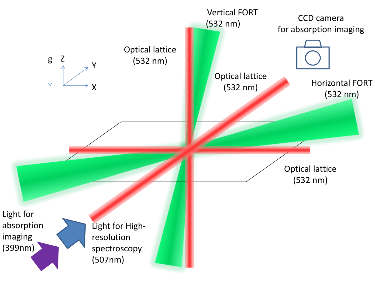
After preparation of the Bose-Einstein condensate (BEC), we adiabatically ramped up a 3D cubic optical lattice generated by three orthogonal, retro-reflected laser beams also having 532-nm wavelength and propagating along the X-, Y-, and Z-axes. The number of atoms before loading onto the optical lattice was stabilized from to .
The experimental procedures for the high-resolution spectroscopy and TOF measurements, including atom loading onto the optical lattice, are shown in Figs. 2 and 3, respectively.
In the first 100 ms of loading, the optical lattice depth was increased to 5 , where the recoil energy , with being the Planck constant and the optical lattice wavelength (532 nm). Then, we increased the final lattice depth of in ms, with the FORT powers being kept constant.
II.2 Preparation of various atomic entropies
One of the important considerations in our experiment was preparation of cold atoms with various atomic entropies in the same experiment setup. We controlled the atomic entropy by changing the FORT depth in the final stage of evaporative cooling. Because the FORT depth depends on the horizontal FORT power, we in fact controlled the final horizontal FORT power in this manner. However, the trap frequencies also depend on the FORT power; therefore, we changed the horizontal FORT power during adiabatic loading onto the optical lattice in the first 100 ms (see Figs. 2 and 3).
Because direct measurement of the atomic entropy in the optical lattice is difficult, we estimated this property from the initial atomic entropy and heating during lattice loading. The initial entropy in a FORT harmonic trap is [13]
| (2) |
where is the atom number; is the atomic temperature in the FORT, which can be directly measured via a TOF method; is the critical temperature; is the zeta function; and is the Boltzmann constant. Here,
| (3) |
where is the geometric mean of the three trap frequencies and is the Planck constant divided by .
To estimate the additional atomic heating during loading onto the optical lattice, we measured the entropy and atom number after adiabatically ramping down the optical lattice in reverse order (see Appendix B). We assumed that the entropy per atom in the optical lattice, , was written as in Eq. (4), using the entropy before (after) loading onto the optical lattice ():
| (4) |
We obtained the atomic entropy by taking five TOF images and calculating each atomic entropy; these values were then averaged.
III Method for Measuring Kinetic-Term Ensemble Average: Fourier Transformation of TOF Signal
Here, we present a method for obtaining the ensemble average of the first term in Eq. (1) (the kinetic term) . We found that can be simply measured from TOF images. The atomic-density distribution after the TOF is given by [14, 15]
| (5) |
where is the atom mass, is the Fourier transformation of the Wannier function in the lowest Bloch band , and = . The structure factor is expressed as
| (6) |
where indicates the site position with index in the optical lattice and represents the ensemble average. The second term in the exponential, , introduces the effect of the finite TOF. This term corresponds to the quadratic term in the Fresnel approximation of near-field optics [16].
Details of our derivation are given in Appendix C. Here, for simplicity, we first consider the one-dimensional case and ignore the finite TOF effect. Equation (6) is then expressed as
| (7) |
Note that we omit the “TOF” label for simplicity in this section. We assume that = and
| (8) |
Next, we define the kinetic energy , where and are the annihilation and creation operators of the Bloch states and . The quasi-momentum runs over the first Brillouin zone only and satisfies the periodic boundary condition Here, is the number of lattice sites along the X-axis and is the lattice spacing (266 nm). We straightforwardly obtain through a Fourier transformation of in the first Brillouin zone, such that
| (9) | |||||
where . Equation (9) implies that the energy of the lowest Bloch band is . To our best knowledge, the above Eq. (9) has not been explicitly reported to date, despite its importance and simplicity. In the present work, this simple relation allows us to successfully evaluate the kinetic energy from experimental observation.
In the experiment, we obtained a two-dimensional (2D) atomic-density distribution , because the TOF signal was integrated in the probe direction (which we took to be the Y-axis). From the atomic linear densities along the X- and Z-axes, we obtained and by fitting of the function, where the Wannier function was obtained by numerically calculating the lowest band of the optical lattice for non-interacting atoms. We consider the structure factor of the form , which is depicted in Fig. 4 ( are fitting parameters).

Then, we obtained the ensemble averages of the kinetic energy () from (), and assumed that the total-ensemble average of the kinetic term was
| (10) |
Note that it is possible to obtain non-local atomic correlations ( = ) using the method shown here. As a demonstration, we directly determine the coherence length in Appendix D. In addition, the 2D atomic correlation can be obtained using the 2D Fourier transformation.
III.1 Effect of finite TOF
The effect of a finite TOF arises from the term in Eq. (6). Instead of adding this effect to TOF image in order to directly compare the experimental results [17], we experimentally evaluated the total site number along the axis () in order to remove this effect. Details are given in Appendix C. The basic concept is that it is possible to evaluate the true value (i.e., the infinite TOF) from experimental measurements with several TOFs through extrapolation. In this work, we measured the atom correlation of , where was 1, 2, 3, 4 and was set to TOFs of 14 and 18 ms. Then, ( = 1, 2, 3, 4) and the total site number along the axis were obtained through fitting using equations similar to Eq. (42). For a TOF of 14 (18) ms, a reduction of 6 (4) % in the value of from its value for an infinite TOF was estimated. Note that this finite TOF effect was experimentally checked using datasets for various TOFs, with the other experimental parameters unchanged, and the validity of our result was confirmed (see Appendix C). Because the correction of the finite-TOF effect is model-dependent, so we consider estimated deference between the values before and after the correction as a systematic error.
It is noted that the finite-TOF effect scales as for whole sites. However, it scales as for neighbor sites, which contribute to the kinetic energy, and resulted in highly-suppressed finite-TOF effect for measurement of atom correlation in the neighbor sites. The corrections itself are estimated to be within 6% and therefore the selection of the assumption of the density function is not so critical.
III.2 Effect of inter-atomic interaction during TOF
The discussion above is based on the Wannier states of non-interacting atoms. Here we discuss the effect of inter-atomic interaction during TOF. First is the validity of the Wannier function numerically calculated. The kinetic energy of non-interacting atoms in the lowest band of the optical lattice is estimated to be , where is the oscillation frequency at the bottom of the lattice potential [15]. The ratio of the interaction energy to the kinetic energy , i.e.,
| (11) |
determines the relative importance of the inter-atomic interaction during the TOF. The ratio was mostly far lower than 1 under our experimental conditions. Our calculations indicate that takes the maximum value of 0.25 at 7 depth in the case of triple occupancy, , for which the population fraction is less than 0.1 (see Sec. VI). Therefore, the effect of the inter-atomic interaction was negligible in our experiment.
IV Method to Measure Ensemble Average of Interaction Term: Atom-Number-Projection Spectroscopy
We have developed a new method of atom-number-projection spectroscopy, which enables direct measurement of the number of multiply occupied sites at any optical lattice depth and, hence, accurate evaluation of the interaction term across the weakly to strongly interacting regimes. One may wonder whether such a new method is truly necessary, because information on the numbers of n-occupied sites is straightforwardly obtained through high-resolution spectroscopy for the atoms in a deep optical lattice. In fact, site-occupancy-resolved spectra in a deep optical lattice have already been reported in [10] for the – transition, in [19, 20] for the –3P0 transition of Yb, and in [21] for the –3P0 transition of strontium (Sr). In contrast, as shown in Fig. 5 (a), a single, broad spectrum of coexisting SF and normal components was observed in the case of a shallow optical lattice depth [10]. The hopping time at small optical lattice depth (0.6 ms for 5 depth) is comparable to the excitation time (0.5 ms in the case of Fig. 5); therefore, the peaks of the observed spectra are not well separated.
A shorter excitation time is preferable for suppressing atom hopping during excitation. However, this causes spectral broadening of the resonance lines, significantly exceeding the separation between peaks under our conditions. The frequency separation of the peaks is given by the collisional shift: . Here, is the on-site two-body interaction and is the two-body interaction between the state () and state ().
As an alternative, we have developed a new method: atom-number-projection spectroscopy. In this approach, we increase the optical lattice depth quickly in order to freeze atom hopping, and then irradiate the atoms with an excitation light pulse. The ramp-up time is ms from 5 to 15 and is faster than atom hopping, but sufficiently slow to prevent atom excitation into the higher band of the optical lattice ( 20 kHz). Figure 5(b) shows spectra obtained using the atom-number-projection method, and the site-occupancy-resolved spectrum was indeed acquired for the shallow optical lattice. Here, -occupancies of up to five were distinguished with a separation of approximately . The lower the resonance frequencies, the higher the occupation numbers n became. Note that our excellent resolution that allows different site occupancies to be distinguished is obtained by exploiting the optical transition between the and () electronic states of Yb atoms, which have quite different two-body interactions of = -8.5 kHz and = 3.2 kHz at 15. An additional advantage is that neither the nor () state is sensitive to a magnetic field, which enables acquisition of narrow spectra free from possible broadening due to magnetic field inhomogeneity.
Typical spectra are shown in Fig. 6, with the corresponding TOF images.

Naively, the area of each resonance in the spectrum is thought to be linearly proportional to the atom population in the corresponding occupancy of the optical lattice. The excited state population of the -occupied site after the excitation time is [22]
| (12) |
where are the (angular) Rabi frequencies and are the decay rates, with both parameters being dependent on . Note that resonance frequency shift yields excitation of one atom only, even for an n-occupied site. Thus, we must divide the by when we consider the excited state population per atom. If the spectral width of each resonance is the same, the area for the -occupied site is linearly proportional to
| (13) |
where is the total atom number at the -occupied site.
In the case of non-interacting atoms, the Rabi frequencies should be proportional to because of the super-radiance or bosonic stimulation effect [23, 24]:
| (14) |
In addition, when the excitation time is much shorter; i.e., and , we obtain
| (15) |
Because and were fixed in our experiment, the relative strengths of the areas indicate the relative atom number distributions among the sites in the optical lattice.
We experimentally examined the occupancy-dependent properties of the finite lifetime and transition probability in order to evaluate the total atom number at the -occupied sites accurately. We discuss these properties in the following subsections. The details of the experimental parameters and procedures of our atom-number-projection spectroscopy are described in Appendix E.
IV.1 Occupancy-dependent lifetime measurement
The radiative lifetime of the state is approximately 15 s, which introduces negligible atom loss during our atom-number-projection spectroscopy. Instead, the dominant loss process is the inelastic collision between the atoms in the and states, which is induced by the fine-structure, principal-quantum-number, and Zeeman-state changing collisions [25]. Note that the magnetic sublevel () we use is not the lowest Zeeman-energy level. Further, our excitation time of 0.3 ms is not negligible compared to the occupancy-dependent decay times, as shown in Fig. 7; therefore, we actually measured the decay time to determine the correction factors for our atom-number-projection spectroscopy.
First, approximately BEC atoms were loaded into the shallow optical lattice (5). Then, the lattice depth was suddenly increased to 15 in 0.1 ms. Next, we excited the atoms at the -occupied sites and measured the number of atoms remaining in the state after a given hold time. The results are shown in Fig. 7.
We fit the data with single-exponential decay curves. The measured decay constants of the -occupied states () were , , and ms, respectively. For the site, we could not find any decay within our short hold time. Therefore, it was necessary to correct the occupied atom number for the cases of , and sites only, for which the correction factors were , , and , respectively.
IV.2 Occupancy-dependent Rabi oscillation frequency
For the non-interacting cases, the Rabi frequencies should be proportional to . In the presence of the inter-atomic interaction, the situation is less simple and the -dependence of the Rabi frequency is modified in general by broadening of the Wannier function due to inter-atom interactions [9, 19]. Such a modification was indeed observed in our system [10]. Here, we carefully evaluated the -dependent Rabi frequency experimentally.
To observe clear Rabi oscillations, we excited the atoms with a relatively strong laser power of 4 mW, which corresponds to approximately 100 ; the expected Rabi frequency at was approximately kHz. The observed Rabi oscillations are shown in Fig. 8.
The fitting lines were drawn by solving the optical Bloch equations numerically, assuming that the detuning was zero:
| (16) | |||
| (17) | |||
| (18) |
where , , , and is the density matrix of the -occupied sites. The Rabi frequencies of the -occupied sites were (), (), (), and kHz (). The measured relative strength among the occupancy-dependent Rabi frequencies was used as a correction factor to estimate the atom-number distribution in our atom-number-projection spectroscopy.
V Possibility of Measuring Ensemble Average of Potential Energy Term
The third term of Eq. (1), the potential energy term, is from the inhomogeneous trap potential due to the FORT beams and optical lattice lasers. Although the spatial distribution of the atoms in a trap for a single 2D plane can be directly measured using a high-spatial-resolution in situ imaging technique such as a quantum gas microscopy [11, 26], our imaging resolution was insufficient to accurately extract the spatial distributions of the atoms in our 3D optical lattice.
VI Experimental Determination of Bose-Hubbard Energies
Here, we present our main experimental results. Figure 9 shows the comprehensive measurements of the kinetic energy divided by the hopping matrix element per atom, i.e., the ensemble average of the term per atom for lattice depths from 5 to 18 across the weakly to strongly interacting regimes as a function of the atomic entropy per atom. When the lattice depth was 10.6, was equal to , which is the critical lattice depth for the SF-MI transition at .
Note that the per atom must range between 6 and –6 for the 3D optical lattice. The maximum and minimum values of 6 and –6 correspond to the atom condensation at and , respectively. Here, denotes the quasi-momentum.
Naturally, the expected behaviors were successfully observed in our experiment data, as shown in Fig. 9. In a shallow optical lattice at sufficiently low entropy, almost all atoms should be condensed at , corresponding to a close to 6; this is clearly apparent for the lower entropy data shown in Figs. 9(a)–(c). With increased optical lattice depth, decreases and approaches zero because of the repulsive inter-atomic interaction (); this is also clearly apparent as a general tendency of the data in Fig. 9. In a deep optical lattice, all atoms are isolated and there is no phase coherence in a MI state. The atoms are distributed over the entire first Brillouin zone, corresponding to ; this behavior can be recognized in the data shown in Fig. 9(j) and (k). When the atomic entropy increases, should decrease because of the thermal excitation to energetically higher states with larger at any lattice depth. Again, this behavior can be clearly recognized as the general tendency of the data in Fig. 9.
Figure 10 shows the comprehensive measurements of the interaction energy divided by per atom; namely, the ensemble average of the term per atom, again for lattice depths from 5 to 18 across the weakly to strongly interacting regimes as a function of the atomic entropy per atom.
Again, the naturally expected behaviors of were successfully observed in our experiment data (Fig. 10). In a shallow optical lattice, the atom hopping process is dominant and the atoms are delocalized at multiply occupied sites, although the average filling-factor value is approximately unity. This case yields a larger value of , and this is clearly apparent in Figs. 10(a)–(c), for example. When the optical lattice depth is increased, the repulsive inter-atomic interaction plays a more important role in suppressing the atom hopping, yielding a decrease in . This is clearly apparent as a general tendency of the data in Fig. 10. In a deep optical lattice, the atoms are isolated in an MI state with unit filling, which corresponds to , as apparent in the data in Figs. 10(h)–(k). In the SF state, should decrease when the atomic entropy increases, because the thermal excitation yields expansion of the atomic cloud and a decrease in the multiply occupied sites. This can be clearly recognized again as the general tendency of the data in Fig. 10.
The population fractions, which could be directly measured by our atom-number-projection spectroscopy technique, elucidated further details of the atom number distribution in an optical lattice site. The population fractions at various lattice depths as functions of the atomic entropy are shown in Fig. 11.
We found occupancy, although small, at small lattice depths only, as shown in Figs. 11(a)–(c). In Figs. 11(a)–(g), decreases in the and populations accompanied by an increase in the population can be clearly observed in accordance with the atomic entropy and lattice depth increase; this can be interpreted as originating from disappearance of the SF components.
VII Numerical Calculation Benchmark
The obtained experimental results can be used as benchmarks for state-of-the-art numerical methods of quantum many-body theory. As an illustrative example, in this section, we compare the measured kinetic and interaction energies as well as the population fractions of n-occupied sites with numerical calculations based on the Gutzwiller and cluster-Gutzwiller approximations.
VII.1 Gutzwiller approximation
In this subsection, we explain two numerical methods based on Gutzwiller approximation. One is a simple finite-temperature Gutzwiller approximation, where the effects of boson hopping are approximated as a mean field [10, 27]. This is a simple local approximation obtained by solving the localized Hamiltonian with the exact diagonalization method at finite temperature. Local thermodynamic quantities such as double occupancies can be well approximated by this calculation [10, 27]. Another method is a cluster-type extension of this local approximation; that is, some of the hopping terms are included in the exact diagonalization calculation. This cluster Gutzwiller approximation allows us to consider the kinetic energy much more effectively than the local approximation.
In a local Gutzwiller approximation, the Bose–Hubbard Hamiltonian is approximated by the set of effective local Hamiltonians
| (19) |
under a self-consistent condition at thermal equilibrium for each local Hamiltonian. The mean field is given by
| (20) |
where , , and for adjacent and sites, and otherwise. The Hubbard parameters, including , , and , are determined ab initio from Wannier functions. We use the exact diagonalization method to solve these local Hamiltonians at finite temperature, where is the number of lattice sites. Here, we solve the finite Hilbert space by truncating states with a large number of bosons () at each lattice site. The truncated states are negligible, because the on-site interaction suppresses them, even for shallow lattices.
Under the self-consistent conditions, we calculate the double occupancy , potential energy , and kinetic energy . A non-local quantity such as is now approximated as a product of the local quantities . The kinetic energy under the local approximation corresponds to the energy of the condensed bosons
| (21) |
and the energies of the uncondensed normal states (normal fluid and MI) that appear as a result of the thermal fluctuation and correlation effects
| (22) |
are completely neglected. Thus, the local Gutzwiller approximation inevitably underestimates the kinetic energies at middle-depth lattices. In contrast, local quantities can be directly calculated using the exact-diagonalization method, which allows us to properly consider the effects of the normal states.
In a cluster-Gutzwiller approximation, the local Hamiltonians are extended to the two-site cluster Hamiltonians including a hopping term:
| (23) |
We use exact diagonalization to solve the cluster Hamiltonian by truncating states with more than eight bosons in each cluster. We also extend two self-consistency conditions in the cluster Hamiltonian :
| (24) | |||||
| (25) |
That is, to avoid double counting of the effects of , we subtract this term from the mean fields and . We solve cluster Hamiltonians for the 3D cubic lattice, and local quantities such as are obtained from the average of six clusters for sites adjacent to . Note that, when the self-consistency conditions are satisfied, the local quantities for the th site in the agree well with each other. For , we can calculate a non-local quantity , allowing us to obtain a kinetic energy that includes the effects of normal states, .
VII.2 Comparison of experiment and theory
We compared the measured kinetic and interaction energies as well as the population fractions of n-occupied sites with numerical calculations of the Gutzwiller and cluster-Gutzwiller approximations in finite entropy (finite temperature). Note that the trap potentials and particle numbers in the calculations were the same as those of the experiments and there were no fitting parameters in the calculation.
The dashed blue and dotted green lines in Fig. 9 represent the numerical results for the term obtained using the Gutzwiller and cluster-Gutzwiller methods, respectively, with different atom numbers ( to ) being represented by the shaded areas. Although we can observe overall agreement between the experimental data and numerical calculations for the overall lattice depth and atomic entropy, our measurement was highly consistent with the numerical calculation using the cluster-Gutzwiller method.
We discuss here possible origins of slight deference between the measured and numerical values appeared at the shallow optical lattice. One of the possibility is imaging resolution of TOF images. We consider the condensate atoms with zero momentum for simple explanation, which has a by definition. The finite imaging resolution broadens the measured momentum distribution around the zero momentum. We consider a Gaussian point-spread function of as the structure factor , where and is a resolution and assume . By simple calculation, the measured should be . If 5 , 5.7 and therefore the finite resolution is not negligible when lattice depth is shallow and the system has large . Similar broadening might also occur when the interaction energy is transfered to the kinetic energy, which is discussed in Ref. [18], where hydrodynamic expansion occurs around low-momentum part and results in peak broadening.
Both Gutzwiller methods exhibited similar results at shallow lattice depths, but differences emerged at deeper lattice depths and in the large-atomic-entropy regime. The technical difference between the Gutzwiller and cluster-Gutzwiller methods lies in the handling of the atomic correlation of the nearest-neighbor sites. In the case of the Gutzwiller method, the atomic correlation between the nearest-neighbor sites is from the SF component; thus, the atomic correlation of the thermal component is not considered. Therefore, testing with our experimental data revealed that the atomic correlation between the nearest-neighbor sites from thermal fluctuation is indeed important in higher-entropy and deeper-lattice cases.
The dashed blue and dotted green lines in Fig. 10 represent the numerical results for the term obtained using the Gutzwiller and cluster-Gutzwiller methods, respectively, with different atom numbers ( to ) being represented by the shaded areas. In contrast to the term, the numerical results obtained using both the Gutzwiller and cluster-Gutzwiller methods were similar. Again, overall agreement between the experimental data and numerical calculations was obtained for almost all lattice depths and atomic entropy. However, differences between the measured and numerical values appeared when the optical lattice was deeper, as shown in Figs. 10(g)–(k). Although we are uncertain of the origin of these differences, we suspect that double occupancy may have occurred in the deeper optical lattice regime, because of the slight breaking of the adiabatic condition during lattice loading [28, 29, 30]. Our ramp-up time of approximately 200 ms should be sufficient to reach local thermalization, but may be too short for global-mass redistribution in the deep-lattice case. Note that the non-negligible atomic heating and loss observed for longer loading times limits us to this ramp-up time.
Numerical calculation of the population fractions as functions of the atomic entropy per atom was also performed, at various lattice depths. The solid red, dashed blue, dotted green, and dashed-dotted yellow solid lines in Fig. 11 show the numerical results for the normalized areas of , , , and occupied sites, respectively. Here, the total of the normalized areas is equal to unity. We found excellent agreement between the experiment and numerical calculations, especially up to the critical lattice depth of 11 (Figs. 11(a)–(f)), but a certain disagreement at deeper lattice depth (Figs. 11(g)–(k)), which can be attributed to the same reason discussed with regard to the disagreement for above.
We also investigated the total internal energy per atom (i.e., the sum of the kinetic and interaction energies) at various lattice depths as a function of atomic entropy (Fig. 12).
The numerical results obtained using both Gutzwiller and cluster-Gutzwiller methods were similar. The difference between the two numerical calculations of was not small at deeper lattice depth; however, the calculated kinetic energies of were almost identical because of the small values of at deeper lattice depth. The measured values were consistent with the numerical results.
VIII Conclusions and Future Prospects
We have presented, to our best knowledge, the first measurements of the ensemble averages of both the kinetic and interaction energies of the 3D Bose–Hubbard model at finite temperature and various optical lattice depths by establishing a protocol to accurately extract the ensemble average of the kinetic energy from a TOF signal and by developing a new method of atom-number-projection spectroscopy to accurately evaluate the interaction term across the weakly to strongly interacting regimes. Our measurements showed rather strong dependence on the atomic entropy, except in the strongly correlated region. This implies that information on the equilibrium state of the Bose–Hubbard system can be obtained from these measurements. In addition, our atom-number-projection spectroscopy method offers information on the relative populations of the multiply occupied sites from the population fractions. In this study, using these population fractions, we observed a decrease in the and populations when the atomic entropy and lattice depth increased; this behavior should be due to the disappearance of the SF components. The obtained experimental results for the internal energies as well as the population fractions were compared with numerical calculations based on finite-temperature Gutzwiller and cluster-Gutzwiller methods; hence, we obtained agreement between the experiment and cluster-Gutzwiller calculation without fitting parameters. This indicates the important role of the atomic correlation between the nearest-neighbor sites through thermal fluctuation, especially in higher-entropy and deeper-lattice cases.
Measurement of the internal energy for various entropies offers a novel possibility of estimating the atomic temperature in a lattice, which is the most important parameter governing the thermal equilibrium state. If the total internal energies, i.e., the kinetic, interaction, and potential terms, are measured experimentally, one can determine the temperature using the thermodynamic relation , where is the total internal energy and is the atomic entropy. We have checked this proposal numerically (see Appendix F). This possibility is important, because the temperature in an optical lattice has only been estimated indirectly to date, through comparison of the experimental results and theoretical calculation. Finally, the methods demonstrated here are not particular to Bose gases in equilibrium, but can be applied to Fermi gases, Bose–Fermi mixtures, and even non-equilibrium states.
This paper is, to the best of our knowledge, the first report of experimental determination of both the kinetic and interaction energies of quantum many-body systems. This study offers a unique advantage of cold atom system for “quantum simulators”.
Acknowledgements.
We thank H. Shiotsu, K. Takiguchi, and J. Sakamoto for experimental assistance. This work is supported by MEXT/JSPS KAKENHI, Grant Numbers JP25220711, JP26247064, JP16H00990, JP16H01053, JP16H00801, JP18H05228, JP18H05405; and the Impulsing Paradigm Change through Disruptive Technologies (ImPACT) program; and CREST, JST JPMJCR 1673; and the Matsuo Foundation. Y. Takasu and Y.N. equally contributed to this work.Appendix A Energy diagram and scattering length of Yb
Figure 13 shows the Yb schematic energy diagram (not scaled) relevant to the experiment.
Throughout this paper, we used the value of the scattering length of of 5.55 nm [31].
Appendix B Additional information of our Experimental Setup and Procedure
The beam waists ( radii) of the horizontal FORT were approximately 15 and 33 m and the short axes of the ellipses were oriented along the Z-axis. The beam waists of the vertical FORT were approximately 43 and 126 m, and the short axes of the ellipses were oriented along the X’-axis, where the X’-axis formed an angle of 45 degrees relative to both the X- and Y-axes. The beam waists of the lattice beams were approximately 100 m. The FORT trap frequencies were (27.9, 130, 162.5) Hz after the lattice loading.
The measurement procedure for the entropy and atom number after adiabatically ramping down the optical lattice in reverse order is shown in Fig. 14.
Appendix C Kinetic term
In this section, we label the atom momentum as for simplicity. The atomic density distribution after the TOF , i.e., , is
| (26) |
The atomic momentum after the TOF is calculated from the positions of the atoms and = . Here, is the Fourier transformation of the Wannier function in the lowest Bloch band and
| (27) |
The structure factor is
| (28) |
First, we consider the integral of along the Y-axis in position space:
| (29) |
where , , and . Then,
| (30) |
where we use the orthogonality of the Wannier functions,
| (31) |
with = 0, , , , and being the lattice spacing.
By applying Eq. (30) to Eq. (29), we obtain
| (32) |
where is the Kronecker delta. That is, =1 if and only if ; otherwise, .
Similarly, we obtain the linear atomic density is
| (33) |
and
| (34) |
where is the total number of atoms.
C.1 Case I: Infinite TOF
First, for simplicity, we consider the case in which the TOF is infinite and the Fresnel term is negligible. In this case, the linear atomic density is (see also Eq. (33)) as follows:
| (35) |
Therefore, the ensemble average of the atomic correlations of nearest-neighbor sites, , is obtained using Fourier transformation in the first Brillouin zone, where
| (36) |
Similarly,
| (37) |
Noted that if TOF images are symmetric with respect to the , and therefore is real. This is valid if the hopping matrix element is real and the system is in equilibrium states (strictly speaking, if the system has time-reversal symmetry), because the kinetic energy itself is required to be real. This assumption is invalid for some special cases, for example, non-equilibrium states with non-zero total quasi-momentum, and equilibrium states with an artificial gauge field (complex hopping matrix elements) [33]. In these cases, however, must be complex and we believe that the kinetic energy can be obtained using the above procedure, if the Wannier functions are well defined.
Similarly,
| (38) |
C.2 Case II: Finite TOF
Under our experimental conditions, the Fresnel term is non-negligible because there is a finite TOF. However, the effect is small; therefore, we can consider it to be a correction factor:
| (39) |
Now, we assume that is independent of site index and have a average value , and the summation is from to and ,
| (40) |
where . We here defined the correction factor as
| (41) |
where we assume that is real and therefore the correction factor is also real. Similarly, we obtain the relation on the long-range atomic correlation with the lattice separation ,
| (42) |
The total site number and are obtained by fitting the long-range atomic correlation by use of the experimental data with various lattice separation and several TOFs. In our experiment to measure the ensemble average of the kinetic term, the TOFs were 14 and 18 ms. Figure 15 shows our typical measured long-range atomic correlation and the fitting curves obtained using Eq. (42).
Finally, by fitting with Eq. (45), we obtain the coherence length .
The correction factor is shown in Fig. 16 as the solid red line using our experimental parameters.
The deviation by the Fresnel effect is estimated to be about 6% (4%) for 14 ms (18 ms) TOF. It is to be noted that the correction factor also depends on total atom size and monotonically decrease with the limit .
Here we assume that the atom correlation have the average value of and unique atom density, which is valid for a Mott insulating case. However, this is not a unique possible assumption and the calculated correction factor depends on models. For reference, we calculated a correction factor based on the assumption of and is shown in Fig. 16 as the blue dotted line, where we assumed that density distribution the Gaussian function and the is a correlation length [36]. In this model, because of large atom density around the center of the trap, effective size of atoms are small compared to the model with unique atom density, and therefore small correction factor obtained. Apart from non-realistic cases (namely, atom density around the edge of the trap is large compared to the one in the center), atoms with unique density have the largest effective size, and it results in the largest correction factor. These estimations show that the maximum of the correction factor may obtain from the model with unique atom density. Therefore we also use estimated difference between the values before and after the correction as systematic errors in order to cover the uncertainty of atoms density distribution in the trap. In a coexistence case of SF-Mott phase, the correction are expected within the systematic errors.
Appendix D Measurement of visibility, width, and coherence length
The widely used experimental observables from the TOF images are the visibility (Fig. 17) and peak width (Fig. 18). Figures 17(a–k) show the visibilities as functions of atomic entropy.

The visibility is defined as [34, 35]
| (43) |
where is the maximum density at the first interference peak. The minimum density is measured at the same distance, but in a diagonal direction from the central peak (see also, Fig. 17(l)). It is clearly apparent that the visibility is large at small lattice depth and decreases as the lattice depth increases. The dependence of the visibility on the atomic entropy is small.
Figure 18 shows the widths of the central peaks as functions of the atomic entropy.
The central peak width is one of the most commonly used parameters to evaluate the phase coherence. If the TOF is sufficiently long to neglect the Fresnel effect (see Eq. (7)), the structure factor is
| (44) | |||||
where is the wavefunction of the SF component. It is naturally expected that a larger phase coherence corresponds to a sharper peak width. One can clearly see that the central peak is sharp at shallow lattice depth and increases with lattice depth. The dependence of the peak width on the atomic entropy is small.
While these measurements have been standard methods in the study of the SF-MI transition, the new internal energy measurements of the Bose-Hubbard system demonstrated in this work provide a useful method of investigating the SF-MI transition, as shown in the main text.
Figure 19 shows the coherence lengths as functions of the atomic entropy.
Our Fourier transformation method enables us to consider the long-range atomic correlation of more than just the nearest-neighbor sites. Here, is defined as [36]
| (45) |
where is the atomic density at site . The value of is obtained by fitting Eq. (45) to our measured ensemble average of the long-range atomic correlation (see Appendix C). Note that is large at a small lattice depth and decreases with increased lattice depth. As expected, is near one lattice spacing around the quantum critical point ( for ). This behavior also shows the quantum phase transition between SF and MI.
Appendix E Atom-number-projection spectroscopy procedure
We used the transition from the () state to the () () state for high-resolution spectroscopy. Neither the nor the () state is sensitive to magnetic fields, because lacks a nuclear spin; this enabled us to obtain narrow spectra in the absence of inhomogeneous broadening resulting from an external magnetic field.
Light for the excitation was generated through frequency doubling of an external-cavity laser diode at 1014 nm, locked to an ultralow expansion cavity, which had slow-frequency drift with a typical rate of approximately 1 kHz/h. The linewidth of the excitation laser was less than 1 kHz.
After atom projection to a large optical depth of , as described above, we applied an excitation pulse. The pulse width was 0.3 ms. The incident power was approximately 100 W and the beam waist was approximately 50 m. The intensity was W/ and the Rabi frequency was approximately 0.3 kHz. To excite the - () transition, the excitation light propagating along the Y-axis was polarized along the Z-axis and we applied a magnetic field of mG in the -X+Y direction.
After applying the excitation light, we removed the remaining atoms in the state with a light that resonated with the -() transition for 0.3 ms. Then, atoms in the state were transferred to the state with two repumping lights resonant with the - () and ()-() transitions. Finally, the number of atoms in the state was measured using a fluorescence imaging technique employing a magneto-optical trap with the - transition.
Typical spectra have already been shown in Figs 5 (b) and 6. Our spectra were obtained after projection into the lattice depth of ; thus, the positions of each peak relative to the peak were fixed. Therefore, our spectra covered four peaks corresponding to .
The spectral areas were obtained by fitting using a sinc function, because our excitation light pulse was rectangular and the resulting broadening from Fourier transformation of the rectangular function was dominant. The correction factors from the reduced Rabi frequencies and finite lifetimes of atoms in the state ( = ) were considered. We took three or more spectra and calculated the atomic distribution for each one; then, these data were averaged. To save time on our experiment, only several data points in the vicinities of peaks were taken. A period of approximately 20 min was required to obtain one spectrum and the long-term drift was negligible for the time scale.
Appendix F Possible Temperature Estimation from Energy Measurements
Although the atomic temperature in an optical trap without an optical lattice can be easily measured using a TOF method, the atomic temperature in an optical lattice is estimated only indirectly through comparison of the experimental results and theoretical calculation. In the higher-temperature region, estimation of the atom temperature from the in situ atom distribution [37] and spin-gradient thermometry [38] has been demonstrated, as well as use of quantum gas microscopy [37].
Alternatively, however, if the total internal energies are measured experimentally, one can determine the temperature using the thermodynamic relation
| (46) |
where is the total internal energy and is the atomic entropy.

In our experiment, evaluation of the potential energy is difficult, as mentioned.
Figure 20 (a) shows the temperature estimated using the relation . The ensemble averages of the kinetic, interaction, and potential terms for estimation were obtained from the Gutzwiller approximation. This result is consistent with the temperature directly obtained using numerical calculation with the Gutzwiller approximation and shown in Fig. 20 (b).
The contribution of the potential term comes from the trap potentials and the Gaussian envelope of the optical lattice lasers. This is because both external potentials are quadratic terms with respect to the lattice index; that is, , where is the overall (mean) trap frequency as a function of lattice depth and is the central position of the overall external potential.
Therefore, the Bose-Hubbard-model Hamiltonian is expressed as
| (47) |
where is the total atom number and . Note that , , and are known functions that depend only on .
We apply the Hellmann–Feynman theorem [39, 40] to the ensemble average of the Hamiltonian :
| (48) |
where is the atomic entropy in the optical lattice and
| (49) |
The values of , , and are experimentally observed and given by
| (50) | ||||
| (51) | ||||
| (52) |
and we omit for simplicity in this section (that is, instead of ). Therefore,
| (53) |
where is the atomic temperature.
Even if the ensemble average of the potential terms is unavailable, the atomic temperature can be estimated. To demonstrate this, we consider the normalized operator and its ensemble average.
| (54) |
In contrast,
| (55) |
Because
| (56) |
the dependence of on is
| (57) |
Using Eq. (54),
| (58) |
Equation (58) shows that we must obtain the dependencies of and on the atom entropy because , , and are all known functions. Therefore, direct measurement of the potential term is not necessary to estimate the atomic-temperature dependence. When we know the absolute atomic temperature at a certain lattice depth , we can estimate the other absolute atomic temperatures through integration of Eq. (58).
References
- [1] M. P. A. Fisher, P. B. Weichman, G. Grinstein, and D. S. Fisher, Phys. Rev. B 40, 546 (1989).
- [2] D. Jaksch, C. Bruder, J. I. Cirac, C. W. Gardiner, and P. Zoller, Phys. Rev. Lett. 81, 3108 (1998).
- [3] I. Bloch, J. Dalibard, and W. Zwerger, Rev. Mod. Phys. 80, 885 (2008).
- [4] I. Bloch, J. Dalibard, and S. Nascimbène, Nature Physics 8, 267 (2012).
- [5] M. Greiner, O. Mandel, T. Esslinger, T. W. Hänsch, and I. Bloch, Nature 415, 39 (2002).
- [6] B. Capogrosso-Sansone, N. V. Prokof’ev, and B. V. Svistunov, Phys. Rev. B 75, 134302 (2007).
- [7] S. Fölling, F. Gerbier, A. Widera, O. Mandel, T. Gericke, and I. Bloch, Nature 434, 481 (2005).
- [8] W. S. Bakr, A. Peng, M. E. Tai, R. Ma, J. Simon, J. I. Gillen, S. Fölling, L. Pollet, and M. Greiner, Science 329, 547 (2010).
- [9] G. K. Campbell, J. Mun, M. Boyd, P. Medley, A. E. Leanhardt, L. G. Marcassa, D. E. Pritchard, and W. Ketterle, Science 313, 649 (2006).
- [10] S. Kato, K. Inaba, S. Sugawa, K. Shibata, R. Yamamoto, M. Yamashita, and Y. Takahashi, Nature Comm. 7, 11341 (2016).
- [11] W. S. Bakr, J. I. Gillen, A. Peng, S. Fölling, and M. Greiner, Nature 462, 74 (2009).
- [12] K. V. Krutitsky, Physics Reports 607, 1 (2016).
- [13] C. J. Pethick and H. Smith, Bose-Einstein Condensation in Dilute Gases, 2nd ed. (Cambridge University Press, 2008).
- [14] P. Pedri, L. Pitaevskii, S. Stringari, C. Fort, S. Burger, F. S. Cataliotti, P. Maddaloni, F. Minardi, and M. Inguscio, Phys. Rev. Lett. 87, 220401 (2001).
- [15] F. Gerbier, S. Trotzky, S. Fölling, U. Schnorrberger, J. D. Thompson, A. Widera, I. Bloch, L. Pollet, M. Troyer, B. Capogrosso-Sansone, N. V. Prokof’ev, and B. V. Svistunov, Phys. Rev. Lett. 101, 155303 (2008).
- [16] E. Toth, A. M. Rey, and P. B. Blakie, Phys. Rev. A 78, 013627 (2008).
- [17] L. Vidmar, J. P. Ronzheimer, M. Schreiber, S. Braun, S. S. Hodgman, S. Langer, F. Heidrich-Meisner, I. Bloch, and U. Schneider, Phys. Rev. Lett. 115, 175301 (2015).
- [18] V. A. Kashurnikov, N. V. Prokof’ev, and B. V. Svistunov, Phys. Rev. A 66, 031601 (2002).
- [19] L. Franchi, L. F. Livi, G. Cappellini, G. Binella, M. Inguscio, J. Catani, and L. Fallani, New Journal of Physics 19, 103037 (2017).
- [20] R. Bouganne, M. B. Aguilera, A. Dareau, E. Soave, J. Beugnon, and F. Gerbier, New Journal of Physics 19, 113006 (2017).
- [21] S. L. Campbell, R. B. Hutson, G. E. Marti, A. Goban, N. Darkwah Oppong, R. L. McNally, L. Sonderhouse, J. M. Robinson, W. Zhang, B. J. Bloom, and J. Ye, Science 358, 90 (2017).
- [22] C. J. Foot, Atomic Physics, Oxford Master Series in Atomic, Optical and Laser Physics (Oxford Univ. Press, Oxford, 2007).
- [23] R. H. Dicke, Phys. Rev. 93, 99 (1954).
- [24] M. Gross and S. Haroche, Physics Reports 93, 301 (1982).
- [25] S. Uetake, R. Murakami, J. M. Doyle, and Y. Takahashi, Phys. Rev. A 86, 032712 (2012).
- [26] J. F. Sherson, C. Weitenberg, M. Endres, M. Cheneau, I. Bloch, and S. Kuhr, Nature 467, 68 (2010).
- [27] S. Sugawa, K. Inaba, S. Taie, R. Yamazaki, M. Yamashita, and Y. Takahashi, Nature Physics 7, 642 (2011).
- [28] J. Zakrzewski and D. Delande, Phys. Rev. A 80, 013602 (2009).
- [29] C.-L. Hung, X. Zhang, N. Gemelke, and C. Chin, Phys. Rev. Lett. 104, 160403 (2010).
- [30] M. Dolfi, A. Kantian, B. Bauer, and M. Troyer, Phys. Rev. A 91, 033407 (2015).
- [31] M. Kitagawa, K. Enomoto, K. Kasa, Y. Takahashi, R. Ciuryło, P. Naidon, and P. S. Julienne, Phys. Rev. A 77, 012719 (2008).
- [32] J. H. Denschlag, J. E. Simsarian, H. Häffner, C. McKenzie, A. Browaeys, D. Cho, K. Helmerson, S. L. Rolston, and W. D. Phillips, Journal of Physics B: Atomic, Molecular and Optical Physics 35, 3095 (2002).
- [33] J. Dalibard, F. Gerbier, G. Juzeliūnas, and P. Öhberg, Rev. Mod. Phys. 83, 1523 (2011).
- [34] F. Gerbier, A. Widera, S. Fölling, O. Mandel, T. Gericke, and I. Bloch, Phys. Rev. Lett. 95, 050404 (2005).
- [35] F. Gerbier, S. Foelling, A. Widera, and I. Bloch, arXiv:0701420 .
- [36] S. Braun, M. Friesdorf, S. S. Hodgman, M. Schreiber, J. P. Ronzheimer, A. Riera, M. del Rey, I. Bloch, J. Eisert, and U. Schneider, Proceedings of the National Academy of Sciences 112, 3641 (2015).
- [37] D. McKay, M. White, and B. DeMarco, Phys. Rev. A 79, 063605 (2009).
- [38] D. M. Weld, P. Medley, H. Miyake, D. Hucul, D. E. Pritchard, and W. Ketterle, Phys. Rev. Lett. 103, 245301 (2009).
- [39] H. Hellmann, Einführung in die quantenchemie (Deuticke, Leipzig und Wien, 1937).
- [40] R. P. Feynman, Phys. Rev. 56, 340 (1939).