SciSports: Learning football kinematics through two-dimensional tracking data

We first consider the case of modeling the movement of one football player in the first match. We assume that this player is not a goalkeeper, since we would like to model movement ranges that span at least half the field. The data provides a player’s $(x,y)$-position at every fixed $100$ milliseconds as long as he remains in the game. Let $\Delta t$ be the time difference between successive timesteps, and let us denote a player’s position in the $(x,y)$ plane at timestep $t$ as $\boldsymbol{x}_{t}$, with the velocity and acceleration as $\boldsymbol{v}_{t}$ and $\boldsymbol{a}_{t}$; they are related by $\boldsymbol{a}_{t}=d\boldsymbol{v}_{t}/dt$ and $\boldsymbol{v}_{t}=d\boldsymbol{x}_{t}/dt$. By approximating these derivatives by finite differences we obtain

We now model the acceleration $\boldsymbol{a}_{t}$. We assume that at each timestep $t$ the acceleration $\boldsymbol{a}_{t}$ is independently and normally distributed with mean $\boldsymbol{0}$ and unknown covariance matrix $\boldsymbol{Q}$ (we write this as $\boldsymbol{a}_{t}\sim\mathrm{N}(\boldsymbol{0},\boldsymbol{Q})$). Since acceleration is proportional to force by Newton’s second law of motion, this induces a normal distribution on the corresponding force exerted by the player, and the exponential decay of its tails translate to natural limits imposed on muscular work output.

In view of (3.1), we take position and velocity $(\boldsymbol{x}_{t},\boldsymbol{v}_{t})$ as our underlying state vector, and we consider the following model:

In the state equation (3.2), the state vector $\boldsymbol{z}_{t}:=(\boldsymbol{x}_{t},\boldsymbol{v}_{t})$ propagates forward in time according to the Newtonian dynamics of (3.1), driven by an acceleration $\boldsymbol{a}_{t}\sim\mathrm{N}(\boldsymbol{0},\boldsymbol{Q})$. In the observation equation (3.3), the observed quantity $\boldsymbol{\eta}_{t}$ records the player’s position and not his/her velocity, and we assume that these position data are recorded with Gaussian measurement errors: $\boldsymbol{\varepsilon}_{t}\sim\mathrm{N}(\boldsymbol{0},\boldsymbol{\Sigma})$ with $\boldsymbol{\Sigma}=\mathrm{Diag}(\sigma_{x}^{2},\sigma_{y}^{2})$. We initialize $\boldsymbol{z}_{1}\sim\mathrm{N}(\boldsymbol{0},\boldsymbol{P}_{1})$ and we assume that $\boldsymbol{\varepsilon}_{t},\boldsymbol{a}_{t}$, and $\boldsymbol{z}_{1}$ are mutually independent, and independent across different times.

We use a Kalman filter to integrate this model with the measurements; this should lead to an estimate for the velocity that is less noisy than simply calculating finite differences. However, the Kalman filter parameters depend on the noise levels as characterized by the player’s acceleration variance $\boldsymbol{Q}$ and the measurement error parameters $\sigma_{x},\sigma_{y}$, and these we do not know; therefore we combine the Kalman filter with parameter estimation.

In each Kalman-filter timestep we assume that we have access to observations $\boldsymbol{\eta}_{t}$, and we compute the one-step state prediction $\boldsymbol{Z}_{t+1}=\mathrm{E}(\boldsymbol{z}_{t+1}|\boldsymbol{\eta}_{t},\dotsc,\boldsymbol{\eta}_{1})$ and its error $\boldsymbol{\delta}_{t}=\boldsymbol{\eta}_{t}-\boldsymbol{W}_{t}\boldsymbol{Z}_{t}$, in conjunction with their estimated covariance matrices $\boldsymbol{P}_{t+1}=\mathrm{Var}(\boldsymbol{z}_{t+1}|\boldsymbol{\eta}_{t},\dotsc,\boldsymbol{\eta}_{1})$ and $\boldsymbol{F}_{t}=\mathrm{Var}(\boldsymbol{\delta}_{t})=\boldsymbol{W}_{t}\boldsymbol{P}_{t}\boldsymbol{W}_{t}^{T}+\boldsymbol{\Sigma}$. The Kalman recursion formulas for these calculations are given by (see Appendix A of Helske, 2017)

where $\boldsymbol{K}_{t}=\boldsymbol{P}_{t}\boldsymbol{W}_{t}^{T}$. For given values of $\boldsymbol{Q}$ and $\sigma_{x},\sigma_{y}$ this leads to time courses of the state $\boldsymbol{Z}_{t}$, the covariance $\boldsymbol{P}_{t}$, and the derived quantities $\boldsymbol{\delta}_{t}$ and $\boldsymbol{F}_{t}$.

We have a total of $6$ unknown parameters in our state space model, i.e., the two diagonal entries of $\boldsymbol{\Sigma}$ and all the $2\times 2$ entries of $\boldsymbol{Q}$ (we did not exploit the symmetry of $\boldsymbol{Q}$). Given the result of a calculation for given $\boldsymbol{Q}$ and $\sigma_{x},\sigma_{y}$, the log-likelihood function (Helske, 2017) is given by

where $p$ is the dimension of $\boldsymbol{\eta}_{t}$ at a fixed $t$, which in our present case is $2$. We then compute the maximum likelihood estimator for the $6$ covariance parameters using the Broyden-Fletcher-Goldfarb-Shanno (BFGS) optimization algorithm.

This setup leads to the following multilevel iteration.

1. 1.

   We select the first 10 timesteps from the data; this means that we know the values of $\boldsymbol{\eta}_{1}$ to $\boldsymbol{\eta}_{10}$.

2. 2.

   At the outer level we maximize the log-likelihood function (3.5) with respect to $\boldsymbol{Q}$ and $\sigma_{x},\sigma_{y}$.

3. 3.

   At the inner level, i.e. for each evaluation of the log-likelihood, we run the Kalman filter (3.4) for 10 steps, ending at time $t=11$.

4. 4.

   After completing the optimization over $\boldsymbol{Q}$ and $\sigma_{x},\sigma_{y}$ for this choice of 10 timesteps, we have both an estimate of $\boldsymbol{Q}$ and $\sigma_{x},\sigma_{y}$ during that period and a prediction for $\boldsymbol{z}_{t}=(\boldsymbol{x}_{t},\boldsymbol{v}_{t})$, for $t=1,\dots,11$. We then shift the 10-step window by one timestep, to $2,\dots,11$, and go back to step 2.

At the end of this process, we have for each 10-step window of times a series of estimates of $\boldsymbol{x}_{t}$, $\boldsymbol{v}_{t}$, $\boldsymbol{P}_{t}$, $\boldsymbol{Q}$, and $\sigma_{x},\sigma_{y}$.

The Kalman filter algorithm and parameter estimation (including the univariate formulation and diffuse initialization) were performed using the KFAS package (see Helske, 2017) in the R software package.

We modeled the movement of the player with number 3, who appears to hold the position of left central midfielder, and who was in the pitch for the entire game. As described above, we use a sliding window of $10$ training samples for predictions, such that we first use $10$ time points to predict the $11$th point (one-step-ahead), then we shift the window one timestep ahead and use the next $10$ time points to predict the $12$th point and so on.

Figure 2 shows one-step-ahead predicted positions of our midfielder (blue dots) for the first 2500 time points. We see that the state space model is able to make accurate predictions (when compared to the red true positions), even if we have used only the past $10$ locations in our algorithm. Moreover, the model is able to trace out complicated movements and sharp corners as is evident from the figure.

As mentioned above, one reason for applying a Kalman filter to the data is to extract the velocity. Figure 3 illustrates the velocity vectors as arrows tangent to the position curve. We also plot the scalar speeds $\|\boldsymbol{v}_{t}\|$ against the 2500 time points in Figure 4.

To see the correspondence between these three figures, let us focus on a distinguishing stretch of movement made by our midfielder, who starts at $(0,-1000)$, then sprints towards the goal post in the East, make two loops towards the North and again moved back across the field to the West, thus making a somewhat elongated rectangle on the field. We know that he is sprinting to the goal from Figure 3 due to the long arrows pointing to the East, with exact magnitudes given by the peak slightly after time $1000$ in Figure 4. The midfielder has relatively lower speeds when making the double loop (from time $1200$ to $1500$ in Figure 4) and then he picks up the momentum when moving towards the West, as is evident from the marked increase in speeds after time $1500$.

Figure 5 shows the predictive performance of this model for longer time horizons; in this case we are using $10$ time points to predict $5$ steps ahead. When compared with the one-step-ahead case of Figure 2, we see that there is some deterioration in this model’s predictive capability, particularly for places where the player’s trajectory is curved. From this plot, we can deduce that positional uncertainties are the greatest when the midfielder is moving in loops or in circles.

Let us now consider the general case of modeling all $22$ football players, including goalkeepers, and the ball (collectively called ‘entities’). A snapshot of the positional data at around $2$ minutes into the game is shown in Figure 1. We choose the same equations for all entities, giving for all $k=1,\dotsc,23$,

By stacking up $23$ copies of the single player case (3.3) and (3.2), we convert the equations of motion above to the following state space model:

with measurement vector

Here the measurement error vector is $(\boldsymbol{\varepsilon}_{t}^{(1)}\quad\boldsymbol{\varepsilon}_{t}^{(2)}\quad\cdots\quad\boldsymbol{\varepsilon}_{t}^{(23)})\sim\mathrm{N}(\boldsymbol{0},\boldsymbol{\Sigma})$ with $\boldsymbol{\Sigma}=\mathrm{Diag}(\sigma_{x,1}^{2},\sigma_{y,1}^{2},\sigma_{x,2}^{2},\sigma_{y,2}^{2},\dotsc,\sigma_{x,23}^{2},\sigma_{y,23}^{2})$ and the acceleration vector $(\boldsymbol{a}_{t}^{(1)}\cdots\boldsymbol{a}_{t}^{(23)})\sim\mathrm{N}(\boldsymbol{0},\boldsymbol{Q})$.

It would be interesting to use this framework to model the interactions between different football players and the ball through the covariance matrix $\boldsymbol{Q}$; obviously, in a real match one expects a strong correlation between all entities. An unstructured $\boldsymbol{Q}$ consists of $46^{2}=2116$ parameters and adding the diagonal elements of $\boldsymbol{\Sigma}$ yields a total of $2162$ parameters. We found that this general case takes a prohibitively long time to optimize, and we have to simplify the problem by imposing additional structure on $\boldsymbol{Q}$. To keep computations manageable, we disregard correlations between entities, by assuming that $\boldsymbol{Q}$ is a block diagonal matrix given by $\boldsymbol{Q}=\mathrm{BlockDiag}(\boldsymbol{Q}_{1},\dotsc,\boldsymbol{Q}_{23})$ where $\boldsymbol{Q}_{k}=\mathrm{Var}(\boldsymbol{a}_{t}^{(k)})$ for $k=1,\dotsc,23$. In other words, each player’s movement is modeled using his/her own state space equations that are independent of the other players.

If the prediction horizon is short, e.g., one step ahead, we found that this choice of $\boldsymbol{Q}$ gives reasonable predictive performance as shown in Figure 6. Here we have used $5$ past time points to predict one timestep ahead and we see that the one-step-ahead predicted player’s position (blue) closely follows the truth (red) over the span of $206$ time points. Moreover, the path of the ball is instantly recognizable as the zig-zag dotted line (due to it being the fastest object) embedded among the network of trajectories. If longer prediction horizons are sought, then this simplifying assumption might not give good performance and cross-covariance terms between players and ball are needed. To that end, one can consider low-rank approximations or imposing sparsity constraints on $\boldsymbol{Q}$. Alternatively, we can turn to machine-learning methods by training a (deep) multi-level neural network to learn these complex interactions; this is the subject of the next section.

Generative Adversarial Networks (GANs) are deep neural net architectures introduced by Goodfellow et al. (2014) which exploit the competition between two (adversarial) networks: a generative network called the Generator and a discriminative network called the Discriminator.

Both the Generator and Discriminator are trained with a training set of real observations, and against each other. The Discriminator is a classifier; it has to learn to differentiate between real and generated observations, labeling them as “realistic” and “fake” respectively. The Generator, on the other hand, has to learn to reproduce features of the real data and generate new observations which are good enough to fool the Discriminator into labeling them as “realistic”.

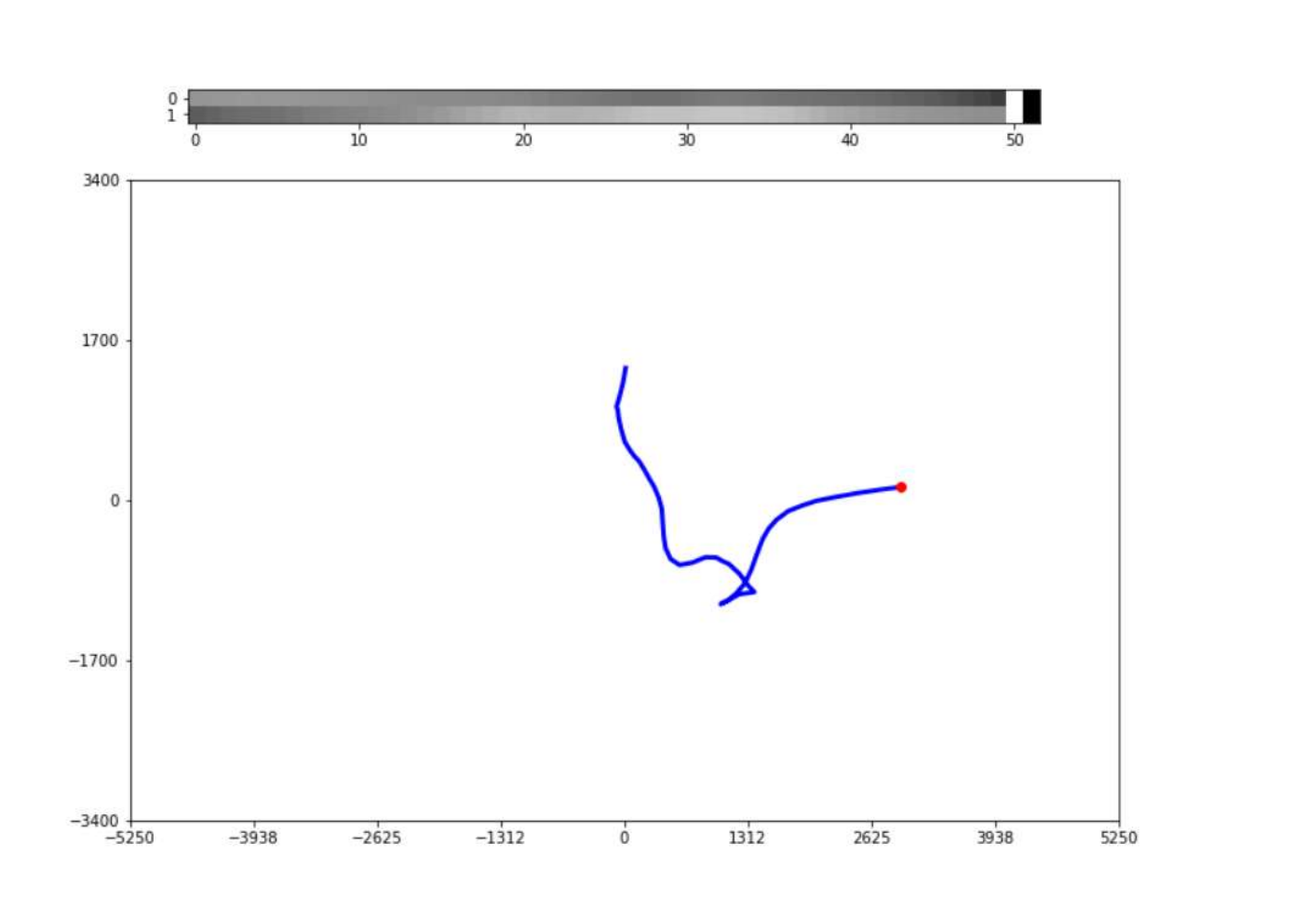
GANs have been used with great success in image recognition, 3D-models reconstruction and photorealistic imaging; see e.g. Karazeev (2017). Because of the limited time available to us, we decided to capitalize on existing codes for images; we use Bruner and Deshpande (2017). By rescaling the data accordingly we map the football field to the square $[-1,1]^{2}$ and interpret a $10$ seconds trajectory as a $2\times 100$ gray-scale image: for each of the 100 time points, the two degrees of freedom indicate the rescaled $x$- and $y$-positions. This “image” is what we input into the neural network machinery.

The algorithm we use is a repurposed version of the basic convolutional neural network found at Bruner and Deshpande (2017), which is meant to recognize and reproduce handwritten digits. There is a structural difference between the two:

• •

  the original algorithm works with the MNIST digit dataset, which consists of $28\times 28$ black-and-white images of $10$ possible states (the digits $0$-$9$);

• •

  our algorithm works with $2\times 100$ gray-scale images, containing an aggregation of $10$ seconds of play.

If we were to convert our gray-scale images to black-and-white, we would lose too much information.

Another important difference is in the intrinsic asymmetry of the data:

• •

  in the original version, both the Discriminator and the Generator look at $3\times 3$ or $5\times 5$ spatial features of the images: useful information about the topology of the shape can be obtained by looking at spatial neighborhoods of any given pixel;

• •

  in our case we want to look a the $x$ and $y$ coordinates independently, therefore our Discriminator and Generator work with one-dimensional temporal features: the information regarding the $x$- or $y$-trajectory in a temporal neighborhood of each position, i.e., its recent past and future. The information about the recent past and future of the trajectory should not be too small, otherwise the feature only observes the position of a player. On the other hand, if the feature is too large, it observes almost the entire 10-second trajectory, and the trajectory only contains a few features. To balance this trade-off we use $1\times 5$ and $1\times 10$ temporal features.

By making this tweak to the original algorithm we exploit the natural directionality of the data and we avoid overlapping the spatial properties (i.e., the shade of gray) and the temporal properties (i.e., the variation in shade). To have a sense of what this means we visualize the correspondence between the $(x,y)$-coordinates and the real trajectory of a player, see Figure 7.

We limit our training set to all random samplings of 20-second trajectories of any single player (excluding goalkeepers and the ball) during a single fixed match. This should give some extra structure for the network to work with while maintaining a diverse enough data sample.

The initialization of the parameters is the same as in the original algorithm, the Generator takes a standard Gaussian noise vector as input and then produces a new image based on the updates made by the network. To have a glance of what an untrained Generator is capable of, see Figure 8.

The Discriminator is then pre-trained with real and generated trajectories. After this first training epoch, the Discriminator is able to correctly discriminate between the real trajectories and the untrained noisy ones produced by the Generator. Here an epoch consists of one full learning cycle on the training set. Then the main training session begins. From the second epoch and above, the Discriminator is trained with real and generated data and the Generator itself is trained against the Discriminator. This produces a Generator-Discriminator feedback loop that forces both networks to improve themselves with the objective to outperform the other. This is achieved by implementing a loss function to measure three quantities:

• •

  Discriminator loss vs real: it measures how far the Discriminator is from labeling a real trajectory as “realistic”;

• •

  Discriminator loss vs Generator: it measures how far the Discriminator is from labeling a generated image as “fake”;

• •

  Generator loss vs Discriminator: it measures how far the Discriminator is from labeling a generated image as “realistic”.

The first loss function deals with the interaction between the Discriminator and the real world, it makes sure that the network is adapting to recognize new real observations. The second and third loss functions on the other hand, work against each other: one is trying to force the Discriminator to always label “fake” when presented with a generated image, while the other is forcing the Generator to produce data that mimics the Discriminator’s perception of the real world. The loss function used throughout the algorithm is the cross-entropy loss, for a discussion see Seita (2017).

Properly training a GAN requires a long time and much can go wrong in the process. The Generator and Discriminator need to maintain a perfect balance, otherwise one will outperform the other causing either the Discriminator to blindly reject any generated image, or the Generator to exploit blind spots the Discriminator may have. After a training session of $15$ hours our GAN managed to go from random noise trajectories to smooth and structured ones, although not fully learning the underlying structure of the data. While the generated movements look impressive when compared to the untrained ones, they are still underperforming when confronted with the real world. First and foremost, the acceleration pattern of the players make no physical sense, i.e., the algorithm is not able to filter out local small noise, and the trajectories are not smooth enough. The evolution of the network during training is shown in Figure 9. In the end the GAN is not consistent enough when asked to generate large samples of data: too many trajectories do not look realistic.

In parallel, we implemented a Variational Autoencoder (VAE) as introduced by Kingma and Welling (2013). Like a GAN, a VAE is an unsupervised machine-learning algorithm that gives rise to a generative model.

We will apply the VAE algorithm on normalized trajectory data spanning 50 seconds. We call the set of all such trajectory data $X$. As the trajectories are sampled at intervals of 0.1 seconds, this means that we can identify $X$ with $[0,1]^{1000}$.

A VAE consists of two neural networks, an encoder and a decoder. The encoder is a function (parametrized by a vector $\phi$)

that maps from the product of the space $X$ of input data and a space of noise variables $\mathcal{E}$, to the so-called latent space $Z$. We identify the space $Z$ with $\mathbb{R}^{d}$ ($d=10$). The decoder is a function (parametrized by a vector $\theta$)

which maps from the latent space $Z$ and a second space of noise variables $\Omega$ back to the data space $X$.

We choose the spaces of noise variables $\mathcal{E}$ and $\Omega$ to be Euclidean, with the same dimension as $Z$ and $X$ respectively, and endow them with standard Gaussian measures.

The encoder and decoder have a special structure. We implemented (as neural networks) functions

and chose

Here, $\mathrm{diag}(\sigma_{Z,\phi}(x))$ is a diagonal matrix with $\sigma_{Z,\phi}(x)$ on the diagonal. Equivalently, $\mathrm{diag}(\sigma_{Z,\phi}(x))\epsilon$ is just the elementwise product of $\sigma_{Z,\phi}(x)$ and $\epsilon$.

Similarly, we implemented a function

and selected a constant $\sigma_{X}\in(0,\infty)$ and chose

The decoder provides us with a generative model for the data: to generate a data point we first sample $z$ and $\omega$ independently according to standard normal distributions, after which we apply the decoder to the pair $(z,\omega)$. Alternatively, we can generate zero-noise samples by only sampling $z$ and computing $\mathsf{Dec}_{\theta}(z,0)$.

The Variational Autoencoder $\mathsf{VAE}_{\phi,\theta}:X\times\mathcal{E}\times\Omega\to X$ is the composition of the encoder and decoder in the sense that

The parameters $\phi$ and $\theta$ of the VAE are optimized simultaneously, so that when we apply the VAE to a randomly selected triple of trajectory $x$, noise variable $\epsilon$ and noise variable $\omega$, the result is close to the original trajectory, at least on average.

To this end, we follow Kingma and Welling (2013) and minimize an average loss, for the loss function $\mathcal{L}_{\phi,\theta}:X\times\mathcal{E}\to\mathbb{R}$ given by

For a derivation of this loss function, we refer the reader to the Appendix.

We implemented the Autoencoder in the Keras library for Python (Chollet et al., 2015). The library comes with an example VAE which we took as a starting point. We introduced a hidden layer $H_{E}$ in the encoder and $H_{D}$ in the decoder, which we both identified with $\mathbb{R}^{400}$, and implemented the functions $\mu_{Z,\phi}$ and $\sigma_{Z,\phi}$ as

where $h_{E,\phi}:X\to H_{E}$ is the composition of an affine map and ReLu activation functions, the functions $m_{Z,\phi},{l}_{Z,\phi}:H_{E}\to Z$ are linear and $\exp:Z\to Z$ is the exponential function applied componentwise.

Similarly,

where the function $h_{D,\theta}:Z\to H_{D}$ is again a composition of an affine map and ReLu activation functions and the function $m_{X,\theta}:H_{D}\to X$ is a composition of an affine map and sigmoid activation functions.

We trained the model, i.e. we adjusted the parameters $\phi$ and $\theta$ to minimize the average loss, using the ‘rmsprop’ optimizer in its default settings. Whether the model trained successfully or not did seem to depend crucially on the version of the libraries used. For the results presented below, we used Keras version 2.1.3 on top of Theano version 1.0.1. We first set $\sigma_{X}\approx 0.15$. After training for 1000 epochs, the average loss was slightly below $2$.

We used the VAE to approximate trajectories. We sampled at random trajectories $x_{i}$ from the data, and compared them to their approximations

The average absolute deviation per coordinate per time-step (expressed as a ratio with respect to the dimensions of the playing field) was approximately $0.02$, the average squared error per coordinate per time step was approximately $0.0008$ and the average maximum error per coordinate, taken over the whole trajectory, was less than $0.09$.

In Figure 10 we show the result of sampling four random trajectories $x_{i}$ from the data, and comparing them to their approximation by the VAE. The approximating trajectories are much smoother than the original ones. Some qualitative features of the original paths, such as turns and loops, are also present in the approximating paths. Even though the average error in the distance per coordinate per time step is relatively small, visually there is still quite some deviation between the true and the approximating trajectories. We expect, however, that with a more extensive network, consisting of more convolutional layers, we can greatly improve the approximation.

Next, we use the decoder of the VAE as a generative model. In particular, we sample trajectories in $X$ at random by first sampling $z\in Z$ according to a standard normal distributions, and computing the trajectory $\mathsf{Dec}_{\theta}(z,0)$. A collection of six trajectories generated in this way is shown in Figure 11. At first sight, the generated trajectories look like they could have been real trajectories of football players. However, they are in general smoother than the real trajectories. We could also have generated trajectories by sampling both $z$ and $\omega$ according to standard normal distributions and computing $\mathsf{Dec}_{\theta}(z,\omega)$. However, those trajectories would have been much too noisy.

If we reduce the value of $\sigma_{X}$ to approximately $0.008$ and retrain the model, the approximation of the trajectories becomes slightly better, and the final average loss reduces to 0.67 after training for 600 epochs. The corresponding plots look similar to Figure 10. However, if we now use the decoder to generate trajectories, most of the trajectories end up close to the boundary of the playing field: the dynamics of the generated trajectories is then clearly very different from the original dynamics.

In Appendix A, we explain this effect by investigating the different parts of the loss function given in (4.1). The upshot is that when $\sigma_{X}$ is very small, the proportion of latent variables $z\in Z$ that are in the range of the encoder is very small (measured with the Gaussian measure on $Z$). If one applies the decoder to a $z\in Z$ which is in the range of the encoder, one probably gets a realistic trajectory. But for latent variables $z$ not in the range of the encoder, there is no reason for the decoded trajectories to look realistic at all.

In the previous sections, we studied several methods to create generative models for the movement trajectories of football players, with the aim of capturing the underlying dynamics and statistics. In this section, we study to what extent movement trajectories of different soccer players can be distinguished. To this end, we test the Discriminator network of the GAN introduced in Section 4.1 on data of different soccer players. We train the Discriminator on the data of two soccer players, and then test if the Discriminator is able to distinguish their motion patterns. The success rate of the Discriminator to distinguish one player from the other then gives some insight in how different are the movement behaviors of two different players.

The loss function for the Discriminator is the same as in Section 4.1. The data we use as input for the Discriminator are $(x,y)$-coordinates of 10-second player trajectories. We test the Discriminator on these unedited $(x,y)$-trajectories, and on centered $(x,y)$-trajectories, where the coordinates of each trajectory are centered such that the first coordinate always equals $(0,0)$. Thus, by using the uncentered data, the Discriminator may distinguish two players by using their positions on the field, whereas the Discriminator can only use movement patterns of particular players when the centered data are used.

Figure 12 shows the Discriminator loss function for both players as a function of the number of training steps for two different sets of two players. We see that the loss function declines more for the uncentered data than for the centered data. Thus, the Discriminator distinguishes uncentered trajectories based on the location on the field where the movement pattern happens. The two different examples also show that it is easier to distinguish some players than others.

Table 1 shows the success rate of correctly identifying the player corresponding to a given trajectory after the training period for the two sets of players of Figure 12. The success rate of the Discriminator using the uncentered data is higher than for the centered data in both examples. Using the centered data, the Discriminator has difficulties distinguishing between players 1 and 2 in the first example. In the second example, the success rate is much higher. Thus, some players display more similarities in their movement patterns than other players.

References

- Bruner and Deshpande (2017) J. Bruner and A. Deshpande. Generative adversarial networks for beginners. Retrieved from https://www.oreilly.com/learning/generative-adversarial-networks-for-beginners, 2017.
- Chollet et al. (2015) F. Chollet et al. Keras. https://keras.io, 2015.
- Goff and Carré (2009) J. E. Goff and M. J. Carré. Trajectory analysis of a soccer ball. American Journal of Physics, 77(11):1020–1027, 2009.
- Goodfellow et al. (2014) I. Goodfellow, J. Pouget-Abadie, M. Mirza, B. Xu, D. Warde-Farley, S. Ozair, A. Courville, and Y. Bengio. Generative adversarial nets. In Advances in Neural Information Processing Systems 27, pages 2672–2680. 2014.
- Helske (2017) J. Helske. KFAS: Exponential family state space models in R. Journal of Statistical Software, 78(10):1–39, 2017.
- Karazeev (2017) A. Karazeev. Generative adversarial networks (GANs): Engine and applications. Retrieved from https://blog.statsbot.co/generative-adversarial-networks-gans-engine-and-applications-f96291965b47, 2017.
- Kingma and Welling (2013) D. P. Kingma and M. Welling. Auto-Encoding Variational Bayes. arXiv:1312.6114, 2013.
- Koopman and Durbin (2000) S. J. Koopman and J. Durbin. Fast filtering and smoothing for multivariate state space models. Journal of Time Series Analysis, 21(3):281–296, 2000.
- Koopman and Durbin (2003) S. J. Koopman and J. Durbin. Filtering and smoothing of state vector for diffuse state-space models. Journal of Time Series Analysis, 24(1):85–98, 2003.
- Ren et al. (2008) J. Ren, J. Orwell, G. A. Jones, and M. Xu. Real-time modeling of 3-d soccer ball trajectories from multiple fixed cameras. IEEE Transactions on Circuits and Systems for Video Technology, 18(3):350–362, 2008.
- Seita (2017) D. Seita. Understanding generative adversarial networks. Retrieved from https://danieltakeshi.github.io/2017/03/05/understanding-generative-adversarial-networks/, 2017.
- Yu et al. (2003a) X. Yu, Q. Tian, and K. W. Wan. A novel ball detection framework for real soccer video. In International Conference on Multimedia and Expo, 2003. ICME ’03. Proceedings., pages II–265–8 vol.2, 2003a.
- Yu et al. (2003b) X. Yu, C. Xu, Q. Tian, and H. W. Leong. A ball tracking framework for broadcast soccer video. In 2003 International Conference on Multimedia and Expo. ICME 03. Proceedings (Cat. No.03TH8698). IEEE, 2003b. doi: 10.1109/icme.2003.1221606.