跳到论文正文
W Papers独立论文阅读器 arXiv:1808.04523 论文正文 计算阅读时间 · 0%
引用这篇论文根据当前论文元数据生成,正式投稿前建议核对。


License: arXiv.org perpetual non-exclusive license
arXiv:1808.04523v3 [cs.LG] 26 Aug 2018

Adaptive Sampling for Convex Regression

Max Simchowitz ††thanks: UC Berkeley, CA. msimchow@berkeley.edu.    Kevin Jamieson ††thanks: University of Washington, WA. jamieson@cs.washington.edu    Jordan W. Suchow ††thanks: UC Berkeley, CA. suchow@berkeley.edu.    Thomas L. Griffiths ††thanks: UC Berkeley, CA. tom_griffiths@berkeley.edu
Abstract

In this paper, we introduce the first principled adaptive-sampling procedure for learning a convex function in the L∞L_{\infty} norm, a problem that arises often in the behavioral and social sciences. We present a function-specific measure of complexity and use it to prove that, for each convex function f⋆f_{\star}, our algorithm nearly attains the information-theoretically optimal, function-specific error rate. We also corroborate our theoretical contributions with numerical experiments, finding that our method substantially outperforms passive, uniform sampling for favorable synthetic and data-derived functions in low-noise settings with large sampling budgets. Our results also suggest an idealized “oracle strategy”, which we use to gauge the potential advance of any adaptive-sampling strategy over passive sampling, for any given convex function.

1 Introduction

Many functions that model individual economic utility, the output of manufacturing processes, and natural phenomena in the social sciences are either convex or concave. For example, convex functions are used to model utility functions that exhibit temporal discounting, a classic effect in behavioral economics where people value immediate rewards over delayed rewards (Frederick et al., 2002; Green and Myerson, 2004). To measure such curves, it is common practice to manipulate a variable (e.g., delay) over a fixed, uniformly spaced grid of ≈\approx design points 5 points (Fisher, 1937), collect many repeated trials of data, and fit a function of assumed parametric form (e.g., exponential or hyperbolic) using maximum likelihood estimation. This approach can be brittle to model mismatch when the true function ff lies outside the assumed class of functions. Moreover, non-linear parametric families can introduce challenges for constructing faithful and accurate confidence intervals when interpolating the estimator between measured design points.

Non-parametric convex regression (c.f. Dümbgen et al. (2004)) corrects for the shortcomings of parametric methods by making no assumptions other than that ff is convex. In additional to faithfully modeling a large class of functions, non-parametric methods can also be employed to construct error bars at any x∈[0,1]x\in[0,1] (see Cai et al. (2013)). Unfortunately, even with shape restrictions, non-parametric methods may require prohibitively many samples for practical use.

In this paper, we propose a more parsimonious approach to non-parametric curve estimation by allowing the design points to be chosen sequentially and adaptively. Formally, we consider the problem of estimating an unknown convex function f⋆:[0,1]→ℝf_{\star}:[0,1]\to\mathbb{R} with an estimator f^\widehat{f} which is close in the L∞L_{\infty} metric ‖f^−f∗‖∞=supx|f⋆​(x)−f^​(x)|\|\widehat{f}-f^{*}\|_{\infty}=\sup_{x}|f_{\star}(x)-\widehat{f}(x)| . The estimator is constructed from sequential, noisy evaluations y1,…,y𝝉y_{1},\dots,y_{\bm{\tau}} from an oracle FF at design points x1,…,x𝝉x_{1},\dots,x_{\bm{\tau}},

yt=F⁡(xt),where ​F​(xt)=f⋆​(xt)+wt,\displaystyle y_{t}=F(x_{t}),~\text{where }F(x_{t})=f_{\star}(x_{t})+w_{t}, (1)

and where wtw_{t} represents zero-mean noise. We let ℱt\mathcal{F}_{t} denote the filtration generated by the design points and measurements (xs,ys)s=1t(x_{s},y_{s})_{s=1}^{t} up to time tt, and assume that the number of samples 𝝉\bm{\tau} is a stopping time with respect to {ℱt}\{\mathcal{F}_{t}\}, where wt|ℱt−1w_{t}\big|\mathcal{F}_{t-1} is zero mean, σ2\sigma^{2}-subgaussian. We refer to measurement allocation strategies for which xt+1x_{t+1} does not depend on (xs,ys)s=1t(x_{s},y_{s})_{s=1}^{t} as passive, and adaptive sampling strategies for which xt+1x_{t+1} may depend on (xs,ys)s=1t(x_{s},y_{s})_{s=1}^{t} as active.

Our main contributions are the following:

  • •

    Inspired by Cai et al. (2013), we introduce the local approximation modulus, a new measure of local curvature for convex functions, ω⁡(f⋆,x,ϵ)\omega(f_{\star},x,\epsilon), and a function-specific complexity measure Λavg​(f⋆,ϵ)≈∫01ω​(f⋆,x,ϵ)−1​𝑑x\Lambda_{\mathrm{avg}}(f_{\star},\epsilon)\approx\int_{0}^{1}\omega(f_{\star},x,\epsilon)^{-1}dx, called the average approximation modulus. Λavg​(f⋆,ϵ)\Lambda_{\mathrm{avg}}(f_{\star},\epsilon) coincides with the average curvature of f⋆f_{\star}, up to logarithmic factors and endpoint considerations. We prove a function-specific lower bound on the sample complexity of actively estimating any convex function f⋆f_{\star} to L∞L_{\infty}-error ϵ\epsilon that scales at least as (1+σ2ϵ2)​Λavg​(f⋆,ϵ)(1+\frac{\sigma^{2}}{\epsilon^{2}})~\Lambda_{\mathrm{avg}}(f_{\star},\epsilon), up to logarithmic factors.

  • •

    The packing argument for constructing our lower bound explicitly describes a near-optimal, clairvoyant sampling allocation tailored to f⋆f_{\star}; we call this the “oracle allocation” (Proposition 3.4). This allocation is instructive as an experimental benchmark when f⋆f_{\star} is known.

  • •

    We introduce an active sampling procedure and an estimator f^\widehat{f} whose sample complexity for any particular f∗f^{*} scales as (1+σ2ϵ2)⋅Λavg​(f⋆,ϵ)(1+\frac{\sigma^{2}}{\epsilon^{2}})\cdot\Lambda_{\mathrm{avg}}(f_{\star},\epsilon) up to logarithmic factors, nearly matching our lower bounds.

  • •

    We show that for passive designs (e.g., sampled evenly on a grid), the sample complexity necessarily scales as (1+σ2ϵ2)⋅Λmax​(f,ϵ)(1+\frac{\sigma^{2}}{\epsilon^{2}})\cdot\Lambda_{\mathrm{max}}(f,\epsilon), where Λmax​(f,ϵ)≈maxx∈[0,1]⁡ω⁡(f⋆,x,ϵ)\Lambda_{\mathrm{max}}(f,\epsilon)\approx\max_{x\in[0,1]}\omega(f_{\star},x,\epsilon) coincides with the ​m​a​x​i​m​u​m\emph{maximum} curvature. We compare Λavg​(f⋆,ϵ)\Lambda_{\mathrm{avg}}(f_{\star},\epsilon) and Λmax​(f⋆,ϵ)\Lambda_{\mathrm{max}}(f_{\star},\epsilon) for many natural classes of functions, including quadratic functions, exponential curves, and kk-piecewise linear functions. For kk-piecewise linear functions, the L∞L_{\infty} error of our active algorithm scales no slower than kn−1/2lognkn^{-1/2}\log n, whereas passive designs scale no faster than n−1/3n^{-1/3} after nn evaluations (see Remark 3.2).

Finally, we validate our theoretical claims with an empirical study using both synthetic functions and those derived from real data. We observe that in low-noise settings or when the sampling budget is large, active sampling can substantially outperform passive uniform sampling. Moreover, our algorithm constitutes the first theoretically justified algorithm (passive or active) that guarantees uniform accuracy, even at the boundaries of the interval (Cai et al., 2013; Dümbgen et al., 2004). Even so, comparing the performance of our active algorithm to the oracle sampling strategy suggests room for modest but non-negligible improvements.

1.1 Related Work

Castro et al. (2005) and Korostelev (1999) studied the minimax rates of active non-parametric regression, showing that active and passive learning attain the same minimax rates of convergence for Holder smooth classes, but that active learning achieves faster rates when the function is known to be well approximated by a piecewise-constant function.

Prior literature on convex and concave regression consider the passive design case, where the design points do not depend on measurements. Typically, the design points are chosen to be uniformly spaced on the unit interval, that is, xi=1n−1x_{i}=\frac{1}{n-1} for i=0,…,n−1i=0,\dots,n-1 (Dümbgen et al., 2004). If ℱ\mathcal{F} is the set of Lipschitz, convex functions, then the L∞L_{\infty}-norm ‖f^LS−f⋆‖L∞=supx∈[0,1]|f⋆​(x)−f^LS​(x)|\|\widehat{f}_{\mathrm{LS}}-f_{\star}\|_{L_{\infty}}=\sup_{x\in[0,1]}|f_{\star}(x)-\widehat{f}_{\mathrm{LS}}(x)| of the least squares estimator f^LS\widehat{f}_{\mathrm{LS}} decreases like (log⁡(n)/n)1/3(\log(n)/n)^{1/3}, whereas if the convex function has Lipschitz gradients, the rate improves to (log⁡(n)/n)2/5(\log(n)/n)^{2/5} (Dümbgen et al., 2004).

Recent work by Guntuboyina and Sen (2015) and Chatterjee (2016) has aimed at developing sharp errors bounds on the squared L2L_{2}-norm ‖f^−f⋆‖L22:=∫x∈[0,1]|f^​(x)−f⋆​(x)|2​𝑑x\|\widehat{f}-f_{\star}\|_{L_{2}}^{2}:=\int_{x\in[0,1]}|\widehat{f}(x)-f_{\star}(x)|^{2}dx of the least squares estimator, when samples are uniformly spaced on a grid. They show that even with this uniform allocation, the error ‖f^−f⋆‖L22\|\widehat{f}-f_{\star}\|_{L_{2}}^{2} adapts to the true regression functions f⋆f_{\star}. For example, Chatterjee (2016) and Bellec et al. (2018) show that if f⋆f_{\star} is a kk-piecewise linear function, then f^LS\widehat{f}_{\mathrm{LS}} obtains the parametric error rate of ‖f^LS−f⋆‖L22≤C​k/n\|\widehat{f}_{\mathrm{LS}}-f_{\star}\|_{L_{2}}^{2}\leq Ck/n. In a similar vein, Cai et al. (2013) proves sharp confidence intervals for f⋆​(x0)f_{\star}(x_{0}) for a fixed point x0∈(0,1)x_{0}\in(0,1).

Our work draws heavily upon Cai et al. (2013) (who in turn build on Dümbgen et al. (2003)), whose aim was to characterize the function-specific sample complexity of estimating a convex ff at a given point in the interior of [0,1][0,1], from uniform measurements. We extend these tools to characterize the complexity of estimating ff with uniform accuracy over the interval [0,1][0,1], from measurements which may be chosen in an adaptive, function-dependent manner. We are thus able to obtain exceptionally granular, instance-specific results similar to those in the multi-arm bandit literature (Kaufmann et al., 2016), and in recent work studying the local minimax sample complexity of convex optimization (Zhu et al., 2016).

2 Efficiently Learning a Convex Function

We begin by establishing preliminary notation. The class of convex functions is denoted as ℱconv:={f:[0,1]→ℝ|f((1−λ)x+λy)≤(1−λ)f(x)+λf(y),∀x,y,λ∈[0,1]}\mathcal{F}_{\mathrm{conv}}:=\{f:[0,1]\to\mathbb{R}|f((1-\lambda)x+\lambda y)\leq(1-\lambda)f(x)+\lambda f(y),~\forall x,y,\lambda\in[0,1]\}. For an interval I=[a,b]⊆[0,1]I=[a,b]\subseteq[0,1], define the left-, middle- and right-endpoints as xl⁡(I)=a,xm⁡(I)=a+b2,xr⁡(I)=bx_{l(I)}=a,x_{m(I)}=\frac{a+b}{2},x_{r(I)}=b. We define the secant approximation of ff on an interval I⊂[0,1]I\subset[0,1] as

Sec⁡[f,I]​(x)=xr⁡(I)−xxr⁡(I)−xl⁡(I)​f​(xl⁡(I))+x−xl⁡(I)xr⁡(I)−xl⁡(I)​f​(xr⁡(I)),\displaystyle\mathrm{Sec}[f,I](x)=\frac{x_{r(I)}-x}{x_{r(I)}-x_{l(I)}}f(x_{l(I)})+\frac{x-x_{l(I)}}{x_{r(I)}-x_{l(I)}}f(x_{r(I)})~, (2)

and note that for a convex function, this approximation never underestimates ff; that is, one has Sec⁡[f,I]​(x)≥f⁡(x)\mathrm{Sec}[f,I](x)\geq f(x). We denote the error of the second approximation to ff on II at the midpoint xmx_{m} as

Δ⁡(f,I):=Sec⁡[f,I]​(xm⁡(I))−f⁡(xm⁡(I))=f⁡(xl⁡(I))+f⁡(xr⁡(I))2−f⁡(xm⁡(I)).\displaystyle\Delta(f,I):=\mathrm{Sec}[f,I](x_{m(I)})-f(x_{m(I)})=\frac{f(x_{l(I)})+f(x_{r(I)})}{2}-f(x_{m(I)})~.

In addition, we overload notation so that for any x,tx,t such that x∈[t,1−t]x\in[t,1-t], we have Δ⁡(f,x,t):=Δ⁡(f,[x−t,x+t])\Delta(f,x,t):=\Delta(f,[x-t,x+t]).

We now state a remarkable fact about convex functions that is at the core of our analysis.

Lemma 2.1

For convex ff, Δ⁡(f,I)≤maxx∈I⁡{Sec⁡[f,I]​(x)−f⁡(x)}≤2​Δ​(f,I)\displaystyle\Delta(f,I)\leq\max_{x\in I}\left\{\mathrm{Sec}[f,I](x)-f(x)\right\}\leq 2\Delta(f,I).

Lemma 2.1 is a special case of a more general lemma stated in Section 6 that upper bounds the supremum of the secant approximation error by a constant using only a single point within the interval. Convexity is critical to the proof of this lemma and such a property does not hold, for instance, on merely monotonic functions. We remark that the first inequality is trivial, and the second inequality is tight in the sense that it is achieved by f⁡(x)=(1−x)pf(x)=(1-x)^{p} on interval I=[0,1]I=[0,1] as p→∞p\rightarrow\infty.

The above observations motivate our strategy of approximating ff with secant approximations on disjoint intervals whose union is [0,1][0,1]. The next definition relates the secant approximation error to the required sampling density.

Definition 1 (Local Approximation Modulus)

We define the ϵ\epsilon-approximation modulus of ff at a point x∈[0,1]x\in[0,1] as the least tt such that the midpoint secant approximation to ff on [x−t,x+t][x-t,x+t] has bias ϵ\epsilon:

ω⁡(f,x,ϵ):=min⁡{t∈[0,min⁡{x,1−x}]:Δ⁡(f,x,t)≥ϵ}.\displaystyle\omega(f,x,\epsilon):=\min\left\{t\in\left[0,\min\left\{x,1-x\right\}\right]:\Delta\left(f,x,t\right)\geq\epsilon\right\}. (3)

Note that ω⁡(f,x,ϵ)>0\omega(f,x,\epsilon)>0 for all x∈(0,1)x\in(0,1), because convex functions are continuous on their domain. Intuitively, ω⁡(f,x,ϵ)\omega(f,x,\epsilon) is the scale at which ff “looks” linear around some xx, up to a tolerance ϵ\epsilon. Away from the endpoints {0,1}\{0,1\}, smaller values of ω⁡(f,x,ϵ)\omega(f,x,\epsilon) correspond to larger complexities, because they imply that ff can only be approximated by a linear function on a small interval. But if xx is the near {0,1}\{0,1\}, ω⁡(f,x,ϵ)≤min⁡{x,1−x}\omega(f,x,\epsilon)\leq\min\{x,1-x\} will take small values, potentially overestimating the local complexity. We remedy this issue by defining the following left- and right-approximation points:

tleft​(f,ϵ)\displaystyle t_{\mathrm{left}}(f,\epsilon) :=inf{t≤1/2:Δ⁡(f,t,t)≥ϵ}\displaystyle:=\inf\left\{t\leq 1/2:\Delta\left(f,t,t\right)\geq\epsilon\right\}
tright​(f,ϵ)\displaystyle t_{\mathrm{right}}(f,\epsilon) =inf{t≤1/2:Δ⁡(f,1−t,t)≥ϵ}.\displaystyle=\inf\left\{t\leq 1/2:\Delta\left(f,1-t,t\right)\geq\epsilon\right\}\,.

Within [tleft​(f,ϵ),1−tright​(ϵ)][t_{\mathrm{left}}(f,\epsilon),1-t_{\mathrm{right}}(\epsilon)], we will show that the midpoint errors Δ⁡(f,x,t)\Delta(f,x,t) concisely describe how densely one would need to sample ff in the neighborhood of x∈[0,1]x\in[0,1] in order to estimate it to the desired accuracy ϵ\epsilon in the L∞L_{\infty}-norm. Moreover, we show that it suffices to sample at constant number of design points on the end-intervals [0,tleft​(f,ϵ)][0,t_{\mathrm{left}}(f,\epsilon)] and [1−tright​(ϵ),1][1-t_{\mathrm{right}}(\epsilon),1]. At a high level, the main finding of this paper is as follows:

The sample complexity of learning a particular convex function f⋆f_{\star} up to ϵ\epsilon accuracy in L∞L_{\infty} with passive sampling is parametrized by the worst-case approximation modulus

Λmax​(f⋆,ϵ):=1+supx∈[tleft​(f⋆,ϵ),1−tright​(f,ϵ)]ω​(f⋆,x,ϵ)−1.\displaystyle\Lambda_{\mathrm{max}}(f_{\star},\epsilon):=1+\sup_{x\in[t_{\mathrm{left}}(f_{\star},\epsilon),1-t_{\mathrm{right}}(f,\epsilon)]}\omega(f_{\star},x,\epsilon)^{-1}. (4)

In contrast, the sample complexity of active sampling algorithms is parametrized by the average approximation modulus

Λavg​(f⋆,ϵ):=1+∫tleft​(f⋆,ϵ)1−tright​(f⋆,ϵ)ω​(f⋆,x,ϵ)−1​𝑑x.\displaystyle\Lambda_{\mathrm{avg}}(f_{\star},\epsilon):=1+\int_{t_{\mathrm{left}}(f_{\star},\epsilon)}^{1-t_{\mathrm{right}}(f_{\star},\epsilon)}\omega(f_{\star},x,\epsilon)^{-1}dx~. (5)

We emphasize that the algorithm presented in in this work guarantees accuracy on the whole interval [0,1][0,1], whereas many passive algorithms pointwise and L∞L_{\infty} risk bounds (Cai et al., 2013; Dümbgen et al., 2004) only guarantee accuracy on a strictly smaller sub-interval.

2.1 Examples

Explicit parameterizations of f⋆f_{\star} provide intuition for when active sampling is advantageous. In this section, we describe different scalings of Λmax\Lambda_{\mathrm{max}} and Λavg\Lambda_{\mathrm{avg}} for various f⋆f_{\star}; later, in Remark 3.2, we explain how these scalings can imply substantial differences in sample complexity.

2.1.1 Piecewise Linear Functions

Let f⋆f_{\star} be a Lipschitz, piecewise linear convex function with a constant number of pieces. It follows that ω​(f⋆,x,ϵ)−1≈min⁡{1ϵ,1d⁡(x,f⋆)}\omega(f_{\star},x,\epsilon)^{-1}\approx\min\{\tfrac{1}{\epsilon},\tfrac{1}{d(x,f_{\star})}\} where d⁡(x,f⋆)d(x,f_{\star}) is the distance to the closest knot adjoining any two linear pieces of f⋆f_{\star}. It follows that Λmax​(f,ϵ)≈ϵ−1\Lambda_{\mathrm{max}}(f,\epsilon)\approx\epsilon^{-1} whereas Λavg​(f,ϵ)≈log⁡(1/ϵ)\Lambda_{\mathrm{avg}}(f,\epsilon)\approx\log(1/\epsilon).

2.1.2 Bounded third-derivative:

Suppose supx∈[0,1]f⋆′′′​(x)<∞\sup_{x\in[0,1]}f_{\star}^{\prime\prime\prime}(x)<\infty. We may apply a Taylor series to find ω​(f⋆,x,ϵ)−1=f⋆′′​(x)/2​ϵ\omega(f_{\star},x,\epsilon)^{-1}=\sqrt{f_{\star}^{\prime\prime}(x)/2\epsilon} as ϵ→0\epsilon\rightarrow 0, which makes an explicit connection between the curvature of the function and the differences between Λavg​(f⋆,ϵ)\Lambda_{\mathrm{avg}}(f_{\star},\epsilon) and Λmax​(f⋆,ϵ)\Lambda_{\mathrm{max}}(f_{\star},\epsilon). This suggests that if the function has areas of high but localized curvature such as f⋆​(x)=1−xf_{\star}(x)=1-\sqrt{x} or f⋆​(x)=1100​log⁡(1+exp⁡(−100​(x−12)))f_{\star}(x)=\frac{1}{100}\log(1+\exp(-100(x-\frac{1}{2}))) then the difference between Λavg​(f⋆,ϵ)\Lambda_{\mathrm{avg}}(f_{\star},\epsilon) and Λmax​(f⋆,ϵ)\Lambda_{\mathrm{max}}(f_{\star},\epsilon) can be as vast as log⁡(1/ϵ)\log(1/\epsilon) versus 1/ϵ1/\epsilon.

2.1.3 Quadratic Functions:

Let f⋆​(x)=12​a​x2+b​x+cf_{\star}(x)=\tfrac{1}{2}ax^{2}+bx+c for some real coefficients a,b,ca,b,c. Ignoring the effect of endpoints, ω​(f⋆,x,ϵ)−1=a2​ϵ\omega(f_{\star},x,\epsilon)^{-1}=\sqrt{\frac{a}{2\epsilon}} for all xx due to the function having constant curvature, so Λavg​(f⋆,ϵ)=Λmax​(f⋆,ϵ)\Lambda_{\mathrm{avg}}(f_{\star},\epsilon)=\Lambda_{\mathrm{max}}(f_{\star},\epsilon).

3 Main Results

In this section, we state a formal upper bound obtained by Algorithm 2, described in Section 4. Algorithm 2 takes in a confidence parameter δ∈(0,1)\delta\in(0,1), as well as a second parameter β>0\beta>0 governing the degree to which the active sampling algorithm is ‘aggressive’; from simulations, we recommend setting β=1/2\beta=1/2. Lastly, at each round, Algorithm 2 maintains an estimator f^t∈ℱconv\widehat{f}_{t}\in\mathcal{F}_{\mathrm{conv}}, whose performance is characterized by the following theorem:

Theorem 3.1

Let C>0C>0 be a universal constant, and for f⋆∈ℱconvf_{\star}\in\mathcal{F}_{\mathrm{conv}}, δ∈(0,1/2)\delta\in(0,1/2) and β>0\beta>0, define cβ:=β/22+βc_{\beta}:=\tfrac{\beta/2}{2+\beta}, and

N¯β​(f⋆,ϵ,δ):=C​Λavg​(f⋆,cβ​ϵ)​max⁡{1,(1+β)2​σ2ϵ2}​log⁡(1δ​Λavg​(f⋆,cβ​ϵ)​log⁡(1+σ⁡(1+β)ϵ)).\displaystyle\overline{N}_{\beta}(f_{\star},\epsilon,\delta):=C\Lambda_{\mathrm{avg}}(f_{\star},c_{\beta}\epsilon)\,\max\left\{1,\tfrac{(1+\beta)^{2}\sigma^{2}}{\epsilon^{2}}\right\}\,\log\left(\frac{1}{\delta}\,\Lambda_{\mathrm{avg}}(f_{\star},c_{\beta}\epsilon)\,\log\left(1+\tfrac{\sigma(1+\beta)}{\epsilon}\right)\right)~.

Then, if Algorithm 2 is run with parameters δ\delta and β\beta, with access to an oracle (1), the estimators f^t∈ℱconv\widehat{f}_{t}\in\mathcal{F}_{\mathrm{conv}} and confidence estimates ϵt\epsilon_{t} defined in Section 4.2 satisfy the following any-time guarantee:

ℙf⋆,𝖠𝗅𝗀[∥f^t−f⋆∥∞≤ϵt≤ϵ for all t,ϵ:t≥N¯(f⋆,ϵ,β,δ)]≥1−δ.\displaystyle\mathbb{P}_{f_{\star},\mathsf{Alg}}\left[\|\widehat{f}_{t}-f_{\star}\|_{\infty}\leq\epsilon_{t}\leq\epsilon\text{ for all }t,\epsilon:t\geq\overline{N}(f_{\star},\epsilon,\beta,\delta)\right]\geq 1-\delta.

In the case of the default parameter setting β=1/2\beta=1/2, we find that, for a possibly larger universal constant C′C^{\prime},

N¯1​(f,ϵ,δ)≤C′​Λavg​(f,ϵ10)⋅max⁡{1,σ2ϵ2}⋅log⁡(1δ⋅Λavg​(f,ϵ10)⋅log⁡(1+σϵ)).\displaystyle\overline{N}_{1}(f,\epsilon,\delta)\leq C^{\prime}\Lambda_{\mathrm{avg}}\left(f,\frac{\epsilon}{10}\right)\cdot\max\left\{1,\frac{\sigma^{2}}{\epsilon^{2}}\right\}\cdot\log\left(\frac{1}{\delta}\cdot\Lambda_{\mathrm{avg}}\left(f,\frac{\epsilon}{10}\right)\cdot\log\left(1+\frac{\sigma}{\epsilon}\right)\right)~.

Up to constants and logarithmic factors, the sample complexity is dominated by the term Λavg​(f,ϵ/10)⋅max⁡{1,σ2ϵ2}\Lambda_{\mathrm{avg}}(f,\epsilon/10)\cdot\max\left\{1,\frac{\sigma^{2}}{\epsilon^{2}}\right\}. Here σ2ϵ2\frac{\sigma^{2}}{\epsilon^{2}} corresponds to the standard rate for estimating a scalar. The dependence on Λavg​(f,cβ​ϵ)\Lambda_{\mathrm{avg}}(f,c_{\beta}\epsilon) captures the number of points required to estimate ff with a discretized proxy.

To better understand why Λavg\Lambda_{\mathrm{avg}} is the appropriate quantity to consider, we now introduce a construction of local packings of ℱconv\mathcal{F}_{\mathrm{conv}}, centered at a given f∈ℱconvf\in\mathcal{F}_{\mathrm{conv}}. Recall that Δ⁡(f,I)\Delta(f,I) denotes the error of the secant approximation to ff on the midpoint xm⁡(I)x_{m(I)} of II, constructed using the endpoints xl⁡(I),xr⁡(I)x_{l(I)},x_{r(I)}. We note that if any algorithm, even an active one, does not measure ff on an interval II for which Δ⁡(f,I)≥ϵ\Delta(f,I)\geq\epsilon, then one cannot distinguish between ff and the alternative function f~I:=f⁡(x)+𝕀⁡(x∈I)​(Sec⁡[f,I]​(x)−f⁡(x))\tilde{f}_{I}:=f(x)+\mathbb{I}(x\in I)(\mathrm{Sec}[f,I](x)-f(x)). Thus, a key step to showing that Λ⁡(f,ϵ)\Lambda(f,\epsilon) approximately lower bounds the number of evaluations is to show that it approximately lower bounds the number of intervals II for which Δ⁡(f,I)≥ϵ\Delta(f,I)\geq\epsilon. This is achieved in the following theorem proved in Section 5.3:

Theorem 3.2 (Packing)

Let f∈ℱconvf\in\mathcal{F}_{\mathrm{conv}} be a convex function, ϵ>0\epsilon>0, and define

N¯​(f,ϵ)=⌈Λavg​(f,ϵ)4​(1+log⁡(ωmax​(f,ϵ)/ωmin​(f,ϵ)))−2⌉\displaystyle\underline{N}(f,\epsilon)=\lceil\frac{\Lambda_{\mathrm{avg}}(f,\epsilon)}{4(1+\log(\omega_{\max}(f,\epsilon)/\omega_{\min}(f,\epsilon)))}-2\rceil (6)

where ωmax​(f,ϵ):=maxx∈[tleft​(f,ϵ),1−tright​(f,ϵ)]⁡ω⁡(f,x,ϵ)\omega_{\max}(f,\epsilon):=\max_{x\in[t_{\mathrm{left}}(f,\epsilon),1-t_{\mathrm{right}}(f,\epsilon)]}\omega(f,x,\epsilon) and ωmin\omega_{\min} is defined analogously. Then, there is an Npck​(f,ϵ)≥N¯​(f,ϵ)N_{\mathrm{pck}}(f,\epsilon)\geq\underline{N}(f,\epsilon) such that the points {zi}i=1Npck​(f,ϵ)⊂[0,1]\{z_{i}\}_{i=1}^{N_{\mathrm{pck}}(f,\epsilon)}\subset[0,1] such that the intervals

Iiϵ:=[zi−ω⁡(zi,f,ϵ),zi+ω⁡(zi,f,ϵ)],i∈[Npck​(f,ϵ)]\displaystyle I^{\epsilon}_{i}:=[z_{i}-\omega(z_{i},f,\epsilon),z_{i}+\omega(z_{i},f,\epsilon)],~i\in[N_{\mathrm{pck}}(f,\epsilon)]

have disjoint interiors, are contained in [2​tleft​(f,ϵ),1−2​tright​(f,ϵ)][2t_{\mathrm{left}}(f,\epsilon),1-2t_{\mathrm{right}}(f,\epsilon)] and satisfy Δ⁡(f,Iiϵ)=ϵ\Delta(f,I_{i}^{\epsilon})=\epsilon. Moreover, the interval endpoints overlap so that xℓ⁡(Ii+1ϵ)=xr⁡(Iiϵ)x_{\ell(I_{i+1}^{\epsilon})}=x_{r(I_{i}^{\epsilon})}.

Note that Npck​(f,ϵ)N_{\mathrm{pck}}(f,\epsilon) corresponds to the actual size of the explict packing, and N¯​(f,ϵ)\underline{N}(f,\epsilon) is a computable lower bound on Npck​(f,ϵ)N_{\mathrm{pck}}(f,\epsilon). We now consider the class 𝒢⁡(f,ϵ)⊂ℱconv\mathcal{G}(f,\epsilon)\subset\mathcal{F}_{\mathrm{conv}} of alternative functions

𝒢f,ϵ:={f(x)+∑i=1Npck​(f,ϵ)𝖻i𝕀{x∈Iiϵ}(Sec[f,Iiϵ](x)−f(x)):𝖻∈{0,1}Npck​(f,ϵ)}.\displaystyle\mathcal{G}_{f,\epsilon}:=\Big\{f(x)+\sum_{i=1}^{N_{\mathrm{pck}}(f,\epsilon)}\mathsf{b}_{i}\mathbb{I}\{x\in I^{\epsilon}_{i}\}(\mathrm{Sec}[f,I^{\epsilon}_{i}](x)-f(x)):\mathsf{b}\in\{0,1\}^{N_{\mathrm{pck}}(f,\epsilon)}\Big\}. (7)

We observe that f∈𝒢f,ϵ⊂ℱconvf\in\mathcal{G}_{f,\epsilon}\subset\mathcal{F}_{\mathrm{conv}}, and by definition, if g1,g2∈𝒢f,ϵg_{1},g_{2}\in\mathcal{G}_{f,\epsilon} are distinct, then ‖g1−g2‖∞≥ϵ\|g_{1}-g_{2}\|_{\infty}\geq\epsilon. In particular, given any set of points {xi}i=1n⊂[0,1]\{x_{i}\}_{i=1}^{n}\subset[0,1] for n<Npck​(f,ϵ)n<N_{\mathrm{pck}}(f,\epsilon), then there exist two convex functions g1,g2g_{1},g_{2} in 𝒢f,ϵ\mathcal{G}_{f,\epsilon}, such that g1​(xi)=g2​(xi)g_{1}(x_{i})=g_{2}(x_{i}) for all ii and ‖g1−g2‖∞≥ϵ\|g_{1}-g_{2}\|_{\infty}\geq\epsilon. In Section 5.2, we formalize this argument to yield the following theorem:

Theorem 3.3

Fix an f⋆∈ℱconvf_{\star}\in\mathcal{F}_{\mathrm{conv}}, ϵ>0\epsilon>0, and δ∈(0,1/3)\delta\in(0,1/3). Let N¯​(f⋆,ϵ)\underline{N}(f_{\star},\epsilon) be as in Lemma 3.2, and let and 𝒢f,ϵ\mathcal{G}_{f,\epsilon} be as given by Equation (7). Let 𝖠𝗅𝗀\mathsf{Alg} be any active algorithm that returns an estimator f^\widehat{f} at a stopping time τ\tau, and satisfies the correctness guarantee

∀g∈𝒢f⋆,2​ϵ,ℙ𝖠𝗅𝗀,g[∥f^−g∥∞<ϵ]≥1−δ.\displaystyle\forall g\in\mathcal{G}_{f_{\star},2\epsilon},~\mathbb{P}_{\mathsf{Alg},g}[\|\widehat{f}-g\|_{\infty}<\epsilon]\geq 1-\delta. (8)

Then the stopping time τ\tau, under observations from ff, is lower bounded by

𝔼f⋆,𝖠𝗅𝗀​[τ]≳N¯​(f⋆,2​ϵ)⋅max⁡{1,σ22​ϵ2​log⁡(1/δ)},\displaystyle\mathbb{E}_{f_{\star},\mathsf{Alg}}[\tau]\gtrsim\underline{N}(f_{\star},2\epsilon)\cdot\max\left\{1,\frac{\sigma^{2}}{2\epsilon^{2}}\log(1/\delta)\right\}~,

and the average sample complexity over 𝒢f,2​ϵ\mathcal{G}_{f,2\epsilon} is at least

1|𝒢f⋆,2​ϵ|​∑g∈𝒢f⋆,2​ϵ𝔼g,𝖠𝗅𝗀​[τ]≳N¯​(f⋆,2​ϵ)⋅max⁡{1,σ22​ϵ2⋅log⁡(N¯​(f⋆,2​ϵ)/δ)}.\displaystyle\frac{1}{\left|\mathcal{G}_{f_{\star},2\epsilon}\right|}\sum_{g\in\mathcal{G}_{f_{\star},2\epsilon}}\mathbb{E}_{g,\mathsf{Alg}}[\tau]\gtrsim\underline{N}(f_{\star},2\epsilon)\cdot\max\left\{1,\frac{\sigma^{2}}{2\epsilon^{2}}\cdot\log(\underline{N}(f_{\star},2\epsilon)/\delta)\right\}. (9)

The above bounds hold when N¯​(f⋆,⋅)\underline{N}(f_{\star},\cdot) is replaced by 1∨Npck1\vee N_{\mathrm{pck}}.

Remark 3.1

The additional logarithmic factor that arises in (9) is due to the fact that estimating a function g∈𝒢f,2​ϵg\in\mathcal{G}_{f,2\epsilon} to L∞L_{\infty}-error ϵ\epsilon corresponds to correctly performing N¯​(f,2​ϵ)\underline{N}(f,2\epsilon) simultaneous hypothesis tests, regarding the value of gg on each of the intervals IiϵI_{i}^{\epsilon}. However, for any fixed g∈𝒢f,2​ϵg\in\mathcal{G}_{f,2\epsilon} (and, in particular, f=gf=g), one can devise an algorithm that does not suffer this logarithmic factor by ‘biasing’ the algorithm towards that function.

In addition to providing a lower bound, the packing of Theorem 3.2 defines a near-optimal covering as well, in the sense that it defines a sampling allocation that can be used to test the hypothesis that, for a given f⋆f_{\star}, H0:{f=f⋆}H_{0}:\{f=f_{\star}\} versus H1:‖f−f⋆‖∞=Ω⁡(ϵ)H_{1}:\|f-f_{\star}\|_{\infty}=\Omega(\epsilon). Formally, we have the following:

Proposition 3.4

For every function f⋆f_{\star}, ϵ>0\epsilon>0 and δ∈(0,1)\delta\in(0,1), there exists a

T≲(1+σ2ϵ2)⋅(1∨Npck​(f⋆,ϵ))⋅log⁡((1∨Npck​(f⋆,ϵ)/δ)CLOSE,\displaystyle T\lesssim(1+\frac{\sigma^{2}}{\epsilon^{2}})\cdot(1\vee N_{\mathrm{pck}}(f_{\star},\epsilon))\cdot\log((1\vee N_{\mathrm{pck}}(f_{\star},\epsilon)/\delta),

a deterministic sampling allocation 𝒳(pck):={x1(pck),…,xT(pck)}\mathcal{X}^{(\mathrm{pck})}:=\{x^{(\mathrm{pck})}_{1},\dots,x^{(\mathrm{pck})}_{T}\}, and a test function ψ∈{0,1}\psi\in\{0,1\} constructed from the allocation 𝒳(pck)\mathcal{X}^{(\mathrm{pck})} such that

∀f∈ℱconv:∥f−f⋆∥≥10ϵ,ℙf⋆[ψ≠0]+ℙf[ψ≠1]≤δ.\displaystyle\forall f\in\mathcal{F}_{\mathrm{conv}}:\|f-f_{\star}\|\geq 10\epsilon,\quad\mathbb{P}_{f_{\star}}[\psi\neq 0]+\mathbb{P}_{f}[\psi\neq 1]\leq\delta~.

The design 𝒳(pck)\mathcal{X}^{(\mathrm{pck})} is explicitly constructed in Section 5.3 by augmenting the Npck​(f⋆,ϵ)N_{\mathrm{pck}}(f_{\star},\epsilon)-intervals in Theorem 3.2 with at most three additional intervals to ensure coverage of all of [0,1][0,1]. Crucially, we made use of the fact that intervals IiϵI_{i}^{\epsilon} share endpoints, and have secant error Sec⁡[f⋆,Iiϵ]\mathrm{Sec}[f_{\star},I_{i}^{\epsilon}] exactly equal to ϵ\epsilon. In light of Theorem 3.3, we see that the design 𝒳(pck)\mathcal{X}^{(\mathrm{pck})} is optimal for verifying that f=f⋆f=f_{\star}, up to scaling ϵ\epsilon by constant factors. For this reason, we refer to this construction as the oracle allocation since it precisely characterizes the optimal sampling allocation taken if one knew f⋆f_{\star}. In general, this allocation may be too optimistic, since an algorithm which does not know the true f⋆f_{\star} cannot choose this allocation a fortiori.

3.1 Comparison between Upper and Lower Bounds

For the purpose of comparing upper and lower bounds, we will consider running Algorithm 2 with the setting β=1\beta=1; any constant β\beta bounded away from zero will yield qualitatively similar results. We find that the upper bound of Theorem 3.1 and lower bound of Theorem 3.3 nearly match, with the following exceptions:

  1. 1.

    The upper bound involves a doubly logarithmic factor that depends on 1+σϵ1+\frac{\sigma}{\epsilon}. This is a consequence of the law of the iterated logarithm, which Algorithm 2 uses to maintain uniform correctness of its confidence intervals over time.

  2. 2.

    Theorem 3.1 is given in terms of Λ⁡(f,ϵ/6)\Lambda(f,\epsilon/6), whereas our lower bound is stated in terms of Λ⁡(f,2​ϵ)\Lambda(f,2\epsilon). The two quantities can be related by the following proposition, proved in Section 6.4.

    Proposition 3.5

    For any 0<c≤10<c\leq 1, ϵ>0\epsilon>0 and any convex ff, ω⁡(f,x,ϵ)≥ω⁡(f,x,c​ϵ)≥c​ω​(f,x,ϵ)\omega(f,x,\epsilon)\geq\omega(f,x,c\epsilon)\geq c\omega(f,x,\epsilon) for all x∈[tleft​(f,ϵ),1−tright​(f,ϵ)]x\in[t_{\mathrm{left}}(f,\epsilon),1-t_{\mathrm{right}}(f,\epsilon)]. Moreover,

    Λ⁡(f,ϵ)+log⁡tleft​(f,ϵ)​tright​(f,ϵ)tleft​(f,c​ϵ)​tright​(f,c​ϵ)≤Λ⁡(f,c​ϵ)≤1c​{Λ⁡(f,ϵ)+log⁡tleft​(f,ϵ)​tright​(f,ϵ)tleft​(f,c​ϵ)​tright​(f,c​ϵ)}.\Lambda(f,\epsilon)+\log\frac{t_{\mathrm{left}}(f,\epsilon)t_{\mathrm{right}}(f,\epsilon)}{t_{\mathrm{left}}(f,c\epsilon)t_{\mathrm{right}}(f,c\epsilon)}~\leq~\Lambda(f,c\epsilon)~\leq~\frac{1}{c}\left\{\Lambda(f,\epsilon)+\log\frac{t_{\mathrm{left}}(f,\epsilon)t_{\mathrm{right}}(f,\epsilon)}{t_{\mathrm{left}}(f,c\epsilon)t_{\mathrm{right}}(f,c\epsilon)}\right\}.

    Hence, ignoring the contributions of the endpoints tleftt_{\mathrm{left}} and trightt_{\mathrm{right}}, rescaling ϵ\epsilon by a multiplicative constant cc changes Λ⁡(f,ϵ)\Lambda(f,\epsilon) by at most cc.

  3. 3.

    Lastly, the upper and lower bounds differs in that N¯​(f,ϵ)\underline{N}(f,\epsilon) requires dividing through by log⁡(ωmax/ωmin)\log(\omega_{\max}/\omega_{\min}). We conjecture that the lower bound more accurately reflects the true sample complexity; see Remark A.1.

3.2 Sample Complexity for Passive Designs

In this section, we show that the sample complexity for estimating a convex function ff with an approximately uniform passive design up to error ϵ\epsilon is governed by the parameter Λmax​(f)\Lambda_{\mathrm{max}}(f).

Theorem 3.6

Consider a (possibly randomized) passive design {xi}i=1n\{x_{i}\}_{i=1}^{n}, which is uniform in the sense that, for some τ>1\tau>1, and any interval I=[a,b]I=[a,b] with b−a≤1/nb-a\leq 1/n, one has that 𝔼⁡[|{xi:xi∈[a,b]}|]≤τ\mathbb{E}[|\{x_{i}:x_{i}\in[a,b]\}|]\leq\tau. Then, for a universal constant cc, any δ∈(0,1/3)\delta\in(0,1/3) and all f∈ℱconvf\in\mathcal{F}_{\mathrm{conv}} such that (1+σ2ϵ2)​Λmax​(f,2​ϵ)≥c​n​log⁡(1/δ)/τ\left(1+\frac{\sigma^{2}}{\epsilon^{2}}\right)\Lambda_{\mathrm{max}}(f,2\epsilon)~\geq cn\log(1/\delta)/\tau, there exists an alternative f~∈ℱconv\widetilde{f}\in\mathcal{F}_{\mathrm{conv}} such that

supg∈{f,f~}ℙ𝖠𝗅𝗀,g[∥f^−g∥∞≥ϵ]≥δ.\displaystyle\sup_{g\in\{f,\widetilde{f}\}}\mathbb{P}_{\mathsf{Alg},g}[\|\widehat{f}-g\|_{\infty}\geq\epsilon]\geq\delta.

The proof for the above theorem is as follows. Let

x∗:=arginf{ω(f,x,2ϵ):x∈[tleft(f,2ϵ),1−tright(f,2ϵ)]}.\displaystyle x_{*}:=\arg\inf\left\{\omega(f,x,2\epsilon):x\in[t_{\mathrm{left}}(f,2\epsilon),1-t_{\mathrm{right}}(f,2\epsilon)]\right\}.

which intuitively corresponds to the point with the highest local curvature. Further, let I∗:=[x∗−ω⁡(f,x∗,2​ϵ),x∗+ω⁡(f,x∗,2​ϵ)]I_{*}:=[x_{*}-\omega(f,x_{*},2\epsilon),x_{*}+\omega(f,x_{*},2\epsilon)], so that 1/|I∗|≳Λmax​(f,2​ϵ)1/|I_{*}|\gtrsim\Lambda_{\mathrm{max}}(f,2\epsilon). If we consider the alternative function

f~​(x):=f⁡(x)+𝕀⁡(x∈I∗)⋅(Sec⁡[f,I∗]​(x)−f⁡(x)),\displaystyle\widetilde{f}(x):=f(x)+\mathbb{I}(x\in I^{*})\cdot\left(\mathrm{Sec}[f,I^{*}](x)-f(x)\right), (10)

then by construction, f~\widetilde{f} and ff differ only on Int⁡(I∗)\mathrm{Int}(I^{*}) and ‖f~−f‖∞≥2​ϵ\|\widetilde{f}-f\|_{\infty}\geq 2\epsilon. So if 𝖠𝗅𝗀\mathsf{Alg} can estimate ff up to L∞L_{\infty}-norm error <ϵ<\epsilon, then 𝖠𝗅𝗀\mathsf{Alg} can distinguish between ff and f~\widetilde{f}. Consequently, standard information-theoretic arguments (Section 5.2) imply that any sampling algorithm must collect ≳(1+σ2ϵ2)​log⁡(1/δ)\gtrsim(1+\frac{\sigma^{2}}{\epsilon^{2}})\log(1/\delta) samples within Int⁡(I∗)\mathrm{Int}(I_{*}). Theorem 3.6 then follows by the uniformity of the sampling procedure. In the case where the design is passive but not uniform, it is possible that the design performs well on particular functions f∈ℱconvf\in\mathcal{F}_{\mathrm{conv}}. In Remark A.2, we show that nevertheless, if the design is not uniform, it will underperform on a ‘translation’ of ff.

Remark 3.2

(Piecewise linear) If ff is Lipschitz and piecewise linear with a constant number of pieces, then from Section 2.1 we have Λmax​(f,ϵ)≈ϵ−1\Lambda_{\mathrm{max}}(f,\epsilon)\approx\epsilon^{-1} whereas Λavg​(f,ϵ)≈log⁡(1/ϵ)\Lambda_{\mathrm{avg}}(f,\epsilon)\approx\log(1/\epsilon). Theorem 3.6 implies that any (ϵ,δ)(\epsilon,\delta)-correct passive sampling procedure requires ϵ−3log(/δ)\epsilon^{-3}\log(/\delta) measurements whereas Theorem 3.1 says that our active sampling procedure takes just ϵ−2​log⁡(1/ϵ)​log⁡(log⁡(ϵ−1)/δ)\epsilon^{-2}\log(1/\epsilon)\log(\log(\epsilon^{-1})/\delta). Thus, after nn total samples the L∞L_{\infty} of passive sampling decays no faster than (1n)1/3(\tfrac{1}{n})^{1/3} whereas active sampling decays like (log⁡(n)​log⁡log​(n)n)1/2(\tfrac{\log(n)\log\log(n)}{n})^{1/2}.

4 Recursive Secant Approximation

We now introduce the recursive secant approximation algorithm for learning a convex function with noise. We begin by sampling each endpoint {0,1}\{0,1\} once. Subsequently, let t=3,4,…t=3,4,\dots denote the number of samples taken, and let 𝒯t\mathcal{T}_{t} denote a binary tree of intervals contained in [0,1][0,1], where the children of an interval II are given by [xl⁡(I),xm⁡(I)][x_{l(I)},x_{m(I)}] and [xm⁡(I),xr⁡(I)][x_{m(I)},x_{r(I)}]. We let ℒ⁡(𝒯t)\mathcal{L}(\mathcal{T}_{t}) denote the set of leaves of 𝒯t\mathcal{T}_{t}. By construction, 𝒯t\mathcal{T}_{t} immediately satisfies the following properties stipulated in Lemma 4.1:

Lemma 4.1

For any t≥1t\geq 1, we have |I∩I′|=0|I\cap I^{\prime}|=0 for any I≠I′∈ℒ⁡(𝒯t)I\neq I^{\prime}\in\mathcal{L}(\mathcal{T}_{t}); ⋃I∈ℒ⁡(𝒯t)I=[0,1]\bigcup_{I\in\mathcal{L}(\mathcal{T}_{t})}I=[0,1]; and ⋃I∈ℒ⁡(𝒯t){xm⁡(I),xl⁡(I),xr⁡(I)}=⋃I∈𝒯t{xm⁡(I),xl⁡(I),xr⁡(I)}\bigcup_{I\in\mathcal{L}(\mathcal{T}_{t})}\{x_{m(I)},x_{l(I)},x_{r(I)}\}=\bigcup_{I\in\mathcal{T}_{t}}\{x_{m(I)},x_{l(I)},x_{r(I)}\}.

At each round tt, we maintain three estimates of ff. First, an estimator fpntf^{\mathrm{pnt}} of ff defined only at the points ⋃I∈ℒ⁡(𝒯t){xm⁡(I),xl⁡(I),xr⁡(I)}\bigcup_{I\in\mathcal{L}(\mathcal{T}_{t})}\{x_{m(I)},x_{l(I)},x_{r(I)}\}. Second, a secant-approximation estimator fsecf^{\mathrm{sec}} which extends the domain of fpntf^{\mathrm{pnt}} to all of [0,1][0,1] via:

∀I∈ℒ⁡(𝒯),x∈I,fsec​(x):=Sec⁡[fpnt,I]​(x).\displaystyle\forall I\in\mathcal{L}(\mathcal{T}),x\in I,\quad f^{\mathrm{sec}}(x):=\mathrm{Sec}[f^{\mathrm{pnt}},I](x)~. (11)

Note that fsecf^{\mathrm{sec}} is well defined, since by Lemma 4.1, for all x∈[0,1]x\in[0,1], (a) there exists an I∈ℒ⁡(𝒯t)I\in\mathcal{L}(\mathcal{T}_{t}) such that x∈Ix\in I and (b) if x∈I1∩I2x\in I_{1}\cap I_{2} for I1,I2∈ℒ⁡(𝒯t)I_{1},I_{2}\in\mathcal{L}(\mathcal{T}_{t}), then xx is a common endpoint of I1I_{1} and I2I_{2}, and thus the secant approximations coincide at xx so that fsec​(x)=Sec⁡[fpnt,I1]​(x)=Sec⁡[fpnt,I2]​(x)f^{\mathrm{sec}}(x)=\mathrm{Sec}[f^{\mathrm{pnt}},I_{1}](x)=\mathrm{Sec}[f^{\mathrm{pnt}},I_{2}](x). Lastly, since fsecf^{\mathrm{sec}} is not guaranteed to be convex when measurements are noisy, we define an estimator f^\widehat{f} via an L∞L_{\infty} projection onto ℱconv\mathcal{F}_{\mathrm{conv}},

f^∈arginff∈ℱconv∥f−fsec∥∞.\displaystyle\widehat{f}\in\arg\inf_{f\in\mathcal{F}_{\mathrm{conv}}}\|f-f^{\mathrm{sec}}\|_{\infty}~. (12)

By definition ‖fsec−f^‖∞≤‖fsec−f⋆‖∞\|f^{\mathrm{sec}}-\widehat{f}\|_{\infty}\leq\|f^{\mathrm{sec}}-f_{\star}\|_{\infty} so that ‖f^−f⋆‖∞≤2​‖fsec−f⋆‖∞\|\widehat{f}-f_{\star}\|_{\infty}\leq 2\|f^{\mathrm{sec}}-f_{\star}\|_{\infty} by the triangle inequality. When not clear from context, we employ the use of a subscript tt on ftpnt,ftsec,f^tf^{\mathrm{pnt}}_{t},f^{\mathrm{sec}}_{t},\widehat{f}_{t} to denote these functions once tt samples have been taken.

4.1 Recursive Secant Approximation without Noise

Algorithm 1 Noiseless Recursive Secant Approximation
1 Initialize Tree of intervals 𝒯0={[0,1]}\mathcal{T}_{0}=\{[0,1]\}, estimate fpnt​(x)=−∞f^{\mathrm{pnt}}(x)=-\infty for x∈[0,1]x\in[0,1]
2 For x∈{0,1}x\in\{0,1\}, fpnt​(x)←f​(x)f^{\mathrm{pnt}}(x)\leftarrow f(x)
3 For samples t=3,4,…t=3,4,\dots
4 I∗←arg⁡maxI∈ℒ⁡(𝒯t)⁡Δ⁡(fpnt,I)I^{*}\leftarrow\arg\max_{I\in\mathcal{L}(\mathcal{T}_{t})}\Delta(f^{\mathrm{pnt}},I) (break ties arbitrarily)
5 If fpnt​(xm⁡(I∗))=−∞f^{\mathrm{pnt}}(x_{m(I^{*})})=-\infty, observe fpnt​(xm⁡(I∗))←f⁡(xm⁡(I∗))f^{\mathrm{pnt}}(x_{m(I^{*})})\leftarrow f(x_{m(I^{*})}), 𝒯t+1←𝒯t\mathcal{T}_{t+1}\leftarrow\mathcal{T}_{t}
6 Else Insert I1:=[xl⁡(I∗),xm⁡(I∗)]I_{1}:=[x_{l(I^{*})},x_{m(I^{*})}] and I2​[xm⁡(I∗),xr⁡(I∗)]I_{2}[x_{m(I^{*})},x_{r(I^{*})}] into 𝒯t+1\mathcal{T}_{t+1} as children of I∗I^{*}; observe fpnt​(xm⁡(I1))←f⁡(xm⁡(I1))f^{\mathrm{pnt}}(x_{m(I_{1})})\leftarrow f(x_{m(I_{1})}).

To build intuition for Algorithm 2, we consider the following noiseless variant of our main algorithm, Algorithm 1, where the oracle returns noiseless queries F⁡(x)=f⁡(x)F(x)=f(x). In this case, fpntf^{\mathrm{pnt}} is set to be equal to f⁡(x)f(x) at each point xx that is queried, and a placeholder value of −∞-\infty elsewhere. The algorithm maintains the invariant that, for all I∈ℒ⁡(𝒯t)I\in\mathcal{L}(\mathcal{T}_{t}), xl⁡(I)x_{l(I)} and xr⁡(I)x_{r(I)} have been measured and recorded in fpntf^{\mathrm{pnt}}. Moreover, since the queries are noiseless, the secant approximation fsecf^{\mathrm{sec}} is convex and no projection is required.

At each round, Algorithm 1 queries the interval I∈ℒ⁡(𝒯t)I\in\mathcal{L}(\mathcal{T}_{t}) for which the secant bias Δ⁡(fpnt,I)\Delta(f^{\mathrm{pnt}},I) is largest; note that if there is an interval II for which xm⁡(I)x_{m(I)} has not been sampled, then fpnt​(xm⁡(I))=−∞f^{\mathrm{pnt}}(x_{m(I)})=-\infty and Δ⁡(fpnt,I)=∞\Delta(f^{\mathrm{pnt}},I)=\infty, and xm⁡(I)x_{m(I)} will be queried, with ties broken arbitrarily. In preparation for the analysis of the noise-tolerant algorithm, we shall analyze the stopping time:

τ​(ϵ):=inf{t≥0:maxI∈ℒ⁡(𝒯t)⁡Δ⁡(ftpnt,I)≤ϵ}.\displaystyle\tau^{\mathrm{}}(\epsilon):=\inf\{t\geq 0:\max_{I\in\mathcal{L}(\mathcal{T}_{t})}\Delta(f^{\mathrm{pnt}}_{t},I)\leq\epsilon\}~. (13)

We shall prove the following proposition:

Proposition 4.2

For all t≥τ​(ϵ)t\geq\tau^{\mathrm{}}(\epsilon), ‖ftsec−f‖∞≤2​ϵ\|f^{\mathrm{sec}}_{t}-f\|_{\infty}\leq 2\epsilon. Moreover, for any α∈(0,1)\alpha\in(0,1) we have τ​(ϵ)≤9+2​(1+α)α​Λavg​(f,(1−α)​ϵ)\tau^{\mathrm{}}(\epsilon)\leq 9+\frac{2(1+\alpha)}{\alpha}\Lambda_{\mathrm{avg}}(f,(1-\alpha)\epsilon)~

Proof Since fpnt​(x)=f​(x)f^{\mathrm{pnt}}(x)=f(x) for all queried points xx, we have that, for t=τ​(ϵ)t=\tau^{\mathrm{}}(\epsilon), ‖ftsec−f‖∞≤maxI∈ℒ⁡(𝒯t)⁡2​Δ​(ftpnt,I)≤2​ϵ\|f^{\mathrm{sec}}_{t}-f\|_{\infty}\leq\max_{I\in\mathcal{L}(\mathcal{T}_{t})}2\Delta(f^{\mathrm{pnt}}_{t},I)\leq 2\epsilon. Moreover, since for any t′>tt^{\prime}>t, ft′secf^{\mathrm{sec}}_{t^{\prime}} is constructed using secant approximations on a refinement of the intervals ℒ⁡(𝒯t)\mathcal{L}(\mathcal{T}_{t}), ‖ft′sec−f⋆‖∞≤‖ftsec−f⋆‖∞\|f^{\mathrm{sec}}_{t^{\prime}}-f_{\star}\|_{\infty}\leq\|f^{\mathrm{sec}}_{t}-f_{\star}\|_{\infty} (see Lemma 6.1.)

It remains to bound τ​(ϵ)\tau^{\mathrm{}}(\epsilon). Let 𝒳t\mathcal{X}_{t} denote the set of points sampled at the start of round tt; in the noiseless setting, t=|𝒳t|t=|\mathcal{X}_{t}|, but bounding |𝒳t||\mathcal{X}_{t}| will be of broader interest for the noise-tolerant algorithm. Since 𝒳τ​(ϵ)\mathcal{X}_{\tau^{\mathrm{}}(\epsilon)} are the endpoints of the intervals I∈ℒ⁡(𝒯τ​(ϵ))I\in\mathcal{L}(\mathcal{T}_{\tau^{\mathrm{}}(\epsilon)}), which are adjacent, we have |𝒳τ​(ϵ)|≤2​|ℒ⁡(𝒯τ​(ϵ))|+1|\mathcal{X}_{\tau^{\mathrm{}}(\epsilon)}|\leq 2|\mathcal{L}(\mathcal{T}_{\tau^{\mathrm{}}(\epsilon)})|+1. Moreover, if parents​(ℒ​(𝒯τ​(ϵ)))\text{\sf parents}(\mathcal{L}(\mathcal{T}_{\tau^{\mathrm{}}(\epsilon)})) denotes the parent-intervals of ℒ⁡(𝒯τ​(ϵ))\mathcal{L}(\mathcal{T}_{\tau^{\mathrm{}}(\epsilon)}), we have |ℒ⁡(𝒯τ​(ϵ))|≤2​|parents​(ℒ⁡(𝒯τ​(ϵ)))||\mathcal{L}(\mathcal{T}_{\tau^{\mathrm{}}(\epsilon)})|\leq 2|\text{\sf parents}(\mathcal{L}(\mathcal{T}_{\tau^{\mathrm{}}(\epsilon)}))|. Thus, to bound τ​(ϵ)\tau^{\mathrm{}}(\epsilon), it suffices to bound |parents​(ℒ​(𝒯τ​(ϵ)))||\text{\sf parents}(\mathcal{L}(\mathcal{T}_{\tau^{\mathrm{}}(\epsilon)}))|. We adopt the shorthand ℐ′:=parents​(ℒ⁡(𝒯τ​(ϵ)))\mathcal{I}^{\prime}:=\text{\sf parents}(\mathcal{L}(\mathcal{T}_{\tau^{\mathrm{}}(\epsilon)})).

We now make a key observation about ℐ′\mathcal{I}^{\prime}, which will allow us to relate |ℐ′||\mathcal{I}^{\prime}| to Λavg\Lambda_{\mathrm{avg}}: for every I∈ℐ′I\in\mathcal{I}^{\prime}, we have Δ⁡(f,I)≥ϵ\Delta(f,I)\geq\epsilon; if not, then at the round s<τ​(ϵ)s<\tau^{\mathrm{}}(\epsilon) at which II is bisected, we have maxI′∈ℒ⁡(𝒯s)⁡Δ⁡(f,I′)=Δ⁡(f,I)<ϵ\max_{I^{\prime}\in\mathcal{L}(\mathcal{T}_{s})}\Delta(f,I^{\prime})=\Delta(f,I)<\epsilon, which implies that s≥τ​(ϵ)s\geq\tau^{\mathrm{}}(\epsilon), a contradiction. The following lemma, proved in Section 4.4, shows that the inequality Δ⁡(f,I)≥ϵ\Delta(f,I)\geq\epsilon implies that the average modulus on each II cannot be too small.

Lemma 4.3

Let [a,b]⊂[0,1][a,b]\subset[0,1], ϵ>0\epsilon>0, and suppose that Δ⁡(f,[a,b])≥ϵ\Delta(f,[a,b])\geq\epsilon. Then for any α∈(0,1)\alpha\in(0,1), ∫abω​(f,x,(1−α)​ϵ)−1​𝑑x≥2​α1+α\int_{a}^{b}\omega(f,x,(1-\alpha)\epsilon)^{-1}dx\geq\frac{2\alpha}{1+\alpha}.

As a consequence, for any α≥0\alpha\geq 0 and II such that Δ⁡(ftpnt,I)≥ϵ\Delta(f^{\mathrm{pnt}}_{t},I)\geq\epsilon, we have ∫Iω​(f,(1−α)​ϵ,x)−1​𝑑x≥2​α1+α\int_{I}\omega(f,(1-\alpha)\epsilon,x)^{-1}dx\geq\frac{2\alpha}{1+\alpha}. To relate to the integral Λavg\Lambda_{\mathrm{avg}}, we observe that the intervals I∈ℐ′I\in\mathcal{I}^{\prime} are disjoint except at their endpoints, which yields

Λavg​(f,(1−α)​ϵ)\displaystyle\Lambda_{\mathrm{avg}}(f,(1-\alpha)\epsilon) =∫tleft​(f,ϵ)1−tright​(f,ϵ)ω​(f,(1−α)​ϵ,x)−1​𝑑x\displaystyle=\int_{t_{\mathrm{left}}(f,\epsilon)}^{1-t_{\mathrm{right}}(f,\epsilon)}\omega(f,(1-\alpha)\epsilon,x)^{-1}dx
≥∑I∈ℐ′:I⊂[tleft​(f,ϵ),1−tright​(f,ϵ)]∫Iω(f,(1−α)ϵ,x)−1dx\displaystyle\geq\sum_{I\in\mathcal{I}^{\prime}:I\subset[t_{\mathrm{left}}(f,\epsilon),1-t_{\mathrm{right}}(f,\epsilon)]}\int_{I}\omega(f,(1-\alpha)\epsilon,x)^{-1}dx
≥(i)​2​α1+α​|{I∈ℐ′:I⊂[tleft​(f,ϵ),1−tright​(f,ϵ)]}|\displaystyle\overset{(i)}{\geq}\frac{2\alpha}{1+\alpha}|\{I\in\mathcal{I}^{\prime}:I\subset[t_{\mathrm{left}}(f,\epsilon),1-t_{\mathrm{right}}(f,\epsilon)]\}|
≥(i​i)​2​α1+α​(|ℐ′|−2).\displaystyle\overset{(ii)}{\geq}\frac{2\alpha}{1+\alpha}(|\mathcal{I}^{\prime}|-2)~.

Here, (i)(i) follows from Lemma 4.3, and (i​i)(ii) is from the following argument: because the leftmost interval IleftI_{\mathrm{left}} has Δ⁡(f,Ileft)≥ϵ\Delta(f,I_{\mathrm{left}})\geq\epsilon and contains 00, [0,tleft​(f,ϵ)]⊂Ileft[0,t_{\mathrm{left}}(f,\epsilon)]\subset I_{\mathrm{left}}; by the same token, [1−tright​(f,ϵ),1]⊂Iright[1-t_{\mathrm{right}}(f,\epsilon),1]\subset I_{\mathrm{right}}, and so all remaining |ℐ′|−2|\mathcal{I}^{\prime}|-2 intervals are contained in [tleft​(f,ϵ),1−tright​(f,ϵ)][t_{\mathrm{left}}(f,\epsilon),1-t_{\mathrm{right}}(f,\epsilon)].

In summary, we find that for any α∈(0,1)\alpha\in(0,1),

|𝒳τ​(ϵ)|\displaystyle|\mathcal{X}_{\tau^{\mathrm{}}(\epsilon)}| ≤2​|ℒ⁡(𝒯τ​(ϵ))|+1≤4​|ℐ′|+1\displaystyle\leq 2|\mathcal{L}(\mathcal{T}_{\tau^{\mathrm{}}(\epsilon)})|+1~\leq 4|\mathcal{I}^{\prime}|+1
≤9+2​(1+α)α​Λavg​(f,(1−α)​ϵ).\displaystyle\leq 9+\frac{2(1+\alpha)}{\alpha}\Lambda_{\mathrm{avg}}(f,(1-\alpha)\epsilon)\,.
 

We remark that our bound on |𝒳t||\mathcal{X}_{t}| only used the fact that at time t≤τ​(ϵ)t\leq\tau^{\mathrm{}}(\epsilon) we had Δ⁡(f,I)≥ϵ\Delta(f,I)\geq\epsilon for each I∈parents​(ℒ​(𝒯t))I\in\text{\sf parents}(\mathcal{L}(\mathcal{T}_{t})). This observation will be essential in generalizing to the setting with a noise oracle.

4.2 Recursive Secant Approximation with Noise

Algorithm 2 Active Learning Algorithm for Convex Regression
1 Input Bias-variance tradeoff β\beta, confidence parameter δ\delta, oracle FF, confidence functions Bt​(⋅,⋅)B_{t}(\cdot,\cdot) and ϕ⁡(⋅,⋅)\phi(\cdot,\cdot), mutable maps fpnt​(⋅)f^{\mathrm{pnt}}(\cdot), δpnt​(⋅)\delta^{\mathrm{pnt}}(\cdot), ε0=∞\varepsilon_{0}=\infty
2 Initialize Tree of intervals 𝒯={[0,1]}\mathcal{T}=\{[0,1]\}, fpnt​(x)=−∞f^{\mathrm{pnt}}(x)=-\infty and Nt​(x)=0N_{t}(x)=0 for x∈[0,1]x\in[0,1], and δpnt​(x)=δ/6\delta^{\mathrm{pnt}}(x)=\delta/6 for x∈{0,1/2,1}x\in\{0,1/2,1\}
3 Sample Sample at y1∼F⁡(0)y_{1}\sim F(0), and y2∼F⁡(1)y_{2}\sim F(1), and let f2pnt​(0)=y1f^{\mathrm{pnt}}_{2}(0)=y_{1} and f2pnt​(1)=y2f^{\mathrm{pnt}}_{2}(1)=y_{2}, update N2​(0)←1N_{2}(0)\leftarrow 1, N2​(1)←1N_{2}(1)\leftarrow 1.
4 For round t=2,3,…t=2,3,\dots
5 ϵt=ϵt−1∧maxI∈ℒ⁡(𝒯)⁡4​(Bt​(I,δpnt)+4​max⁡{0,Δ⁡(ftpnt,I)})\epsilon_{t}=\epsilon_{t-1}\wedge\max_{I\in\mathcal{L}(\mathcal{T})}4(B_{t}(I,\delta^{\mathrm{pnt}})+4\max\{0,\Delta(f^{\mathrm{pnt}}_{t},I)\})
6 If ϵt<ϵt−1\epsilon_{t}<\epsilon_{t-1}, f^t←arginff∈ℱconv∥f−fsect∥∞\widehat{f}_{t}\leftarrow\arg\inf_{f\in\mathcal{F}_{\mathrm{conv}}}\|f-f^{\mathrm{sec}}_{t}\|_{\infty}; else f^t←f^t−1\widehat{f}_{t}\leftarrow\widehat{f}_{t-1}.
7 It∗←arg⁡maxI∈ℒ⁡(𝒯)​Bt​(I,δpnt)+max⁡{0,Δ⁡(ftpnt,I)}I^{*}_{t}\leftarrow\arg\max_{I\in\mathcal{L}(\mathcal{T})}B_{t}(I,\delta^{\mathrm{pnt}})+\max\{0,\Delta(f^{\mathrm{pnt}}_{t},I)\}
8 Sample yt∼F⁡(xt)y_{t}\sim F(x_{t}), where
xt∈arg⁡max⁡{ϕ⁡(Nt​(x),δpnt​(x))|x∈{xl⁡(I),xr⁡(I),xm⁡(I)}}\displaystyle x_{t}\in\arg\max\{\phi(N_{t}(x),\delta^{\mathrm{pnt}}(x))~|~x\in\{x_{l(I)},x_{r(I)},x_{m(I)}\}\}
9 Update Nt+1​(xt)←Nt​(xt)+1N_{t+1}(x_{t})\leftarrow N_{t}(x_{t})+1, ft+1pnt​(xt)←yt⋅1Nt+1​(xt)+ftpnt​(xt)⋅Nt+1​(xt)−1Nt+1​(xt)f^{\mathrm{pnt}}_{t+1}(x_{t})\leftarrow y_{t}\cdot\frac{1}{N_{t+1}(x_{t})}+f^{\mathrm{pnt}}_{t}(x_{t})\cdot\frac{N_{t+1}(x_{t})-1}{N_{t+1}(x_{t})}
10 If (1+β)​Bt​(It∗,δpnt)<Δ⁡(ftpnt,It∗)(1+\beta)B_{t}(I^{*}_{t},\delta^{\mathrm{pnt}})<\Delta(f^{\mathrm{pnt}}_{t},I^{*}_{t})
11 Bisect It∗I^{*}_{t} into two even intervals I1I_{1} and I2I_{2}
12 For j=1,2j=1,2, append IjI_{j} to 𝒯t+1\mathcal{T}_{t+1} as a child of It∗I^{*}_{t}, δpnt​(xm⁡(Ij))←δ/2​|ℒ⁡(𝒯t)|2\delta^{\mathrm{pnt}}(x_{m(I_{j})})\leftarrow\delta/2|\mathcal{L}(\mathcal{T}_{t})|^{2} , fpnt​(xm⁡(Ij))←−∞f^{\mathrm{pnt}}(x_{m(I_{j})})\leftarrow-\infty, Nt​(xm⁡(Ij))←0N_{t}(x_{m(I_{j})})\leftarrow 0

We now describe how to generalize Algorithm 1 to allow for noisy observations. Fix some time tt and let {(xs,ys)}s=1t\{(x_{s},y_{s})\}_{s=1}^{t} be the collection of noisy function evaluation pairs. Recall that ys=f⁡(xs)+wsy_{s}=f(x_{s})+w_{s} where wsw_{s} is independent, mean-zero σ2\sigma^{2}-sub-Gaussian distributed noise, i.e. 𝔼⁡[exp⁡(λ​ws)]≤exp⁡(λ2​σ2/2)\mathbb{E}[\exp(\lambda w_{s})]\leq\exp(\lambda^{2}\sigma^{2}/2). In the algorithm, Nt(x)=∑s=1t𝟏{xs=x}N_{t}(x)=\sum_{s=1}^{t}\mathbf{1}\{x_{s}=x\} will denote the number of times the point x∈[0,1]x\in[0,1] has been sampled so that fpnt(x)=1Nt​(x)∑s=1t𝟏{xs=x}ysf^{\mathrm{pnt}}(x)=\frac{1}{N_{t}(x)}\sum_{s=1}^{t}\mathbf{1}\{x_{s}=x\}\ y_{s} if Nt​(x)≥1N_{t}(x)\geq 1, and −∞-\infty otherwise. Lastly, we let ϕ⁡(t,δ)\phi(t,\delta) denote an anytime confidence interval such that

ℙ(⋃t=1∞{|1t∑s=1tws|≥ϕ(t,δ)})≤δ.\displaystyle\mathbb{P}\left(\bigcup_{t=1}^{\infty}\{|\frac{1}{t}\sum_{s=1}^{t}w_{s}|\geq\phi(t,\delta)\}\right)\leq\delta~.

For example, ϕ⁡(t,δ)=16​σ2​log⁡(log2⁡(2​t)/δ)/t\phi(t,\delta)=\sqrt{16\sigma^{2}\log(\log_{2}(2t)/\delta)/t} suffices but we recommend using Kaufmann et al. (2016, Theorem 8). In general ϕ⁡(⋅,⋅)\phi(\cdot,\cdot) can be chosen to be monotically decreasing in the tt-argument, and increasing in the δ\delta-argument. In addition to NtN_{t} and fpntf^{\mathrm{pnt}}, we maintain a function δpnt:[0,1]→ℝ>0\delta^{\mathrm{pnt}}:[0,1]\to\mathbb{R}_{>0} such that

ℙ[∀t≥1,x∈supp(Nt):|1Nt​(x)∑s=1t𝟏{xs=x}ws|≤ϕ(Nt(x),δpnt(x))]≥1−δ.\displaystyle\mathbb{P}\left[\forall t\geq 1,x\in\text{supp}(N_{t}):|\frac{1}{N_{t}(x)}\sum_{s=1}^{t}\mathbf{1}\{x_{s}=x\}w_{s}|\leq\phi(N_{t}(x),\delta^{\mathrm{pnt}}(x))\right]\geq 1-\delta~.

We shall let ℰgood\mathcal{E}_{\mathrm{good}} denote the event inside the probability operator in the above display. Finally, define confidence bounds

Bt​(I,δpnt):=\displaystyle B_{t}(I,\delta^{\mathrm{pnt}}):= ϕ⁡(Nt​(xm⁡(I)),δpnt​(xm⁡(I)))\displaystyle\phi(N_{t}(x_{m(I)}),\delta^{\mathrm{pnt}}(x_{m(I)}))
+12​max⁡{ϕ⁡(Nt​(xl⁡(I)),δpnt​(xl⁡(I))),ϕ⁡(Nt​(xr⁡(I)),δpnt​(xr⁡(I)))}.\displaystyle+\frac{1}{2}\max\{\phi(N_{t}(x_{l(I)}),\delta^{\mathrm{pnt}}(x_{l(I)})),\phi(N_{t}(x_{r(I)}),\delta^{\mathrm{pnt}}(x_{r(I)}))\}~.

Crucially, our confidence bounds ensure the following sandwich relation, proved in Section 4.5:

Lemma 4.4

On ℰgood\mathcal{E}_{\mathrm{good}}, the following holds for all t≥1t\geq 1 and I∈ℒ⁡(𝒯t)I\in\mathcal{L}(\mathcal{T}_{t}): supx∈I|Sec⁡[ftpnt,I]​(x)−f⁡(x)|≤2​(max⁡{0,Δ⁡(ftpnt,I)}+Bt​(I,δtpnt))\sup_{x\in I}|\mathrm{Sec}[f^{\mathrm{pnt}}_{t},I](x)-f(x)|\leq 2\left(\max\{0,\Delta(f^{\mathrm{pnt}}_{t},I)\}+B_{t}(I,\delta^{\mathrm{pnt}}_{t})\right).

As a consequence, we find that

‖ftsec−f⁡(x)‖∞≤2​maxI⁡(max⁡{0,Δ⁡(ftpnt,I)}+Bt​(I,δtpnt))=ϵt/2.\displaystyle\|f^{\mathrm{sec}}_{t}-f(x)\|_{\infty}\leq 2\max_{I}\left(\max\{0,\Delta(f^{\mathrm{pnt}}_{t},I)\}+B_{t}(I,\delta^{\mathrm{pnt}}_{t})\right)=\epsilon_{t}/2~. (14)

For a fixed parameter β>0\beta>0, Algorithm 2 maintains the condition (1+β)​Bt​(I,δpnt)≥Δ⁡(ftpnt,I)(1+\beta)B_{t}(I,\delta^{\mathrm{pnt}})\geq\Delta(f^{\mathrm{pnt}}_{t},I) using the while loop of Line 2. This is to ensure that the stochastic variance always dominates the bias of the approximation. The parameter β>0\beta>0 appears to have little effect on performance as long as it is smaller than 11; we recommend setting β=1/2\beta=1/2. The definition of I∗I^{*} in the algorithm is motivated by the sandwich relationship (Lemma 4.4) noted above. And in each case, xtx_{t} is chosen in order to minimize the maximum confidence bound relevant to the interval I∗I^{*}. The values of δpnt​(xm⁡(Ij))\delta^{\mathrm{pnt}}(x_{m(I_{j})}) satisfy ∑x:T⁡(x)>0δpnt(x)≤δ\sum_{x:T(x)>0}\delta^{\mathrm{pnt}}(x)\leq\delta since 3⋅16+∑k=2∞12​k2≤13\cdot\frac{1}{6}+\sum_{k=2}^{\infty}\frac{1}{2k^{2}}\leq 1.

4.3 Proof of Upper Bound, Theorem 3.1

Recall the definition set 𝒳t:=⋃I∈ℒ⁡(𝒯t){xm⁡(I),xr⁡(I),xl⁡(I)}\mathcal{X}_{t}:=\bigcup_{I\in\mathcal{L}(\mathcal{T}_{t})}\{x_{m(I)},x_{r(I)},x_{l(I)}\}, and we shall assume that ℰgood\mathcal{E}_{\mathrm{good}} holds. Fix an ϵ>0\epsilon>0, and let ϵt\epsilon_{t} be as in Algorithm 2 Line 2, and define the stopping time

τ⁡(ϵ):=\displaystyle\tau(\epsilon):= inf{t≥1:ϵt≤ϵ}\displaystyle\inf\{t\geq 1:\epsilon_{t}\leq\epsilon\}
=\displaystyle= inf{t≥1:maxI∈ℒ⁡(𝒯)⁡Bt​(I,δpnt)+max⁡{0,Δ⁡(ftpnt,I)}≤ϵ/4}.\displaystyle\inf\{t\geq 1:\max_{I\in\mathcal{L}(\mathcal{T})}B_{t}(I,\delta^{\mathrm{pnt}})+\max\{0,\Delta(f^{\mathrm{pnt}}_{t},I)\}\leq\epsilon/4\}.

The correctness guarantee is a direct consequence of (14) since on ℰgood\mathcal{E}_{\mathrm{good}}, ‖f^t−f‖∞≤2​‖ftsec−f‖∞≤2⋅ϵt/2≤ϵ\|\widehat{f}_{t}-f\|_{\infty}\leq 2\|f^{\mathrm{sec}}_{t}-f\|_{\infty}\leq 2\cdot\epsilon_{t}/2\leq\epsilon. Because f^t\widehat{f}_{t} is only updated using a decreasing sequence of values of ϵt\epsilon_{t}, the guarantee immediately holds for all t′≥τ⁡(ϵ)t^{\prime}\geq\tau(\epsilon). In order to upper bound τ⁡(ϵ)\tau(\epsilon), we have the identity

τ⁡(ϵ)=1+∑x∈𝒳τ⁡(ϵ)Nτ⁡(ϵ)−1​(x).\displaystyle\tau(\epsilon)=1+\sum_{x\in\mathcal{X}_{\tau(\epsilon)}}N_{\tau(\epsilon)-1}(x)~. (15)

Thus, a crucial part of bounding τ⁡(ϵ)\tau(\epsilon) is showing that we do not oversample x∈𝒳tx\in\mathcal{X}_{t}; this is accomplished by relating the stopping condition to the sampling rule.

Lemma 4.5

∀x∈𝒳τ⁡(ϵ)\forall x\in\mathcal{X}_{\tau(\epsilon)}, Nτ⁡(ϵ)−1(x)≤1∨maxs≥1{ϕ(s,δpnt(x))≥ϵ6​(2+β)}N_{\tau(\epsilon)-1}(x)\leq 1\vee\max_{s\geq 1}\{\phi(s,\delta^{\mathrm{pnt}}(x))\geq\frac{\epsilon}{6(2+\beta)}\}.

As a consequence,

τ⁡(ϵ)\displaystyle\tau(\epsilon) ≤1+|𝒳τ⁡(ϵ)|(1+maxx∈𝒳τ⁡(ϵ)⋅maxs≥1{ϕ(s,δ~(x))≥ϵ6​(2+β)})\displaystyle\leq 1+|\mathcal{X}_{\tau(\epsilon)}|(1+\max_{x\in\mathcal{X}_{\tau(\epsilon)}}\cdot\max_{s\geq 1}\left\{\phi(s,\widetilde{\delta}(x))\geq\frac{\epsilon}{6(2+\beta)}\right\})
≤1+|𝒳τ⁡(ϵ)|(1+maxs≥1{ϕ(s,12​|𝒳τ⁡(ϵ)|2)≥ϵ6​(2+β)}),\displaystyle\leq 1+|\mathcal{X}_{\tau(\epsilon)}|(1+\max_{s\geq 1}\left\{\phi(s,\frac{1}{2|\mathcal{X}_{\tau(\epsilon)}|^{2}})\geq\frac{\epsilon}{6(2+\beta)}\right\})~,

where the second line uses the fact that ϕ⁡(⋅,⋅)\phi(\cdot,\cdot) is monotone in its second argument, and maxx∈𝒳t⁡δpnt​(x)=1/2​|𝒳t|2\max_{x\in\mathcal{X}_{t}}\delta^{\mathrm{pnt}}(x)=1/2|\mathcal{X}_{t}|^{2}. We can upper bound the inversion of ϕ⁡(⋅,⋅)\phi(\cdot,\cdot) to yield (see e.g. Kaufmann et al. (2016))

τ⁡(ϵ)\displaystyle\tau(\epsilon) ≲σ2​(2+β)2​ϵ−2​|𝒳τ⁡(ϵ,β)|​log⁡(|𝒳τ⁡(ϵ,β)|​log⁡((2+β)2​ϵ−2)/δ).\displaystyle\lesssim\sigma^{2}(2+\beta)^{2}\epsilon^{-2}|\mathcal{X}_{\tau(\epsilon,\beta)}|\log(|\mathcal{X}_{\tau(\epsilon,\beta)}|\log((2+\beta)^{2}\epsilon^{-2})/\delta)~.

To wrap up, it suffices to prove that for some α∈(0,1)\alpha\in(0,1)

|𝒳τ⁡(ϵ)|≤9+2​(1+α)α​Λavg​(f,(1−α)​β2​(2+β)​ϵ).\displaystyle|\mathcal{X}_{\tau(\epsilon)}|\leq 9+\frac{2(1+\alpha)}{\alpha}\Lambda_{\mathrm{avg}}(f,(1-\alpha)\tfrac{\beta}{2(2+\beta)}\epsilon). (16)

Recalling the argument from Section 4.1, it suffices only to verify that, if I∈ℒ⁡(𝒯t)I\in\mathcal{L}(\mathcal{T}_{t}) for t=τ⁡(ϵ)t=\tau(\epsilon), then the secant approximation error of its parent I′I^{\prime} is lower bounded by Δ⁡(f,I′)≥β​ϵ2​(2+β)\Delta(f,I^{\prime})\geq\frac{\beta\epsilon}{2(2+\beta)}. We prove this as follows: fix some I∈ℒ⁡(𝒯t)I\in\mathcal{L}(\mathcal{T}_{t}) for t=τ⁡(ϵ)t=\tau(\epsilon). If I′I^{\prime} is the parent of II then there exists some previous time s<ts<t such that

(1+β)​Bs​(I′,δpnt)\displaystyle(1+\beta)B_{s}(I^{\prime},\delta^{\mathrm{pnt}}) <Δ⁡(fspnt,I′)​≤ℰgood​Δ​(f,I′)+Bs​(I′,δpnt),\displaystyle<\Delta(f^{\mathrm{pnt}}_{s},I^{\prime})\overset{\mathcal{E}_{\mathrm{good}}}{\leq}\Delta(f,I^{\prime})+B_{s}(I^{\prime},\delta^{\mathrm{pnt}})~,

that is, Δ⁡(f,I′)≥β​Bs​(I′,δpnt)\Delta(f,I^{\prime})\geq\beta B_{s}(I^{\prime},\delta^{\mathrm{pnt}}). On the other hand, to split on s<τ⁡(ϵ)s<\tau(\epsilon) we must also have that

ϵ/4\displaystyle\epsilon/4 <Bs​(I′,δpnt)+max⁡{0,Δ⁡(fspnt,I′)}\displaystyle<B_{s}(I^{\prime},\delta^{\mathrm{pnt}})+\max\{0,\Delta(f^{\mathrm{pnt}}_{s},I^{\prime})\}
≤2​Bs​(I′,δpnt)+Δ⁡(f,I′),\displaystyle\leq 2B_{s}(I^{\prime},\delta^{\mathrm{pnt}})+\Delta(f,I^{\prime}),

Together, these two displays imply Δ⁡(f,I′)≥β​Bs​(I′,δpnt)≥β⁡(ϵ/4−Δ⁡(f,I′))/2\Delta(f,I^{\prime})\geq\beta B_{s}(I^{\prime},\delta^{\mathrm{pnt}})\geq\beta(\epsilon/4-\Delta(f,I^{\prime}))/2. Rearranging, we find Δ⁡(f,I′)≥β2​(2+β)​ϵ\Delta(f,I^{\prime})\geq\frac{\beta}{2(2+\beta)}\epsilon which proves what we set out to verify.

4.4 Proof of Lemma 4.3

Fix α∈(0,1)\alpha\in(0,1). This proof relies on the following upper-continuity property of ω\omega, whose proof is deferred to Section 6.2:

Lemma 4.6

Let [x−t,x+t]⊂[0,1][x-t,x+t]\subset[0,1], and suppose that Δ⁡(f,x,t)≥ϵ\Delta(f,x,t)\geq\epsilon. Then, ω⁡(f,x+τ,ϵ⁡(1−|τ|t))≤t+|τ|\omega(f,x+\tau,\epsilon(1-\frac{|\tau|}{t}))\leq t+|\tau|.

For u∈[x,x+α​t]u\in[x,x+\alpha t], we have 1−α≤1−u−xt1-\alpha\leq 1-\tfrac{u-x}{t}. Since ω(f,u,⋅)\omega(f,u,\cdot) is monotone in its third argument,

ω⁡(f,u,ϵ⁡(1−α))≤ω⁡(f,u,ϵ⁡(1−u−xt))\displaystyle\omega(f,u,\epsilon(1-\alpha))\leq\omega(f,u,\epsilon(1-\tfrac{u-x}{t}))

and, making a substitution τ=u−x\tau=u-x,

∫xx+tω​(f,u,ϵ⁡(1−α))−1​𝑑u\displaystyle\int_{x}^{x+t}\omega(f,u,\epsilon(1-\alpha))^{-1}du ≥∫xx+α​tω​(f,u,ϵ⁡(1−u−xt))−1​𝑑u\displaystyle\geq\int_{x}^{x+\alpha t}\omega(f,u,\epsilon(1-\tfrac{u-x}{t}))^{-1}du
=∫0α​tω​(f,x+τ,ϵ⁡(1−τt))−1​𝑑τ\displaystyle=\int_{0}^{\alpha t}\omega(f,x+\tau,\epsilon(1-\tfrac{\tau}{t}))^{-1}d\tau
≥(Lemma​4.6)​∫0α​t(t+τ)−1​𝑑τ\displaystyle\overset{(\text{Lemma}~\ref{ModulusUB})}{\geq}\int_{0}^{\alpha t}(t+\tau)^{-1}d\tau
=α​t⋅(t+α​t)−1=α/(1+α),\displaystyle=\alpha t\cdot(t+\alpha t)^{-1}~=\alpha/(1+\alpha)~,

which proves one side of the integral. A similar argument holds for u∈[x−α​t,x]u\in[x-\alpha t,x] since 1−α≤1−|u−x|t1-\alpha\leq 1-\frac{|u-x|}{t}.

4.5 Proof of Lemma 4.4

Define r~​(x)=fpnt​(x)−f⁡(x)\widetilde{r}(x)=f^{\mathrm{pnt}}(x)-f(x)\quad for all x∈supp⁡(fpnt)x\in\mathrm{supp}(f^{\mathrm{pnt}}). First note that

Sec⁡[fpnt,I]​(x)−f⁡(x)\displaystyle\mathrm{Sec}[f^{\mathrm{pnt}},I](x)-f(x) =Sec⁡[fpnt,I]​(x)−Sec⁡[f,I]​(x)+Sec⁡[f,I]​(x)−f⁡(x)\displaystyle=\mathrm{Sec}[f^{\mathrm{pnt}},I](x)-\mathrm{Sec}[f,I](x)+\mathrm{Sec}[f,I](x)-f(x)
≤max⁡{r~​(xl⁡(I)),r~​(xr⁡(I))}+2​Δ​(f,I)\displaystyle\leq\max\{\widetilde{r}(x_{l(I)}),\widetilde{r}(x_{r(I)})\}+2\Delta(f,I)

using the fact that the secant approximations are affine on II and Sec⁡[f,I]​(x)−f⁡(x)≤2​Δ​(f,I)\mathrm{Sec}[f,I](x)-f(x)\leq 2\Delta(f,I) by Lemma 2.1. Adding and subtracting 2​Δ​(fpnt,I)2\Delta(f^{\mathrm{pnt}},I),

Sec[\displaystyle\mathrm{Sec}[ OPENfpnt,I]​(x)−f⁡(x)\displaystyle f^{\mathrm{pnt}},I](x)-f(x)
≤max⁡{r~​(xl⁡(I)),r~​(xr⁡(I))}+2​(Δ⁡(f,I)−Δ⁡(fpnt,I))+2​Δ​(fpnt,I)\displaystyle\leq\max\{\widetilde{r}(x_{l(I)}),\widetilde{r}(x_{r(I)})\}+2(\Delta(f,I)-\Delta(f^{\mathrm{pnt}},I))+2\Delta(f^{\mathrm{pnt}},I)
=max⁡{r~​(xl⁡(I)),r~​(xr⁡(I))}−2​(r~​(xl⁡(I))+r~​(xr⁡(I))2−r~​(xm⁡(I)))+2​Δ​(fpnt,I)\displaystyle=\max\{\widetilde{r}(x_{l(I)}),\widetilde{r}(x_{r(I)})\}-2(\tfrac{\widetilde{r}(x_{l(I)})+\widetilde{r}(x_{r(I)})}{2}-\widetilde{r}(x_{m(I)}))+2\Delta(f^{\mathrm{pnt}},I)
OPEN=2​Δ​(fpnt,I)−min⁡{r~​(xl⁡(I)),r~​(xr⁡(I))}+2​r~​(xm⁡(I))),\displaystyle=2\Delta(f^{\mathrm{pnt}},I)-\min\{\widetilde{r}(x_{l(I)}),\widetilde{r}(x_{r(I)})\}+2\widetilde{r}(x_{m(I)}))~,

whence we conclude 12​(Sec⁡[fpnt,I]​(x)−f⁡(x))≤Δ⁡(fpnt,I)+B⁡(I,δ~)\tfrac{1}{2}(\mathrm{Sec}[f^{\mathrm{pnt}},I](x)-f(x))\leq\Delta(f^{\mathrm{pnt}},I)+{B}(I,\widetilde{\delta}) on ℰgood\mathcal{E}_{\mathrm{good}}. For the lower bound, we see

Sec⁡[fpnt,I]​(x)−f⁡(x)\displaystyle\mathrm{Sec}[f^{\mathrm{pnt}},I](x)-f(x) =Sec⁡[fpnt,I]​(x)−Sec⁡[f,I]​(x)+Sec⁡[f,I]​(x)−f⁡(x)\displaystyle=\mathrm{Sec}[f^{\mathrm{pnt}},I](x)-\mathrm{Sec}[f,I](x)+\mathrm{Sec}[f,I](x)-f(x)
≥min⁡{r~​(xl⁡(I)),r~​(xr⁡(I))}.\displaystyle\geq\min\{\widetilde{r}(x_{l(I)}),\widetilde{r}(x_{r(I)})\}~.

so that −Sec⁡[fpnt,I]​(x)−f⁡(x)2≤B⁡(I,δ~)-\tfrac{\mathrm{Sec}[f^{\mathrm{pnt}},I](x)-f(x)}{2}\leq B(I,\widetilde{\delta}) on ℰgood\mathcal{E}_{\mathrm{good}}. Thus,

−B⁡(I,δ~)≤Sec⁡[fpnt,I]​(x)−f⁡(x)2≤Δ⁡(fpnt,I)+B⁡(I,δ~).\displaystyle-B(I,\widetilde{\delta})\leq\tfrac{\mathrm{Sec}[f^{\mathrm{pnt}},I](x)-f(x)}{2}\leq\Delta(f^{\mathrm{pnt}},I)+{B}(I,\widetilde{\delta})~.
Remark 4.1

In the proof of Lemma 4.4 we lower bound min⁡{r~​(xl⁡(I)),r~​(xr⁡(I))}\min\{\widetilde{r}(x_{l(I)}),\widetilde{r}(x_{r(I)})\} by −B⁡(I,δ~)-B(I,\widetilde{\delta}) which is quite loose since this quantity is also lower bounded by −max⁡{ϕ⁡(T⁡(xl⁡(I)),δpnt​(xl⁡(I))),ϕ⁡(Nt​(xr⁡(I)),δpnt​(xr⁡(I)))}-\max\{\phi(T(x_{l(I)}),\delta^{\mathrm{pnt}}(x_{l(I)})),\phi(N_{t}(x_{r(I)}),\delta^{\mathrm{pnt}}(x_{r(I)}))\} and can be at least a factor of two smaller. Nevertheless, using matching upper and lower bounds for Sec⁡[fpnt,I]​(x)−f⁡(x)\mathrm{Sec}[f^{\mathrm{pnt}},I](x)-f(x) substantially simplifies clutter in the algorithm. It is straightforward to modify the algorithm to use these non-matching upper and lower bounds for superior empirical performance, and, indeed, our experiments implement this modification.

4.6 Proof of Lemma 4.5

Fix an x∗∈𝒳τ⁡(ϵ)x^{*}\in\mathcal{X}_{\tau(\epsilon)}, and let s<τ⁡(ϵ)s<\tau(\epsilon) be the last round at which x∗x^{*} was sampled; note then that x∗∈Is∗x^{*}\in I^{*}_{s}. It suffices to bound Ns​(x∗)N_{s}(x^{*}). If Is∗I^{*}_{s} is a new, just-bisected interval then we must have that x∗=xm⁡(Is∗)x^{*}=x_{m(I^{*}_{s})} by the sampling rule (ϕ⁡(0,⋅)=∞\phi(0,\cdot)=\infty) so that x∗x^{*} was sampled only a single time.

Otherwise, x∗x^{*} has been sampled more than once and max⁡{0,Δ⁡(fspnt,Is∗)}≤(1+β)​Bs​(Is∗,δpnt)\max\{0,\Delta(f^{\mathrm{pnt}}_{s},I^{*}_{s})\}\leq(1+\beta)B_{s}(I^{*}_{s},\delta^{\mathrm{pnt}}). This means that for Is∗I^{*}_{s} one has that

Bs​(Is∗,δpnt)+\displaystyle B_{s}(I^{*}_{s},\delta^{\mathrm{pnt}})+ max⁡{0,Δ⁡(fspnt,Is∗)}≤(2+β)​Bs​(Is∗,δpnt)\displaystyle\max\{0,\Delta(f^{\mathrm{pnt}}_{s},I^{*}_{s})\}\leq(2+\beta)B_{s}(I^{*}_{s},\delta^{\mathrm{pnt}})
≤3​(2+β)2​maxx∈{xl⁡(Is∗),xm​(Is∗),xr​(Is∗)}⁡ϕ⁡(Nt​(x),δpnt​(x))\displaystyle\leq\frac{3(2+\beta)}{2}\max_{x\in\{x_{l(I^{*}_{s}),x_{m}(I^{*}_{s}),x_{r}(I^{*}_{s})}\}}\phi(N_{t}(x),\delta^{\mathrm{pnt}}(x))
=3​(2+β)2​ϕ​(Nt​(x∗),δpnt​(x∗))\displaystyle=\frac{3(2+\beta)}{2}\phi(N_{t}(x^{*}),\delta^{\mathrm{pnt}}(x^{*}))

where the last line follows by the sampling rule. It suffices for the right-hand side to be less than ϵ/4\epsilon/4 to meet the stopping condition.

5 Proof of Packing and Lower Bounds

5.1 Proof of Theorem 3.2

We construct the packing by choosing a sequence of interval midpoints mim_{i} and interval lengths tit_{i}, such that the intervals Ii:=[mi−ti,mi+ti]=[ai,bi]I_{i}:=[m_{i}-t_{i},m_{i}+t_{i}]=[a_{i},b_{i}] overlap only at their endpoints, and such that Δ⁡(f,mi,ti)=ϵ\Delta(f,m_{i},t_{i})=\epsilon. To do this, we define t0=m0=tleft​(f,ϵ)t_{0}=m_{0}=t_{\mathrm{left}}(f,\epsilon). By definition of tleft​(f,ϵ)t_{\mathrm{left}}(f,\epsilon), we have the equality Δ⁡(f,tleft​(f,ϵ),tleft​(f,ϵ))=ϵ\Delta(f,t_{\mathrm{left}}(f,\epsilon),t_{\mathrm{left}}(f,\epsilon))=\epsilon. Let b0=0b_{0}=0, and for each i≥1i\geq 1, we define

ti\displaystyle t_{i} :=sup{t∈[0,1−bi−12]:Δ⁡(f,bi−1+t,t)≤ϵ}\displaystyle:=\sup\left\{t\in[0,\frac{1-b_{i-1}}{2}]:\Delta(f,b_{i-1}+t,t)\leq\epsilon\right\}
(ai,mi,bi)\displaystyle(a_{i},m_{i},b_{i}) :=(bi−1,bi−1+ti,bi−1+2​ti).\displaystyle:=(b_{i-1},b_{i-1}+t_{i},b_{i-1}+2t_{i})~.

One can think of tit_{i} as as the equivalent of tleftt_{\mathrm{left}}, but starting at bi−1b_{i-1} rather than zero. Note that Δ⁡(f,bi−1+t,t)\Delta(f,b_{i-1}+t,t) is non-decreasing and continuous in tt (Lemma 6.3), and thus, if there exists a t∈[0,1−bi−12]t\in[0,\frac{1-b_{i-1}}{2}] such that Δ⁡(f,bi−1+t,t)≥ϵ\Delta(f,b_{i-1}+t,t)\geq\epsilon, then the supremum in the definition of tit_{i} will be attained for a tit_{i} such that Δ⁡(f,bi−1+t,t)=Δ⁡(f,mi,ti)=ϵ\Delta(f,b_{i-1}+t,t)=\Delta(f,m_{i},t_{i})=\epsilon. Thus, we will terminate the construction at i=ni=n, where nn is the first number satisfying bn≥1−2​tright​(f,ϵ)b_{n}\geq 1-2t_{\mathrm{right}}(f,\epsilon), or Δ⁡(f,bn+tn+1,tn+1)<ϵ\Delta(f,b_{n}+t_{n+1},t_{n+1})<\epsilon. Note that bn=bi−1+2​ti≤bi+2​(1−bi−12)=1b_{n}=b_{i-1}+2t_{i}\leq b_{i}+2(\frac{1-b_{i-1}}{2})=1. Collecting what we have established thus far,

  1. 1.

    Δ⁡(f,mi,ti)=Δ⁡(f,bi−1+ti,ti)=ϵ\Delta(f,m_{i},t_{i})=\Delta(f,b_{i-1}+t_{i},t_{i})=\epsilon. By Lemma 6.4, it follows that ti=ω⁡(f,mi,ϵ)t_{i}=\omega(f,m_{i},\epsilon).

  2. 2.

    By definition, a1=2​tleft​(f,ϵ)a_{1}=2t_{\mathrm{left}}(f,\epsilon). And, by the stopping condition, an≤1−2​tright​(f,ϵ)≤bn≤1a_{n}\leq 1-2t_{\mathrm{right}}(f,\epsilon)\leq b_{n}\leq 1

  3. 3.

    Hence, since bi=ai+1b_{i}=a_{i+1}, we have that ⋃Ii=[a1,bn]⊇[2tleft(f,ϵ),1−2tright(ϵ,f)]\bigcup_{I_{i}}=[a_{1},b_{n}]\supseteq[2t_{\mathrm{left}}(f,\epsilon),1-2t_{\mathrm{right}}(\epsilon,f)], and that IiI_{i} have disjoint interiors.

To conclude, we adopt an argument similar to the proof of Proposition 4.2. For ease of notation, define I¯​(f,ϵ):=[tleft​(f,ϵ),1−tright​(f,ϵ)]\overline{I}(f,\epsilon):=[t_{\mathrm{left}}(f,\epsilon),1-t_{\mathrm{right}}(f,\epsilon)]. We start off by showing that ∫m−tmω​(f,u,ϵ)−1​𝑑u=𝒪~​(1)\int_{m-t}^{m}\omega(f,u,\epsilon)^{-1}du=\widetilde{\mathcal{O}}(1) for m∈I¯​(f,ϵ)m\in\overline{I}(f,\epsilon).

Lemma 5.1

Let m∈I¯​(f,ϵ)m\in\overline{I}(f,\epsilon) and t=ω⁡(f,m,ϵ)t=\omega(f,m,\epsilon), so that Δ⁡(f,m,t)=ϵ\Delta(f,m,t)=\epsilon. Then if ω0=infu∈[m−t,m+t]ω⁡(f,u,ϵ)\omega_{0}=\inf_{u\in[m-t,m+t]}\omega(f,u,\epsilon), one has

∫m−tmω​(f,u,ϵ)−1​𝑑u∨∫mm+tω​(f,u,ϵ)−1​𝑑u≤2​(1+log⁡tω0).\displaystyle\int_{m-t}^{m}\omega(f,u,\epsilon)^{-1}du\vee\int_{m}^{m+t}\omega(f,u,\epsilon)^{-1}du\leq 2\left(1+\log\frac{t}{\omega_{0}}\right)~.

In particular, for all i∈[n]i\in[n], we have the bound

∫Iiω​(f,u,ϵ)−1​𝑑u\displaystyle\int_{I_{i}}\omega(f,u,\epsilon)^{-1}du ≤4​log⁡(1+ω⁡(f,mi,ϵ)infu∈[m−t,m+t]ω⁡(f,u,ϵ))\displaystyle\leq 4\log\left(1+\frac{\omega(f,m_{i},\epsilon)}{\inf_{u\in[m-t,m+t]}\omega(f,u,\epsilon)}\right)
≤4​log⁡(1+ωmax​(f,ϵ)ωmin​(f,ϵ)).\displaystyle\leq 4\log\left(1+\frac{\omega_{\max}(f,\epsilon)}{\omega_{\min}(f,\epsilon)}\right)~.

As a result, we find that

∫2​tleft​(f,ϵ)1−2​tright​(f,ϵ)ω​(f,u,ϵ)−1​𝑑u\displaystyle\int_{2t_{\mathrm{left}}(f,\epsilon)}^{1-2t_{\mathrm{right}}(f,\epsilon)}\omega(f,u,\epsilon)^{-1}du ≤∫a1bnω​(f,u,ϵ)−1​𝑑u≤∑i=1n∫Iiω​(f,u,ϵ)−1​𝑑u\displaystyle\leq\int_{a_{1}}^{b_{n}}\omega(f,u,\epsilon)^{-1}du~\leq\sum_{i=1}^{n}\int_{I_{i}}\omega(f,u,\epsilon)^{-1}du
≤n⋅4​log⁡(1+ωmax​(f,ϵ)ωmin​(f,ϵ)).\displaystyle\leq n\cdot 4\log\left(1+\frac{\omega_{\max}(f,\epsilon)}{\omega_{\min}(f,\epsilon)}\right)~.

By the same token, Lemma 5.1 implies

∫tleft​(f,ϵ)2​tleft​(f,ϵ)ω​(f,u,ϵ)−1​𝑑u+∫1−2​tright​(f,ϵ)1−tright​(f,ϵ)ω​(f,u,ϵ)−1​𝑑u≤2⋅2​(1+log⁡ωmaxωmin).\displaystyle\int_{t_{\mathrm{left}}(f,\epsilon)}^{2t_{\mathrm{left}}(f,\epsilon)}\omega(f,u,\epsilon)^{-1}du+\int_{1-2t_{\mathrm{right}}(f,\epsilon)}^{1-t_{\mathrm{right}}(f,\epsilon)}\omega(f,u,\epsilon)^{-1}du\leq 2\cdot 2(1+\log\frac{\omega_{\max}}{\omega_{\min}})~.

Hence,

∫tleft​(f,ϵ)1−tright​(f,ϵ)ω​(f,u,ϵ)−1​𝑑u\displaystyle\int_{t_{\mathrm{left}}(f,\epsilon)}^{1-t_{\mathrm{right}}(f,\epsilon)}\omega(f,u,\epsilon)^{-1}du ≤4​(n+1)​(1+log⁡ωmaxωmin),\displaystyle\leq 4(n+1)(1+\log\frac{\omega_{\max}}{\omega_{\min}}),

and thus the number of intervals satisfies

n≥14​(1+log⁡ωmaxωmin)​∫tleft​(f,ϵ)1−tright​(f,ϵ)ω​(f,u,ϵ)−1​𝑑u−1.\displaystyle n\geq\frac{1}{4(1+\log\frac{\omega_{\max}}{\omega_{\min}})}\int_{t_{\mathrm{left}}(f,\epsilon)}^{1-t_{\mathrm{right}}(f,\epsilon)}\omega(f,u,\epsilon)^{-1}du-1~.

Finally, we remove the last interval InI_{n}. Since the right endpoint ana_{n} of InI_{n} satisfies an≤1−2​tright​(f,ϵ)a_{n}\leq 1-2t_{\mathrm{right}}(f,\epsilon), the intervals I1,…,In−1I_{1},\dots,I_{n-1} are contained within [2​tright​(f,ϵ),1−2​tright​(f,ϵ)][2t_{\mathrm{right}}(f,\epsilon),1-2t_{\mathrm{right}}(f,\epsilon)], and we have

n−1≥14​(1+log⁡ωmaxωmin)​∫tleft​(f,ϵ)1−tright​(f,ϵ)ω​(f,u,ϵ)−1​𝑑u−2=N¯​(f,ϵ)+1.\displaystyle n-1\geq\frac{1}{4(1+\log\frac{\omega_{\max}}{\omega_{\min}})}\int_{t_{\mathrm{left}}(f,\epsilon)}^{1-t_{\mathrm{right}}(f,\epsilon)}\omega(f,u,\epsilon)^{-1}du-2=\underline{N}(f,\epsilon)+1.

Note then that we may take n−1=Npck​(f,ϵ)n-1=N_{\mathrm{pck}}(f,\epsilon).

5.1.1 Proof of Lemma 5.1

We first need a technical lemma, which we prove in Section 6.5.

Lemma 5.2

Let x∈I¯​(f,ϵ)x\in\overline{I}(f,\epsilon), and τ∈[−1,1]\tau\in[-1,1], such that u:=x+τ​ω​(f,x,ϵ)∈I¯​(f,ϵ)u:=x+\tau\omega(f,x,\epsilon)\in\overline{I}(f,\epsilon). Then,

ω⁡(f,u,ϵ)≥(1−|τ|)​ω​(f,x,ϵ)2.\displaystyle\omega(f,u,\epsilon)\geq\frac{(1-|\tau|)\omega(f,x,\epsilon)}{2}~. (17)

We shall now establish ∫mm+tω​(f,u,ϵ)−1​𝑑u≤2​(1+log⁡tω0)\int_{m}^{m+t}\omega(f,u,\epsilon)^{-1}du\leq 2\left(1+\log\frac{t}{\omega_{0}}\right); the bound on the integral over [m−t,m][m-t,m] is analogous. We can write u∈[m,m+t]u\in[m,m+t] as u=m+τ​tu=m+\tau t, where t=ω⁡(f,m,ϵ)t=\omega(f,m,\epsilon) and τ∈[0,1]\tau\in[0,1]. Now, set ωmin=minu∈[m,m+1]⁡(f,u,ϵ)\omega_{\min}=\min_{u\in[m,m+1]}(f,u,\epsilon). Using Lemma 5.2, we can integrate

∫mm+tω​(f,u,ϵ)−1​𝑑u\displaystyle\int_{m}^{m+t}\omega(f,u,\epsilon)^{-1}du =\displaystyle= t​∫01ω​(f,m+τ​t,ϵ)−1​𝑑τ\displaystyle t\int_{0}^{1}\omega(f,m+\tau t,\epsilon)^{-1}d\tau
≤(a)\displaystyle\overset{(a)}{\leq} t​∫01min⁡{2(1−τ)​t,ω0−1}​𝑑τ\displaystyle t\int_{0}^{1}\min\left\{\frac{2}{(1-\tau)t},\omega_{0}^{-1}\right\}d\tau
=\displaystyle= ∫01min⁡{2/τ,t/ω0}​𝑑τ\displaystyle\int_{0}^{1}\min\left\{2/\tau,t/\omega_{0}\right\}d\tau
=\displaystyle= ∫02​ω0/tt/ω0​d​τ′+∫2​ω0/t12/τ′​d​τ′\displaystyle\int_{0}^{2\omega_{0}/t}t/\omega_{0}d\tau^{\prime}+\int_{2\omega_{0}/t}^{1}2/\tau^{\prime}\ d\tau^{\prime}
=\displaystyle= 2+2​log⁡(1∧t/(2​ω0)),\displaystyle 2+2\log(1\wedge t/(2\omega_{0}))~,

where (a)(a) is precisely Lemma 5.2. Lastly, we can bound log⁡(1∧t/(2​ω0))≤log⁡(t/ω0)\log(1\wedge t/(2\omega_{0}))\leq\log(t/\omega_{0}), since ω0≤t=ω⁡(f,m,ϵ)\omega_{0}\leq t=\omega(f,m,\epsilon).

5.2 Proof of Noisy Lower Bound, Theorem 3.3

It suffices to prove the theorem with N¯\underline{N} replaced by NpckN_{\mathrm{pck}}, since Npck​(f,⋅)≥Npck​(f,⋅)N_{\mathrm{pck}}(f,\cdot)\geq N_{\mathrm{pck}}(f,\cdot); the case where Npck​(f,2​ϵ)=0N_{\mathrm{pck}}(f,2\epsilon)=0 is addressed at the end of the section. Let 𝖠𝗅𝗀\mathsf{Alg} be any algorithm satisfying the correctness guarantee (8) for some ϵ>0\epsilon>0 and δ∈(0,1/3)\delta\in(0,1/3). For g∈ℱconvg\in\mathcal{F}_{\mathrm{conv}}, let ℙg\mathbb{P}_{g} denote the law under gg and 𝖠𝗅𝗀\mathsf{Alg}. Consider the local alternative class 𝒢f⋆,2​ϵ⊂ℱconv\mathcal{G}_{f_{\star},2\epsilon}\subset\mathcal{F}_{\mathrm{conv}} and intervals ℐf⋆,2​ϵ:={Ii}i=1Npck​(f⋆,2​ϵ)\mathcal{I}_{f_{\star},2\epsilon}:=\{I_{i}\}_{i=1}^{N_{\mathrm{pck}}(f_{\star},2\epsilon)}, where Npck​(f⋆,⋅)N_{\mathrm{pck}}(f_{\star},\cdot) and Gf⋆,⋅G_{f_{\star},\cdot} are defined Theorem 3.2 and (7), respectively. Let τi\tau_{i} denote the random variable corresponding to the number of times 𝖠𝗅𝗀\mathsf{Alg} samples in the interior of ℐi\mathcal{I}_{i}, and observe that since the intervals in ii have disjoint interiors, the stopping time τ\tau of 𝖠𝗅𝗀\mathsf{Alg} satisfies ∑iτi≤τ\sum_{i}\tau_{i}\leq\tau.

We can reduce to a multiple hypothesis testing problem by recalling that, for h≠g∈𝒢f⋆,2​ϵh\neq g\in\mathcal{G}_{f_{\star},2\epsilon}, ‖h−g‖∞∈[2​ϵ,2⋅2​ϵ]\|h-g\|_{\infty}\in[2\epsilon,2\cdot 2\epsilon]. Hence, for g∈𝒢f⋆,2​ϵg\in\mathcal{G}_{f_{\star},2\epsilon}, the events 𝒜g:={∥f^−g∥∞<ϵ}\mathcal{A}_{g}:=\{\|\widehat{f}-g\|_{\infty}<\epsilon\} are pairwise disjoint. Further, by (8), one has ℙg​[𝒜g]≥1−δ,∀g∈𝒢2​ϵ,f⋆\mathbb{P}_{g}[\mathcal{A}_{g}]\geq 1-\delta,\forall g\in\mathcal{G}_{2\epsilon,f_{\star}}. We also recall Birge’s inequality:

Lemma 5.3 (Birge’s Inequality, Theorem 4.21 in Boucheron et al. (2013))

Let ℙ0,ℙ1,…,ℙn\mathbb{P}_{0},\mathbb{P}_{1},\dots,\mathbb{P}_{n} denote a family of probability distributions on a space (Ω,ℱ)(\Omega,\mathcal{F}), and let 𝒜0,𝒜1,…,𝒜n\mathcal{A}_{0},\mathcal{A}_{1},\dots,\mathcal{A}_{n} denote pairwise disjoint events. If p:=mini⁡ℙi​(Ai)≥1/(n+1)p:=\min_{i}\mathbb{P}_{i}(A_{i})\geq 1/(n+1), then

1n​∑i=1nKL⁡(ℙi,ℙ0)≥kl⁡(p,1−pn),\displaystyle\frac{1}{n}\sum_{i=1}^{n}\mathrm{KL}(\mathbb{P}_{i};\mathbb{P}_{0})\geq\mathrm{kl}(p,\frac{1-p}{n}), (18)

where kl⁡(a,b):=a​log⁡ab+(1−a)​log⁡1−a1−b\mathrm{kl}(a,b):=a\log\frac{a}{b}+(1-a)\log\frac{1-a}{1-b}.

To apply Birge’s inequality, we first compute KL⁡(ℙg,ℙh)\mathrm{KL}(\mathbb{P}_{g},\mathbb{P}_{h}) for any g,h∈𝒢2​ϵ,fg,h\in\mathcal{G}_{2\epsilon,f} such that g⁡(x)=h⁡(x)g(x)=h(x) for all x∈[0,1]∖Int⁡(Ii)x\in[0,1]\setminus\mathrm{Int}(I_{i}), where Ii∈ℐf⋆,2​ϵI_{i}\in\mathcal{I}_{f_{\star},2\epsilon}. Let KL⁡(g⁡(x),h⁡(x))\mathrm{KL}(g(x),h(x)) denote the KL\mathrm{KL} between 𝒩⁡(g⁡(x),σ2)\mathcal{N}(g(x),\sigma^{2}) and 𝒩⁡(h⁡(x),σ2)\mathcal{N}(h(x),\sigma^{2}), which is equal to (g⁡(x)−h⁡(x))2/2​σ2(g(x)-h(x))^{2}/2\sigma^{2}. Then

KL⁡(ℙg,ℙh)\displaystyle\mathrm{KL}(\mathbb{P}_{g};\mathbb{P}_{h}) =𝔼g​[∑s=1TKL⁡(g⁡(Xs),h⁡(Xs))]\displaystyle=\mathbb{E}_{g}[\sum_{s=1}^{T}\mathrm{KL}(g(X_{s}),h(X_{s}))]
=(i)𝔼g[∑s:Xs∈Int⁡(Ii)KL(g(Xs),h(Xs))]\displaystyle\overset{(i)}{=}\mathbb{E}_{g}[\sum_{s:X_{s}\in\mathrm{Int}(I_{i})}\mathrm{KL}(g(X_{s}),h(X_{s}))]
=12​σ2𝔼g[∑s:Xs∈Int⁡(Ii)(g(Xs)−h(Xs))2]\displaystyle=\frac{1}{2\sigma^{2}}\mathbb{E}_{g}[\sum_{s:X_{s}\in\mathrm{Int}(I_{i})}(g(X_{s})-h(X_{s}))^{2}]
≤12​σ2​𝔼g​[τi]⋅supx∈Ii(g⁡(x)−h⁡(x))2\displaystyle\leq\frac{1}{2\sigma^{2}}\mathbb{E}_{g}[\tau_{i}]\cdot\sup_{x\in I_{i}}(g(x)-h(x))^{2}
≤(i​i)​𝔼g​[τi]⋅8​ϵ2/σ2,\displaystyle\overset{(ii)}{\leq}\mathbb{E}_{g}[\tau_{i}]\cdot 8\epsilon^{2}/\sigma^{2},

where (i)(i) uses the fact that gg and hh differ only on IiI_{i}, (i​i)(ii) uses the fact that, on IiI_{i}, one of {g,h}\{g,h\} is equal to f⋆f_{\star}, one is equal to Sec⁡[f⋆,Ii]​(x)\mathrm{Sec}[f_{\star},I_{i}](x), and thus by Lemma 2.1, we have that

|maxx∈Iiϵ⁡Sec⁡[f⋆,Iiϵ]​(x)−f⋆​(x)|≤2​Δ​(f⋆,Ii)=2⋅2​ϵ.\displaystyle\left|\max_{x\in I^{\epsilon}_{i}}\mathrm{Sec}[f_{\star},I^{\epsilon}_{i}](x)-f_{\star}(x)\right|\leq 2\Delta(f_{\star},I_{i})=2\cdot 2\epsilon~.

First part of Theorem 3.3: For each i∈[Npck​(f,2​ϵ)]i\in[N_{\mathrm{pck}}(f,2\epsilon)], let g(i)g^{(i)} denote the alternative corresponding to the vector 𝖻j(i):=𝕀⁡(i=j)\mathsf{b}^{(i)}_{j}:=\mathbb{I}(i=j) in (7). Hence, f⋆f_{\star} and g(i)g^{(i)} differ only on IiI_{i}, and thus

KL⁡(ℙf⋆,ℙg(i))≤𝔼f⋆​[τi]⋅8​ϵ2/σ2.\displaystyle\mathrm{KL}(\mathbb{P}_{f_{\star}},\mathbb{P}_{g^{(i)}})\leq\mathbb{E}_{f_{\star}}[\tau_{i}]\cdot 8\epsilon^{2}/\sigma^{2}.

Birge’s inequality with n=1n=1, ℙ1=ℙf⋆\mathbb{P}_{1}=\mathbb{P}_{f_{\star}} and ℙ0=ℙg(i)\mathbb{P}_{0}=\mathbb{P}_{g^{(i)}}, and 𝒜1=Af⋆\mathcal{A}_{1}=A_{f_{\star}} and 𝒜0=𝒜g(i)\mathcal{A}_{0}=\mathcal{A}_{g^{(i)}} implies

8​ϵ2σ2⋅𝔼f⋆​[τi]\displaystyle\frac{8\epsilon^{2}}{\sigma^{2}}\cdot\mathbb{E}_{f_{\star}}[\tau_{i}] ≥𝔼f⋆​[∑s=1TKL⁡(f⋆​(Xs),g(i)​(Xs))]≥kl⁡(1−δ,δ).\displaystyle\geq\mathbb{E}_{f_{\star}}[\sum_{s=1}^{T}\mathrm{KL}(f_{\star}(X_{s}),g^{(i)}(X_{s}))]\geq\mathrm{kl}(1-\delta,\delta)~.

We rearrange to get 𝔼f⋆​[τi]≥σ2​kl​(1−δ,δ)/8​ϵ2\mathbb{E}_{f_{\star}}[\tau_{i}]\geq\sigma^{2}\mathrm{kl}(1-\delta,\delta)/8\epsilon^{2}, and sum over i∈[Npck​(f⋆,ϵ)]i\in[N_{\mathrm{pck}}(f_{\star},\epsilon)] to obtain 𝔼f⋆​[τ]≳σ2ϵ2​Npck​(f⋆,2​ϵ)⋅kl⁡(1−δ,δ)≳σ2ϵ2​Npck​(f⋆,2​ϵ)​log⁡(1/δ)\mathbb{E}_{f_{\star}}[\tau]\gtrsim\frac{\sigma^{2}}{\epsilon^{2}}N_{\mathrm{pck}}(f_{\star},2\epsilon)\cdot\mathrm{kl}(1-\delta,\delta)\gtrsim\frac{\sigma^{2}}{\epsilon^{2}}N_{\mathrm{pck}}(f_{\star},2\epsilon)\log(1/\delta), where the last inequality holds for δ∈(0,1/3)\delta\in(0,1/3).

Second part of Theorem 3.3: Let n=Npck​(f⋆,2​ϵ)n=N_{\mathrm{pck}}(f_{\star},2\epsilon), and recall the functions g𝖻∈𝒢f⋆,2​ϵg_{\mathsf{b}}\in\mathcal{G}_{f_{\star},2\epsilon} defined in Equation 7, where 𝖻∈{0,1}n\mathsf{b}\in\{0,1\}^{n}. It will be convenient to introduce the notation 𝖻⊕i∈{0,1}n\mathsf{b}\oplus i\in\{0,1\}^{n} to denote the vector that agrees with 𝖻\mathsf{b} except for flipping the ii-th bit. Since g𝖻g_{\mathsf{b}} and g𝖻⊕ig_{\mathsf{b}\oplus i} differ on IiI_{i} and nowhere else, we have 𝒜g𝖻∩𝒜g𝖻⊕i=∅\mathcal{A}_{g_{\mathsf{b}}}\cap\mathcal{A}_{g_{\mathsf{b}\oplus i}}=\emptyset. Again, by correctness, ℙg𝖻​[𝒜g𝖻]≥1−δ≥1/2≥1/(n+1)\mathbb{P}_{g_{\mathsf{b}}}[\mathcal{A}_{g_{\mathsf{b}}}]\geq 1-\delta\geq 1/2\geq 1/(n+1). Hence, applying Birge’s inequality with ℙ0=ℙg𝖻\mathbb{P}_{0}=\mathbb{P}_{g_{\mathsf{b}}}, ℙi=ℙg𝖻⊕i\mathbb{P}_{i}=\mathbb{P}_{g_{\mathsf{b}\oplus i}}, and the disjoint events 𝒜0=𝒜g𝖻\mathcal{A}_{0}=\mathcal{A}_{g_{\mathsf{b}}} and 𝒜i=𝒜g𝖻⊕i\mathcal{A}_{i}=\mathcal{A}_{g_{\mathsf{b}\oplus i}}, we have that for any 𝖻∈{0,1}n\mathsf{b}\in\{0,1\}^{n},

kl(1−δ,δ/n)≤1n∑i=1nKL(ℙi;ℙ0)≤8​ϵ2σ2⋅1n∑i=1n𝔼g𝖻⊕i[τi],\displaystyle\mathrm{kl}(1-\delta,\delta/n)\leq\frac{1}{n}\sum_{i=1}^{n}\mathrm{KL}(\mathbb{P}_{i};\mathbb{P}_{0})\leq\frac{8\epsilon^{2}}{\sigma^{2}}\cdot\frac{1}{n}\sum_{i=1}^{n}\mathbb{E}_{g_{\mathsf{b}\oplus i}}[\tau_{i}],

where the last inequality uses the KL\mathrm{KL}-computation above, and the fact that g𝖻⊕ig_{\mathsf{b}\oplus i} and g𝖻g_{\mathsf{b}} differ only on IiI_{i}. Hence,

n​σ2​kl​(1−δ,δ/n)8​ϵ2\displaystyle\frac{n\sigma^{2}\mathrm{kl}(1-\delta,\delta/n)}{8\epsilon^{2}} ≤𝔼𝖻​∼unif​{0,1}n​∑i=1n𝔼g𝖻⊕i​[τi]=∑i=1n(𝔼𝖻​∼unif​{0,1}n​𝔼g𝖻⊕i​[τi])\displaystyle\leq\mathbb{E}_{\mathsf{b}\overset{\mathrm{unif}}{\sim}\{0,1\}^{n}}\sum_{i=1}^{n}\mathbb{E}_{g_{\mathsf{b}\oplus i}}[\tau_{i}]~=~\sum_{i=1}^{n}\left(\mathbb{E}_{\mathsf{b}\overset{\mathrm{unif}}{\sim}\{0,1\}^{n}}\mathbb{E}_{g_{\mathsf{b}\oplus i}}[\tau_{i}]\right)
=∑i=1n(𝔼𝖻​∼unif​{0,1}n​𝔼g𝖻​[τi])=𝔼𝖻​∼unif​{0,1}n​∑i=1n𝔼g𝖻​[τi].\displaystyle=\sum_{i=1}^{n}\left(\mathbb{E}_{\mathsf{b}\overset{\mathrm{unif}}{\sim}\{0,1\}^{n}}\mathbb{E}_{g_{\mathsf{b}}}[\tau_{i}]\right)~=\mathbb{E}_{\mathsf{b}\overset{\mathrm{unif}}{\sim}\{0,1\}^{n}}\sum_{i=1}^{n}\mathbb{E}_{g_{\mathsf{b}}}[\tau_{i}]~.

Bounding ∑i=1n𝔼g𝖻​[τi]≤𝔼g𝖻​[τ]\sum_{i=1}^{n}\mathbb{E}_{g_{\mathsf{b}}}[\tau_{i}]~\leq\mathbb{E}_{g_{\mathsf{b}}}[\tau] and kl⁡(1−δ,δ/n)≳log⁡(n/δ)\mathrm{kl}(1-\delta,\delta/n)\gtrsim\log(n/\delta) concludes the proof.

Lower bound when σ\sigma is small: To conclude, we need to show that even when σ\sigma is arbitrarilyy small (even zero), we still have the bounds 𝔼g​[τ]≳Npck​(f⋆,2​ϵ)\mathbb{E}_{g}[\tau]\gtrsim N_{\mathrm{pck}}(f_{\star},2\epsilon) for every g∈𝒢⁡(f⋆,2​ϵ)g\in\mathcal{G}(f_{\star},2\epsilon). To this end, fix g∈𝒢f⋆,2​ϵg\in\mathcal{G}_{f_{\star},2\epsilon}; we show 𝔼⁡[τi]≥1/3\mathbb{E}[\tau_{i}]\geq 1/3. Let hh be the alternative to gg in 𝒢f⋆,2​ϵ\mathcal{G}_{f_{\star},2\epsilon} which differs only on IiI_{i}, and let ℬi\mathcal{B}_{i} denote the event that 𝖠𝗅𝗀\mathsf{Alg} never samples in IiI_{i}. Note then that for any event 𝒜\mathcal{A}, ℙg​[𝒜∩ℬi]=ℙh​[𝒜∩ℬi]\mathbb{P}_{g}[\mathcal{A}\cap\mathcal{B}_{i}]=\mathbb{P}_{h}[\mathcal{A}\cap\mathcal{B}_{i}]. Hence,

2​δ\displaystyle 2\delta ≥ℙg​[𝒜gc]+ℙh​[𝒜hc]≥ℙg​[𝒜gc∩ℬi]+ℙh​[𝒜hc∩ℬi]\displaystyle\geq\mathbb{P}_{g}[\mathcal{A}_{g}^{c}]+\mathbb{P}_{h}[\mathcal{A}_{h}^{c}]~\geq\mathbb{P}_{g}[\mathcal{A}_{g}^{c}\cap\mathcal{B}_{i}]+\mathbb{P}_{h}[\mathcal{A}_{h}^{c}\cap\mathcal{B}_{i}]
≥ℙg​[(𝒜gc∪𝒜hc)c∩ℬi]=ℙg​[(𝒜g∩𝒜h)c∩ℬi]=ℙg​[ℬi],\displaystyle\geq\mathbb{P}_{g}[(\mathcal{A}_{g}^{c}\cup\mathcal{A}_{h}^{c})^{c}\cap\mathcal{B}_{i}]=\mathbb{P}_{g}[(\mathcal{A}_{g}\cap\mathcal{A}_{h})^{c}\cap\mathcal{B}_{i}]=\mathbb{P}_{g}[\mathcal{B}_{i}]~,

where we used that 𝒜g∩𝒜h=∅\mathcal{A}_{g}\cap\mathcal{A}_{h}=\emptyset. Hence 𝔼⁡[τi]≥1−ℙg​[ℬi]≥1−2​δ≥1/3\mathbb{E}[\tau_{i}]\geq 1-\mathbb{P}_{g}[\mathcal{B}_{i}]\geq 1-2\delta\geq 1/3.

Lower bound when Npck​(f,2​ϵ)=0N_{\mathrm{pck}}(f,2\epsilon)=0. When Npck​(f,2​ϵ)<1N_{\mathrm{pck}}(f,2\epsilon)<1, we can consider the single alternative function f~​(x)=f​(x)+2​ϵ\widetilde{f}(x)=f(x)+2\epsilon. Since |f~​(x)−f​(x)|=2​ϵ|\widetilde{f}(x)-f(x)|=2\epsilon for all x∈[0,1]x\in[0,1], the above arguments show that one needs at least ≳max⁡{1,σ2ϵ2​log⁡(1/δ)}\gtrsim\max\{1,\frac{\sigma^{2}}{\epsilon^{2}}\log(1/\delta)\} samples to distinguish between f~\widetilde{f} and ff.

5.3 Proof of Proposition 3.4

Recall that the construction of the packing in Theorem 3.2 in Section 5.3 is constructed with n=Npck​(f,ϵ)+1n=N_{\mathrm{pck}}(f,\epsilon)+1 intervals of the form {[ai,bi]}i=1n\{[a_{i},b_{i}]\}_{i=1}^{n} with Δ⁡(f,ϵ)=ϵ\Delta(f,\epsilon)=\epsilon. Define the interval [a0,b0]=[0,a1][a_{0},b_{0}]=[0,a_{1}], and [an+1,bn+1]=[bn,1][a_{n+1},b_{n+1}]=[b_{n},1]. The following fact is straightforward to verify using the construction in Section 5.3:

Fact 5.4

The intervals {[ai,bi]}i∈[n+1]∪{0}\{[a_{i},b_{i}]\}_{i\in[n+1]\cup\{0\}} cover [0,1][0,1], and satisfy Δ⁡(f,[ai,bi])≤ϵ\Delta(f,[a_{i},b_{i}])\leq\epsilon.

Let 𝒳:={ai,bi,ai+bi2}i∈[n+1]∪{0\mathcal{X}:=\{a_{i},b_{i},\frac{a_{i}+b_{i}}{2}\}_{i\in[n+1]\cup\{0}. We collect max{1,8​σ2ϵ2log(|𝒳|/2δ))}\max\{1,\frac{8\sigma^{2}}{\epsilon^{2}}\log(|\mathcal{X}|/2\delta))\}-samples at each x∈𝒳x\in\mathcal{X}, and define f^​(x)\widehat{f}(x) to denote the empirical mean of these samples. We then define our test function to be

ψ:=𝕀⁡(supx∈𝒳|f^​(x)−f⋆​(x)|≥ϵ/2).\displaystyle\psi:=\mathbb{I}(\sup_{x\in\mathcal{X}}|\widehat{f}(x)-f_{\star}(x)|\geq\epsilon/2)~.

It now suffices to show that ℙf⋆[ψ≠0]≤δ/2\mathbb{P}_{f_{\star}}[\psi\neq 0]\leq\delta/2 and ℙf[ψ≠1]≤δ/2\mathbb{P}_{f}[\psi\neq 1]\leq\delta/2 for f∈ℱconvf\in\mathcal{F}_{\mathrm{conv}} satisfying ‖f−f⋆‖∞≥10​ϵ\|f-f_{\star}\|_{\infty}\geq 10\epsilon. By standard sub-gaussian concentration,

∀f,ℙf[supx∈𝒳|f^(x)−f(x)|≥ϵ/2]≤δ/2,\displaystyle\forall f,\mathbb{P}_{f}[\sup_{x\in\mathcal{X}}|\widehat{f}(x)-f(x)|\geq\epsilon/2]\leq\delta/2, (19)

which immediately implies that ℙf⋆[ψ≠0]≤δ/2\mathbb{P}_{f_{\star}}[\psi\neq 0]\leq\delta/2. To prove the other direction, it suffices to prove the following lemma:

Lemma 5.5

If f∈ℱconvf\in\mathcal{F}_{\mathrm{conv}} satisfies ‖f−f⋆‖∞≥9​ϵ\|f-f_{\star}\|_{\infty}\geq 9\epsilon, then there exists an x∈𝒳x\in\mathcal{X} such that |f⁡(x)−f⋆​(x)|>ϵ|f(x)-f_{\star}(x)|>\epsilon.

Indeed, by Lemma 5.5, the triangle inequality, and (19) we have

ℙf[ψ≠1]\displaystyle\mathbb{P}_{f}[\psi\neq 1] =ℙf[supx∈𝒳|f^(x)−f⋆(x)|≤ϵ/2]≤ℙf[supx∈𝒳|f^(x)−f(x)|≤ϵ/2]≤δ/2.\displaystyle=\mathbb{P}_{f}[\sup_{x\in\mathcal{X}}|\widehat{f}(x)-f_{\star}(x)|\leq\epsilon/2]\leq\mathbb{P}_{f}[\sup_{x\in\mathcal{X}}|\widehat{f}(x)-f(x)|\leq\epsilon/2]\leq\delta/2~.

Proof [Proof of Lemma 5.5] We prove the contrapositive. Suppose that supx∈𝒳|f⁡(x)−f⋆​(x)|<ϵ\sup_{x\in\mathcal{X}}|f(x)-f_{\star}(x)|<\epsilon, and let z∈[0,1]z\in[0,1]. Then z∈[ai,bi]z\in[a_{i},b_{i}] for some i∈{0,…,n+1}i\in\{0,\dots,n+1\}. Let I=[ai,bi]I=[a_{i},b_{i}] and mi=(bi+ai)/2m_{i}=(b_{i}+a_{i})/2. We then have that

|f​(z)−f⋆​(z)|\displaystyle|f(z)-f_{\star}(z)| ≤|Sec⁡[f,I]​(z)−Sec⁡[f⋆,I]​(z)|+|f⁡(z)−Sec⁡[f,I]​(z)|+|f⋆​(z)−Sec⁡(f⋆​(z))|\displaystyle\leq|\mathrm{Sec}[f,I](z)-\mathrm{Sec}[f_{\star},I](z)|+|f(z)-\mathrm{Sec}[f,I](z)|+|f_{\star}(z)-\mathrm{Sec}(f_{\star}(z))|
≤(i)​|Sec⁡[f,I]​(z)−Sec⁡[f⋆,I]​(z)|+2​Δ​(f,I)+2​Δ​(f⋆,I)(Lemma 2.1)\displaystyle\overset{(i)}{\leq}|\mathrm{Sec}[f,I](z)-\mathrm{Sec}[f_{\star},I](z)|+2\Delta(f,I)+2\Delta(f_{\star},I)\quad(\text{Lemma~\ref{lem:mainLemmaSimple}})
≤|Sec⁡[f,I]​(z)−Sec⁡[f⋆,I]​(z)|+2|Δ⁡(f,I)−Δ⁡(f⋆,I)|+4​Δ​(f⋆,I)\displaystyle\leq|\mathrm{Sec}[f,I](z)-\mathrm{Sec}[f_{\star},I](z)|+2|\Delta(f,I)-\Delta(f_{\star},I)|+4\Delta(f_{\star},I)~
≤|Sec⁡[f,I]​(z)−Sec⁡[f⋆,I]​(z)|+2​|Δ⁡(f,I)−Δ⁡(f⋆,I)|+4​ϵ(Fact 5.4).\displaystyle\leq|\mathrm{Sec}[f,I](z)-\mathrm{Sec}[f_{\star},I](z)|+2|\Delta(f,I)-\Delta(f_{\star},I)|+4\epsilon\quad\text{(Fact~\ref{fact:oracle})}.

Lastly, we observe that |Δ⁡(f,I)−Δ⁡(f⋆,I)|≤|f⁡(mi)−f⋆​(mi)|+|Sec⁡[f,I]​(mi)−Sec⁡[f⋆,I]​(mi)|≤ϵ+|Sec⁡[f,I]​(mi)−Sec⁡[f⋆,I]​(mi)||\Delta(f,I)-\Delta(f_{\star},I)|\leq|f(m_{i})-f_{\star}(m_{i})|+|\mathrm{Sec}[f,I](m_{i})-\mathrm{Sec}[f_{\star},I](m_{i})|\leq\epsilon+|\mathrm{Sec}[f,I](m_{i})-\mathrm{Sec}[f_{\star},I](m_{i})|. Moreover, for all t∈It\in I (in particular t=z,mit=z,m_{i}), we have |Sec⁡[f,I]​(t)−Sec⁡[f⋆,I]​(t)|≤max⁡{|f⁡(ai)−f⋆​(ai)|,|f⁡(bi)−f⋆​(bi)|}|\mathrm{Sec}[f,I](t)-\mathrm{Sec}[f_{\star},I](t)|\leq\max\{|f(a_{i})-f_{\star}(a_{i})|,|f(b_{i})-f_{\star}(b_{i})|\}, which is <ϵ<\epsilon by assumption. Thus, we can bound |Sec⁡[f,I]​(z)−Sec⁡[f⋆,I]​(z)|+2|Δ⁡(f,I)−Δ⁡(f⋆,I)|<5​ϵ|\mathrm{Sec}[f,I](z)-\mathrm{Sec}[f_{\star},I](z)|+2|\Delta(f,I)-\Delta(f_{\star},I)|<5\epsilon. Putting things together, |f⁡(z)−f⋆​(z)|<9​ϵ|f(z)-f_{\star}(z)|<9\epsilon, as needed.  

6 Structural Results about Convex Functions

In this section, we introduce structural tools regarding convex functions, and use these tools to concludes the proof of the technical lemmas used above. The first guarantee is that the error of secant approximation is monotone in the following sense:

Lemma 6.1

For any x∈[a,b]⊂[c,d]x\in[a,b]\subset[c,d], Sec⁡[f,[a,b]]​(x)≤Sec⁡[f,[c,d]]​(x)\mathrm{Sec}[f,[a,b]](x)\leq\mathrm{Sec}[f,[c,d]](x).

Next, we state a generalization of Lemma 2.1:

Lemma 6.2

Let f:[0,1]→ℝf:[0,1]\to\mathbb{R} be convex. For any x,z∈(t1,t2)⊂[0,1]x,z\in(t_{1},t_{2})\subset[0,1], one has that

Sec⁡[f,[t1,t2]]​(x)−f⁡(x)≥{Sec⁡[f,[t1,t2]]​(z)−f⁡(z)}⋅min⁡{t2−xt2−z,x−t1z−t1}.\displaystyle\mathrm{Sec}[f,[t_{1},t_{2}]](x)-f(x)\geq\{\mathrm{Sec}[f,[t_{1},t_{2}]](z)-f(z)\}\cdot\min\left\{\frac{t_{2}-x}{t_{2}-z},\frac{x-t_{1}}{z-t_{1}}\right\}~.

We observe that Lemma 2.1 follows as a corollary by choosing t1=xl⁡(I)t_{1}=x_{l(I)}, t2=xr⁡(I)t_{2}=x_{r(I)}, and x=xm⁡(I)x=x_{m(I)}, and considering the maximum over z∈[xl⁡(I),xr⁡(I)]z\in[x_{l(I)},x_{r(I)}].

The remainder of the section is organized as follows. In Section 6.1, we prove Lemma 6.2 and in Section 6.2, we prove Lemma 4.6. We then introduce further technical lemmas in Section 6.3, which we use to prove Proposition 3.5 in Section 6.4, and Lemma 5.2 in 6.5. The proof of Lemma 6.1 is given in Section 6.6.

6.1 Proof of Lemma 6.2

Note that adding an affine function to ff does not change the value of Sec⁡[f,[t1,t2]]​(x)−f⁡(x)\mathrm{Sec}[f,[t_{1},t_{2}]](x)-f(x). Thus, we may assume that f⁡(t1)=f⁡(t2)=0f(t_{1})=f(t_{2})=0. Without loss of generality, we may also take t1=0t_{1}=0 and t2=1t_{2}=1. With these simplifications, Sec⁡[f,[0,1]]=Sec⁡[f,[t1,t2]]=0\mathrm{Sec}[f,[0,1]]=\mathrm{Sec}[f,[t_{1},t_{2}]]=0, and hence our goal is show that

−f⁡(x)≥{xz⋅(−f⁡(z))0≤x≤z≤11−x1−z⋅(−f⁡(z))0≤z≤x≤1,\displaystyle-f(x)\geq\begin{cases}\frac{x}{z}\cdot(-f(z))&0\leq x\leq z\leq 1\\ \frac{1-x}{1-z}\cdot(-f(z))&0\leq z\leq x\leq 1\end{cases}~,

or equivalently, that

f⁡(z)≥{zx⋅f⁡(x)0≤x≤z≤11−z1−x⋅f⁡(x)0≤z≤x≤1.\displaystyle f(z)\geq\begin{cases}\frac{z}{x}\cdot f(x)&0\leq x\leq z\leq 1\\ \frac{1-z}{1-x}\cdot f(x)&0\leq z\leq x\leq 1\end{cases}~.

To this end, fix a subgradient g∈∂f⁡(x)g\in\partial f(x) and some z≥xz\geq x. By the definition of the subgradient, it holds that

f⁡(x)+g⁡(t−x)≤f⁡(t)∀t∈[0,1].\displaystyle f(x)+g(t-x)\leq f(t)\quad\forall t\in[0,1]~.

By choosing t=0t=0 and t=zt=z in the above display, we verify that (a) f⁡(x)+g⁡(0−x)≤0f(x)+g(0-x)\leq 0, and (b) f⁡(x)+g⁡(z−x)≤f⁡(z)f(x)+g(z-x)\leq f(z)~. Combining (a)(a) and (b)(b), and noting that z≥xz\geq x, we find

f⁡(z)\displaystyle f(z) ≥(b)​f​(x)+g⁡(z−x)​≥(a)​f​(x)+1x​f​(x)​(x−z)\displaystyle\overset{(b)}{\geq}f(x)+g(z-x)~\overset{(a)}{\geq}f(x)+\frac{1}{x}f(x)(x-z) (20)
=f(x)(1+z−xx)=xz⋅f(x),\displaystyle=f(x)\left(1+\frac{z-x}{x}\right)\quad=\frac{x}{z}\cdot f(x)~,

as needed. On the other hand, suppose x≥zx\geq z. Noting that the function f~​(t)=f​(1−t)\widetilde{f}(t)=f(1-t) is convex and satisfies f~​(0)=f~​(1)=0\widetilde{f}(0)=\widetilde{f}(1)=0, we have

f⁡(z)=f~​(1−z)​≥(20)​((1−z)(1−x))​f~​(1−x)=((1−z)(1−x))​f​(x).\displaystyle f(z)=\widetilde{f}(1-z)\overset{\eqref{zgex_ineq}}{\geq}\left(\frac{(1-z)}{(1-x)}\right)\widetilde{f}(1-x)=\left(\frac{(1-z)}{(1-x)}\right)f(x)~.

6.2 Proof of Lemma 4.6

For any τ=[−t,t]\tau=[-t,t], we have

Sec⁡[f,[x−t,x+t]]​(x+τ)−f⁡(x+τ)\displaystyle\mathrm{Sec}[f,[x-t,x+t]](x+\tau)-f(x+\tau)
≥(Lemma 6.2)\displaystyle\overset{(\text{Lemma~\ref{somelemma}})}{\geq} min⁡{t−τt,t+τt}⋅(Sec⁡[f,[x−t,x+t]]​(x)−f⁡(x))\displaystyle\min\{\frac{t-\tau}{t},\frac{t+\tau}{t}\}\cdot(\mathrm{Sec}[f,[x-t,x+t]](x)-f(x))
=\displaystyle= min⁡{1−τt,1+τt}⋅Δ⁡(f,x,t)=(1−|τ|t)⋅ϵ.\displaystyle\min\{1-\frac{\tau}{t},1+\frac{\tau}{t}\}\cdot\Delta(f,x,t)~=~(1-\frac{|\tau|}{t})\cdot\epsilon~. (21)

First suppose that τ≥0\tau\geq 0, then

Δ⁡(f,x+τ,t+τ)\displaystyle\Delta(f,x+\tau,t+\tau) =Sec⁡[f,[x−t,x+t+2​τ]]​(x+τ)−f⁡(x+τ)\displaystyle=\mathrm{Sec}[f,[x-t,x+t+2\tau]](x+\tau)-f(x+\tau)
≥(Lemma​6.1)​Sec​[f,[x−t,x+t]]​(x+τ)−f⁡(x+τ)\displaystyle\overset{(\text{Lemma}~\ref{secant_approx_grows})}{\geq}\mathrm{Sec}[f,[x-t,x+t]](x+\tau)-f(x+\tau)
≥(21)​ϵ​(1−|τ|t).\displaystyle\overset{\eqref{eq:approximation_perturbed_LB}}{\geq}\epsilon(1-\frac{|\tau|}{t}).

On the other hand, if τ≤0\tau\leq 0, then similarly we have

Δ⁡(f,x+τ,t+|τ|)=Sec⁡[f,[x−t+2​τ,x+t]]​(x+τ)−f⁡(x+τ)≥ϵ⁡(1−|τ|t).\displaystyle\Delta(f,x+\tau,t+|\tau|)=\mathrm{Sec}[f,[x-t+2\tau,x+t]](x+\tau)-f(x+\tau)\geq\epsilon(1-\frac{|\tau|}{t}).

By definition, and combining the above pieces, we get

ω⁡(f,x+τ,ϵ⁡(1−|τ|t))=inf{s:Δ⁡(f,x+τ,s)≥ϵ⁡(1−|τ|t)}≤t+|τ|.\displaystyle\omega(f,x+\tau,\epsilon(1-\frac{|\tau|}{t}))=\inf\{s:\Delta(f,x+\tau,s)\geq\epsilon(1-\frac{|\tau|}{t})\}\leq t+|\tau|.

6.3 Additional Structural Lemmas

Before continuing, we state three additional structural results that we shall need throughout. First, we observe that the following secant approximation functions are monotone:

Lemma 6.3

For any convex function f:[0,1]→ℝf:[0,1]\to\mathbb{R}, the functions t↦Δ⁡(f,x,t)t\mapsto\Delta(f,x,t), t↦Δ⁡(f,x+t,t)t\mapsto\Delta(f,x+t,t) and t↦Δ⁡(f,x−t,t)t\mapsto\Delta(f,x-t,t) (defined on the appropriate domains) are all non-decreasing in t≥0t\geq 0.

Proof The mononoticity of t↦Δ⁡(f,x,t)t\mapsto\Delta(f,x,t) is a consequence of the monotonicity of secant approximations, Lemma 6.1. Here, we will prove that t↦Δ⁡(f,x+t,t)t\mapsto\Delta(f,x+t,t) is non-decreasing; that t↦Δ⁡(f,x−t,t)t\mapsto\Delta(f,x-t,t) is non-decreasing will follow by a similar argument. Write Δ⁡(f,x+t,t)=f⁡(x)+f⁡(x+2​t)2−f⁡(x+t)\Delta(f,x+t,t)=\frac{f(x)+f(x+2t)}{2}-f(x+t). Since continuously differentiable convex functions are dense in class, we may assume f′f^{\prime} exists. Thus, dd​t​Δ​(f,x+t,t)=2⋅12​f′​(x+2​t)−f′​(x+t)=f′​(x+2​t)−f′​(x+t)\frac{d}{dt}\Delta(f,x+t,t)=2\cdot\frac{1}{2}f^{\prime}(x+2t)-f^{\prime}(x+t)=f^{\prime}(x+2t)-f^{\prime}(x+t), which is nonnegative by convexity.  

The next result states that the continuity modulus can be regarded as the inverse function of the secant error function Δ\Delta, in the following sense:

Lemma 6.4

For any ϵ>0\epsilon>0, and x∈[tleft​(f,ϵ),1−tright​(f,ϵ)]x\in[t_{\mathrm{left}}(f,\epsilon),1-t_{\mathrm{right}}(f,\epsilon)], ω⁡(f,x,ϵ)\omega(f,x,\epsilon) is equal to the unique t∈[0,x∧(1−x)]t\in[0,x\wedge(1-x)] satisfying Δ⁡(f,x,t)=ϵ\Delta(f,x,t)=\epsilon.

Proof We may assume without loss of generality that x∈[tleft​(f,ϵ),1/2]x\in[t_{\mathrm{left}}(f,\epsilon),1/2], and that min⁡{t∈[0,min⁡{x,1−x}]:Δ⁡(f,x,t)≥ϵ}\min\left\{t\in\left[0,\min\left\{x,1-x\right\}\right]:\Delta\left(f,x,t\right)\geq\epsilon\right\}. We first show that Δ⁡(f,x,ω⁡(f,x,ϵ))=0\Delta(f,x,\omega(f,x,\epsilon))=0. Suppose otherwise. Then by continuity of Δ(f,x,⋅)\Delta(f,x,\cdot), it must be the case that x=ω⁡(f,x,ϵ)x=\omega(f,x,\epsilon) and Δ⁡(f,x,x)<ϵ\Delta(f,x,x)<\epsilon. But a contradiction arises from ϵ≤Δ⁡(f,tleft​(ϵ),tleft​(ϵ))\epsilon~\leq~\Delta(f,t_{\mathrm{left}}(\epsilon),t_{\mathrm{left}}(\epsilon)) ≤Δ⁡(f,x,x)\leq\Delta(f,x,x), where the first (resp. second) inequality uses continuity (resp. montonicity, Lemma 6.3) of t↦Δ⁡(f,t,t)t\mapsto\Delta(f,t,t).

Now we show that ω⁡(f,x,ϵ)\omega(f,x,\epsilon) is equal to the unique t∈[0,x∧(1−x)]t\in[0,x\wedge(1-x)] satisfying Δ⁡(f,x,t)=ϵ\Delta(f,x,t)=\epsilon. Since t↦Δ⁡(f,x,t)t\mapsto\Delta(f,x,t) is monotone, it suffices to show that t↦Δ⁡(f,x,t)t\mapsto\Delta(f,x,t) is strictly increasing from the left at t=ω⁡(f,x,ϵ)t=\omega(f,x,\epsilon). This is follows because t↦Δ⁡(f,x,t)t\mapsto\Delta(f,x,t) is convex, strictly positive at t=ω⁡(f,x,ϵ)t=\omega(f,x,\epsilon), and Δ⁡(f,x,0)\Delta(f,x,0).  
Lemmas 6.3 and 6.4 are used in Section 5.3, which proves the packing given in Theorem 3.2. Next, we have a ‘change-of-scale’ lemma, whose proof is at the heart of Proposition 3.5 and Lemma 5.2:

Lemma 6.5

For any 0<ϵ′≤ϵ0<\epsilon^{\prime}\leq\epsilon and x∈[tleft​(f,ϵ),1−tright​(f,ϵ)]x\in[t_{\mathrm{left}}(f,\epsilon),1-t_{\mathrm{right}}(f,\epsilon)], we have

ϵ′ϵ​ω​(f,x,ϵ)≤ω⁡(f,x,ϵ′)≤ω⁡(f,x,ϵ).\displaystyle\frac{\epsilon^{\prime}}{\epsilon}\omega(f,x,\epsilon)\leq\omega(f,x,\epsilon^{\prime})\leq\omega(f,x,\epsilon)~.

Proof Fix 0<ϵ′≤ϵ0<\epsilon^{\prime}\leq\epsilon, x∈[tleft​(f,ϵ),1−tright​(f,ϵ)]x\in[t_{\mathrm{left}}(f,\epsilon),1-t_{\mathrm{right}}(f,\epsilon)], which implies that ω⁡(f,x,ϵ)≤x∧(1−x)\omega(f,x,\epsilon)\leq x\wedge(1-x). Let ϕ⁡(t):=Δ⁡(f,x,t)=(f⁡(x−t)+f⁡(x+t))/2−f⁡(x)\phi(t):=\Delta(f,x,t)=(f(x-t)+f(x+t))/2-f(x), which is defined for t∈[0,x∧(1−x)]t\in[0,x\wedge(1-x)], convex, and satisfies ϕ⁡(0)=0\phi(0)=0. A standard computation (Lemma 6.6) shows that, for any t′≤tt^{\prime}\leq t, one has ϕ⁡(t′)≤t′t​ϕ​(t)\phi(t^{\prime})\leq\frac{t^{\prime}}{t}\phi(t). Hence,

ϵ′​=(i.a)​ϕ​(ω⁡(f,x,ϵ′))​≥(i​i)​ω⁡(f,x,ϵ′)ω⁡(f,x,ϵ)​ϕ​(ω⁡(f,x,ϵ))​=(i.a)​ϵ⋅ω⁡(f,x,ϵ′)ω⁡(f,x,ϵ),\displaystyle\epsilon^{\prime}\overset{(i.a)}{=}\phi(\omega(f,x,\epsilon^{\prime}))\overset{(ii)}{\geq}\frac{\omega(f,x,\epsilon^{\prime})}{\omega(f,x,\epsilon)}\phi(\omega(f,x,\epsilon))\overset{(i.a)}{=}\epsilon\cdot\frac{\omega(f,x,\epsilon^{\prime})}{\omega(f,x,\epsilon)}~,

where (i.a)(i.a) and (i.b)(i.b) are by Lemma 6.4, and (i​i)(ii) uses the fact that ω⁡(f,x,ϵ′)≤ω⁡(f,x,ϵ)\omega(f,x,\epsilon^{\prime})\leq\omega(f,x,\epsilon) (this is immediate from the definition of ω\omega).  

6.4 Proof of Proposition 3.5

Let c∈(0,1)c\in(0,1), and observe that tleft​(f,c​ϵ)≤tleft​(f,ϵ)t_{\mathrm{left}}(f,c\epsilon)\leq t_{\mathrm{left}}(f,\epsilon), and similarly for trightt_{\mathrm{right}}. Thus,

Λavg​(f,c​ϵ)=∫tleft​(f,c​ϵ)1−tright​(f,c​ϵ)ω−1​(f,x,c​ϵ)​𝑑x\displaystyle\Lambda_{\mathrm{avg}}(f,c\epsilon)=\int_{t_{\mathrm{left}}(f,c\epsilon)}^{1-t_{\mathrm{right}}(f,c\epsilon)}\omega^{-1}(f,x,c\epsilon)dx
=∫tleft​(f,c​ϵ)tleft​(f,ϵ)ω−1​(f,x,c​ϵ)​𝑑x\displaystyle=\int_{t_{\mathrm{left}}(f,c\epsilon)}^{t_{\mathrm{left}}(f,\epsilon)}\omega^{-1}(f,x,c\epsilon)dx
+∫tleft​(f,ϵ)1−tright​(f,ϵ)ω−1(f,x,cϵ)dx+∫1−tright​(f,ϵ)1−tright​(f,c​ϵ)ω−1(f,x,cϵ)dx.\displaystyle+\int_{t_{\mathrm{left}}(f,\epsilon)}^{1-t_{\mathrm{right}}(f,\epsilon)}\omega^{-1}(f,x,c\epsilon)dx+\int_{1-t_{\mathrm{right}}(f,\epsilon)}^{1-t_{\mathrm{right}}(f,c\epsilon)}\omega^{-1}(f,x,c\epsilon)dx~.

By Lemma 6.5, we have

[c,1]​∫tleft​(f,ϵ)1−tright​(f,ϵ)ω−1​(f,x,c​ϵ)​𝑑x∋∫tleft​(f,ϵ)1−tright​(f,ϵ)ω−1​(f,x,ϵ)​𝑑x=Λavg​(f,ϵ).\displaystyle[c,1]\int_{t_{\mathrm{left}}(f,\epsilon)}^{1-t_{\mathrm{right}}(f,\epsilon)}\omega^{-1}(f,x,c\epsilon)dx\ni\int_{t_{\mathrm{left}}(f,\epsilon)}^{1-t_{\mathrm{right}}(f,\epsilon)}\omega^{-1}(f,x,\epsilon)dx=\Lambda_{\mathrm{avg}}(f,\epsilon)~.

Next, let x∈[tleft​(f,c​ϵ),tleft​(f,ϵ)]x\in[t_{\mathrm{left}}(f,c\epsilon),t_{\mathrm{left}}(f,\epsilon)]; we show that ω⁡(f,x,c​ϵ)≥c​x\omega(f,x,c\epsilon)\geq cx. Indeed, let ϵ∗:=Δ⁡(f,x,x)\epsilon^{*}:=\Delta(f,x,x). Since tleft​(f,ϵ∗)≤x≤tleft​(f,ϵ)t_{\mathrm{left}}(f,\epsilon^{*})\leq x\leq t_{\mathrm{left}}(f,\epsilon) and tleft​(f,⋅)t_{\mathrm{left}}(f,\cdot) is monotone, we have ϵ∗≤ϵ\epsilon^{*}\leq\epsilon. By definition, both ω⁡(f,x,c​ϵ)≤x\omega(f,x,c\epsilon)\leq x and ω⁡(f,x,ϵ∗)≤x\omega(f,x,\epsilon^{*})\leq x. Hence, Lemma 6.5 and the bound ϵ∗≤ϵ\epsilon_{*}\leq\epsilon imply

ω⁡(f,x,c​ϵ)≥c​ϵϵ∗​ω−1​(f,x,ϵ∗)≥x⋅c​ϵϵ∗≥c​x,\displaystyle\omega(f,x,c\epsilon)\geq\frac{c\epsilon}{\epsilon^{*}}\omega^{-1}(f,x,\epsilon^{*})\geq x\cdot\frac{c\epsilon}{\epsilon^{*}}\geq cx,~

as needed. Hence,

∫tleft​(f,c​ϵ)tleft​(f,ϵ)ω−1​(f,x,c​ϵ)​𝑑x∈[1,1c]​∫tleft​(f,c​ϵ)tleft​(f,ϵ)d​xx=[1,1c]⋅log⁡tleft​(f,ϵ)tleft​(f,c​ϵ).\displaystyle\int_{t_{\mathrm{left}}(f,c\epsilon)}^{t_{\mathrm{left}}(f,\epsilon)}\omega^{-1}(f,x,c\epsilon)dx\in[1,\frac{1}{c}]\int_{t_{\mathrm{left}}(f,c\epsilon)}^{t_{\mathrm{left}}(f,\epsilon)}\frac{dx}{x}=[1,\frac{1}{c}]\cdot\log\frac{t_{\mathrm{left}}(f,\epsilon)}{t_{\mathrm{left}}(f,c\epsilon)}~.

The case x∈[1−tright​(f,ϵ),1−tright​(f,c​ϵ)]x\in[1-t_{\mathrm{right}}(f,\epsilon),1-t_{\mathrm{right}}(f,c\epsilon)] similarly yields

∫1−tright​(f,ϵ)1−tright​(f,c​ϵ)ω−1​(f,x,c​ϵ)​𝑑x∈[1,1c]​log⁡tright​(f,ϵ)tright​(f,c​ϵ).\displaystyle\int_{1-t_{\mathrm{right}}(f,\epsilon)}^{1-t_{\mathrm{right}}(f,c\epsilon)}\omega^{-1}(f,x,c\epsilon)dx\in[1,\frac{1}{c}]\log\frac{t_{\mathrm{right}}(f,\epsilon)}{t_{\mathrm{right}}(f,c\epsilon)}~.

Putting everything together,

Λ(f,cϵ)∈[1,1c]{Λ(f,λϵ)+logtright​(f,ϵ)​tleft​(f,ϵ)tright​(f,c​ϵ)​tleft​(f,c​ϵ))}.\displaystyle\Lambda(f,c\epsilon)\in[1,\frac{1}{c}]\left\{\Lambda(f,\lambda\epsilon)+\log\frac{t_{\mathrm{right}}(f,\epsilon)t_{\mathrm{left}}(f,\epsilon)}{t_{\mathrm{right}}(f,c\epsilon)t_{\mathrm{left}}(f,c\epsilon)})\right\}.

6.5 Proof of Lemma 5.2

We may assume without loss of generality that τ∈[0,1]\tau\in[0,1]. For ease of notation, set

t\displaystyle t =ω⁡(f,x,ϵ)u=x+τ​tϵ~=Δ⁡(f,u,(1−τ)​t),\displaystyle=\omega(f,x,\epsilon)\qquad u=x+\tau t\qquad\widetilde{\epsilon}=\Delta(f,u,(1-\tau)t)~,

noting that ϵ~\widetilde{\epsilon} is the secant approximation bias on the interval [u−(1−τ)​t,u+(1−τ)​t][u-(1-\tau)t,u+(1-\tau)t]. Since u+(1−τ)​t=x+tu+(1-\tau)t=x+t and [u−(1−τ)​t,u+(1−τ)​t]⊆[x−t,x+t][u-(1-\tau)t,u+(1-\tau)t]\subseteq[x-t,x+t], we have that

ϵ~\displaystyle\widetilde{\epsilon} =Δ⁡(f,[u−(1−τ)​t,u+(1−τ)​t])\displaystyle=\Delta(f,[u-(1-\tau)t,u+(1-\tau)t])
≤(Lemma​6.1)​supy∈[x−t,x+t]Sec⁡[f,[x−t,x+t]]​(y)−f⁡(y)\displaystyle\overset{(\text{Lemma}~\ref{secant_approx_grows})}{\leq}\sup_{y\in[x-t,x+t]}\mathrm{Sec}[f,[x-t,x+t]](y)-f(y)
≤(Lemma​2.1)​2​Δ​(f,[x−t,x+t])=2​ϵ.\displaystyle\overset{(\text{Lemma}~\ref{lem:mainLemmaSimple})}{\leq}2\Delta(f,[x-t,x+t])=2\epsilon.

First, if ϵ~≤ϵ\widetilde{\epsilon}\leq\epsilon then

ω⁡(f,u,ϵ)​≥(Lemma​6.5)​ω​(f,u,ϵ~)​=(Lemma​6.4)​(1−τ)​t.\displaystyle\omega(f,u,\epsilon)\overset{(\text{Lemma}~\ref{unif_continuity_omega})}{\geq}\omega(f,u,\widetilde{\epsilon})\overset{(\text{Lemma}~\ref{eps_f_u_lem})}{=}(1-\tau)t. (22)

On the other hand, if ϵ<ϵ~≤2​ϵ\epsilon<\widetilde{\epsilon}\leq 2\epsilon then

ω⁡(f,u,ϵ)​≥Lemma​6.5​ϵϵ~​ω​(f,u,ϵ~)≥12​ω​(f,u,ϵ~)​=(Lemma​6.4)​(1−τ)​t2.\displaystyle\omega(f,u,\epsilon)\overset{\text{Lemma}~\ref{unif_continuity_omega}}{\geq}\frac{\epsilon}{\widetilde{\epsilon}}\,\omega(f,u,\widetilde{\epsilon})\geq\frac{1}{2}\,\omega(f,u,\widetilde{\epsilon})\overset{(\text{Lemma}~\ref{eps_f_u_lem})}{=}\frac{(1-\tau)t}{2}.

In either case ω⁡(f,u,ϵ)≥(1−τ)​t2\omega(f,u,\epsilon)\geq\frac{(1-\tau)t}{2}, which conclude the proof.

6.6 Proof of Lemma 6.1

We begin with a simple technical lemma.

Lemma 6.6

Let φ:[0,t]→1\varphi:[0,t]\to 1 be a convex function satisfying φ⁡(0)=0\varphi(0)=0. Then for all c∈[0,1]c\in[0,1], φ⁡(c​t)≤c​φ​(t)\varphi(ct)\leq c\varphi(t).

Proof c​φ​(t)=c​φ​(t)+(1−c)​φ​(0)≤φ⁡(c​t+(1−c)​0)​φ​(c​t)c\varphi(t)=c\varphi(t)+(1-c)\varphi(0)\leq\varphi(ct+(1-c)0)\varphi(ct), where the first equality uses φ⁡(0)=0\varphi(0)=0 and the second uses convexity.  
We are now ready to prove Lemma 6.1:

Proof [Proof of Lemma 6.1] It suffices to prove that this is the case when a=ca=c or d=bd=b, since then Sec⁡[f,[a,b]]​(x)≤Sec⁡[f,[c,b]]​(x)≤Sec⁡[f,[c,d]]​(x)\mathrm{Sec}[f,[a,b]](x)\leq\mathrm{Sec}[f,[c,b]](x)\leq\mathrm{Sec}[f,[c,d]](x). We assume without loss of generality that a=ca=c. Then, it suffices to show that, for t≥xt\geq x, the map t↦Sec⁡[f,[a,a+t]]​(x)t\mapsto\mathrm{Sec}[f,[a,a+t]](x) is non-decreasing. We have

Sec⁡[f,[a,a+t]]​(x)=f⁡(a)​(a+t−x)+(x−a)​f​(a+t)t=φ⁡(t)t,\displaystyle\mathrm{Sec}[f,[a,a+t]](x)=\frac{f(a)(a+t-x)+(x-a)f(a+t)}{t}=\frac{\varphi(t)}{t}~,

where φ⁡(t)=f⁡(a)​(a+t−x)+(x−a)​f​(a+t)\varphi(t)=f(a)(a+t-x)+(x-a)f(a+t). Since φ\varphi is convex (sum of affine function and convex function as x≥ax\geq a, and t↦f⁡(a+t)t\mapsto f(a+t) is convex), and φ⁡(0)=0\varphi(0)=0, we conclude by Lemma 6.6 that φ⁡(t)t\frac{\varphi(t)}{t} is non-decreasing, as needed.  

7 Empirical Results

In this section, we validate our theoretical results through empirical comparisons of active and passive sampling using simulated data and data drawn from the behavioral literature. In all experiments, a query at x∈[0,1]x\in[0,1] results in an observation y​∼i.i.d.​𝒩​(f⁡(x),σ2)y\overset{i.i.d.}{\sim}\mathcal{N}(f(x),\sigma^{2}) where σ\sigma depends on the experiments and is known to the algorithm. We construct our confidence intervals ϕ⁡(t,δ)\phi(t,\delta) using Kaufmann et al. (2016, Theorem 8), scaled by σ\sigma. Further implementation details are described in Section 7.3.

7.1 Piecewise Linear Function

We begin by comparing the performance of the active and passive methods on a piecewise linear function, f⁡(x)=max⁡{1−5​x,0}f(x)=\max\{1-5x,0\}, over the domain x∈[0,1]x\in[0,1]. We consider the noise level σ2=.01\sigma^{2}=.01. As discussed in Remark 3.2, theory predicts that, up to logarithmic factors, the error incurred by passive sampling scales as ∥f^−f⋆∥∞∼n−1/3\|\widehat{f}-f_{\star}\|_{\infty}\sim n^{-1/3}, whereas active sampling attains the parameteric rate ∥f^−f⋆∥∞∼n−1/2\|\widehat{f}-f_{\star}\|_{\infty}\sim n^{-1/2}. As a benchmark, we plot a passive algorithm based on constrainted least squares (see, e.g. Dümbgen et al. (2004)), and also plot the error incurred by sampling according to an “oracle allocation”, which samples ff at the endpoints {0,1}\{0,1\}, as well as the inflection point x=0.2x=0.2. The implementation details are deferred to the end of the section.

Figure 3: Comparison of active, passive and oracle performance on f⁡(x)=max⁡{1−5​x,0}f(x)=\max\{1-5x,0\}. The xx-axis is the number of samples taken, and the yy-axis is L∞L_{\infty} error. Dotted lines denote a least-squares trendline. A slope of −p-p suggests a rate of (#​samples)−p(\#\mathrm{samples})^{-p}.Refer to caption

Figure 3 corroborates our theoretical predictions. The dotted trend lines correspond to a least-squares fit to the logarithm of the xx and yy coordinates, so that the displayed slopes approximate the exponent in the rate at which the errors decay. In particular, we see that the slope of the line corresponding to passive sampling is close to −13-\frac{1}{3} indicating a rate approximately equal to n−1/3n^{-1/3}, and the slopes for the active and oracle methods are close to −12-\frac{1}{2}. Observe that the oracle method still significantly outperforms the active sampling algorithm, perhaps explained by the additional log⁡(1/ϵ)\log(1/\epsilon) superfluous locations the active procedure samples at to achieve ϵ\epsilon-error relative to the oracle method.

7.2 Data Derived Function

Next, we evaluate the performance of our active algorithm on a convex function derived from real data. 250 participants were asked to choose between a hypothetical reward of $100 given immediately and a reward of $115 given at a time x=0,1,2,…,64x=0,1,2,\dots,64 days in the future (times were randomized and rescaled to be in [0,1][0,1]). We fit a convex function to this data using least squares and sampled from it as above; the function is displayed in Figure 6.

Figure 6: Data-derived discount function. Here, the xx value corresponds for the days for which the reward is delayed, and yy is the fraction of the population who would accept the delay for greater monetary reward.Refer to caption
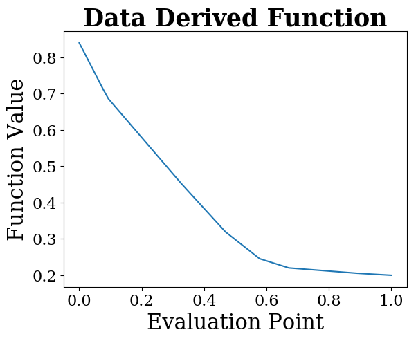
Figure 9: Comparison of active and passive performance on the function depicted in Figure 6. The xx-axis is the number of samples taken, and the yy-axis is L∞L_{\infty} error. Dotted lines denote a least-squares trendline. Refer to caption
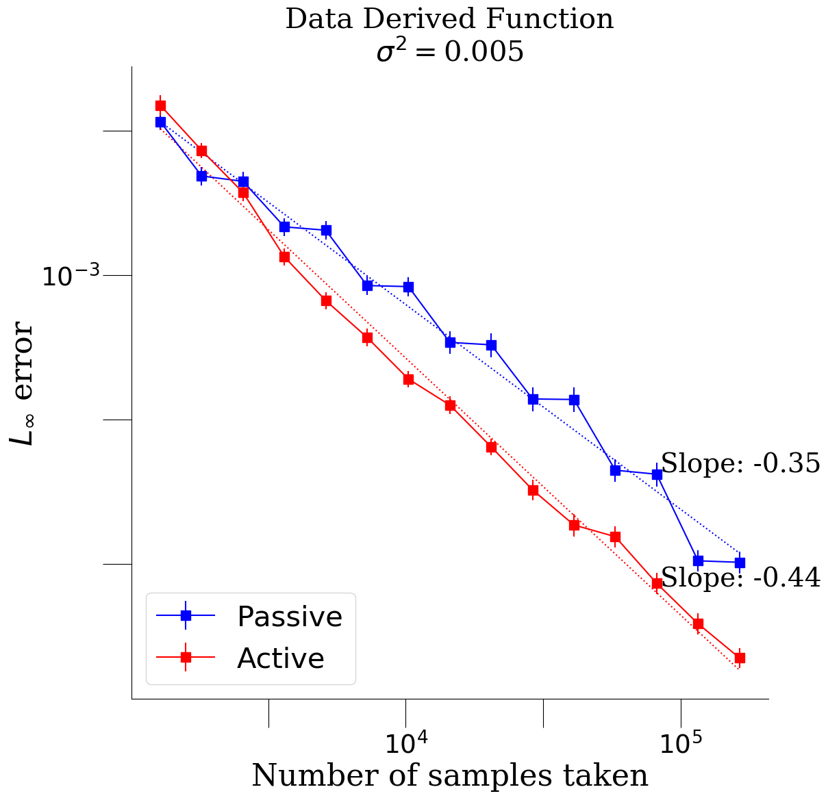
In Figure 9, we compare the performance of the active and passive algorithms for the function ff depicted in Figure 6. Again, the dotted trend lines correspond to a least-squares fit to the logarithmic of the xx and yy coordinates. We find that the passive algorithm appears to obtain a rate of n−1/3n^{-1/3}, and the error of the active algorithm has a scaling closer to that of the parametric rate.

For insight into why the active algorithm fares better on this ff, we can examine the oracle allocations, as constructed in Proposition 3.4. We find that at higher levels of granularity, ff is well approximated by a piecewise linear function, and thus an oracle would only sample at a few, key design points (Figure 12):

Figure 12: A plot of the design points correspond to the oracle allocation constructed in Proposition 3.4, for granularities ϵ∈{.01,.001}\epsilon\in\{.01,.001\}. Bar height is equal to 10001000 divided by the number of design points. Refer to caption

Notice that as the granularity decreases, the oracle allocation refines its design points, dividing the function into regions in which the piecewise-linear approximation holds to a higher accuracy.

7.3 Implementation

The passive algorithm samples at design points xtx_{t} along a dyadic sequence s→=(0,1,1/2,1/4,3/4,1/8,…)\vec{s}=(0,1,1/2,1/4,3/4,1/8,\dots). The algorithm then estimates f⋆f_{\star} using the following constrained least squares problem.

f^∈arg⁡min⁡∑t=1Tf∈ℱconv⁡‖F⁡(xt)−f^‖22.\displaystyle\widehat{f}\in\arg\min_{f\in\mathcal{F}_{\mathrm{conv}}}\sum_{t=1}^{T}\|F(x_{t})-\widehat{f}\|_{2}^{2}~. (23)

We found in practice that this least squares minimization performs surprising well in practice, drastically outperforming projections in the ∞\infty-norm. We used this observation to modify the implementation of our active algorithm. At each round, the active algorithm alternates between sampling a design points x∈{xℓ⁡(I∗),xm⁡(I∗),xr⁡(I∗)}x\in\{x_{\ell(I^{*})},x_{m(I^{*})},x_{r(I^{*})}\} as in Algorithm 2, and sampling dyadic sequences supported on I∗I^{*} given by xℓ⁡(I∗)+|I∗|​s→x_{\ell(I^{*})}+|I^{*}|\vec{s}. We then return f^\widehat{f} using the constrained least-squares problem in (23). In addition, our implementation makes use of the sharper upper- and lower-confidence bounds described in Remark 4.1.

References

  • Bellec et al. [2018] Pierre C Bellec et al. Sharp oracle inequalities for least squares estimators in shape restricted regression. The Annals of Statistics, 46(2):745–780, 2018.
  • Boucheron et al. [2013] Stéphane Boucheron, Gábor Lugosi, and Pascal Massart. Concentration inequalities: A nonasymptotic theory of independence. Oxford University Press, 2013.
  • Cai et al. [2013] T Tony Cai, Mark G Low, Yin Xia, et al. Adaptive confidence intervals for regression functions under shape constraints. The Annals of Statistics, 41(2):722–750, 2013.
  • Castro et al. [2005] Rui Castro, Rebecca Willett, and Robert Nowak. Faster rates in regression via active learning. Advances in Neural Information Processing Systems, 18, 2005.
  • Chatterjee [2016] Sabyasachi Chatterjee. An improved global risk bound in concave regression. Electronic Journal of Statistics, 10(1):1608–1629, 2016.
  • Dümbgen et al. [2004] Lutz Dümbgen, Sandra Freitag, and Geurt Jongbloed. Consistency of concave regression with an application to current-status data. Mathematical Methods of Statistics, 13:69–81, 2004.
  • Dümbgen et al. [2003] Lutz Dümbgen et al. Optimal confidence bands for shape-restricted curves. Bernoulli, 9(3):423–449, 2003.
  • Fisher [1937] Ronald Aylmer Fisher. The design of experiments. Oliver And Boyd; Edinburgh; London, 1937.
  • Frederick et al. [2002] Shane Frederick, George Loewenstein, and Ted O’donoghue. Time discounting and time preference: A critical review. Journal of economic literature, 40(2):351–401, 2002.
  • Green and Myerson [2004] Leonard Green and Joel Myerson. A discounting framework for choice with delayed and probabilistic rewards. Psychological Bulletin, 130(5):769–792, 2004.
  • Guntuboyina and Sen [2015] Adityanand Guntuboyina and Bodhisattva Sen. Global risk bounds and adaptation in univariate convex regression. Probability Theory and Related Fields, 163(1-2):379–411, 2015.
  • Kaufmann et al. [2016] Emilie Kaufmann, Olivier Cappé, and Aurélien Garivier. On the complexity of best-arm identification in multi-armed bandit models. The Journal of Machine Learning Research, 17(1):1–42, 2016.
  • Korostelev [1999] Alexander Korostelev. On minimax rates of convergence in image models under sequential design. Statistics & Probability Letters, 43(4):369–375, 1999.
  • Zhu et al. [2016] Yuancheng Zhu, Sabyasachi Chatterjee, John Duchi, and John Lafferty. Local minimax complexity of stochastic convex optimization. Advances in Neural Information Processing Systems, 29, 2016.

Appendix A Additional Remarks

Remark A.1 (Gap Between Upper and Lower Bounds)

Let ff be a kk-piecewise linear function ff. Then there exists a set of kk intervals ℐ={Ii}1≤i≤k\mathcal{I}=\{I_{i}\}_{1\leq i\leq k} such that ff is linear on each interval; measuring ff at {xl⁡(I),xr⁡(I),xm⁡(I)}I∈ℐ\{x_{l(I)},x_{r(I)},x_{m(I)}\}_{I\in\mathcal{I}} would be enough to estimate ff with zero error over [0,1][0,1]. Hence, we must have N¯​(f,ϵ)≲k\underline{N}(f,\epsilon)\lesssim k. On the other hand, Λavg​(f,ϵ)≈k​log⁡(1/ϵ)\Lambda_{\mathrm{avg}}(f,\epsilon)\approx k\log(1/\epsilon), and indeed one can show that for a kk-piecewise linear function, log⁡(ωmax/ωmin)≈log⁡(1/ϵ)\log(\omega_{\max}/\omega_{\min})\approx\log(1/\epsilon), yielding the necessary cancelation. As with the term log⁡tleft​(f,ϵ)​tright​(f,ϵ)tleft​(f,c​ϵ)​tright​(f,c​ϵ)\log\frac{t_{\mathrm{left}}(f,\epsilon)t_{\mathrm{right}}(f,\epsilon)}{t_{\mathrm{left}}(f,c\epsilon)t_{\mathrm{right}}(f,c\epsilon)}, log⁡(ωmax/ωmin)\log(\omega_{\max}/\omega_{\min}) scales at most as log⁡(1/ϵ)\log(1/\epsilon) for most reasonable functions, and can be bounded by log⁡(maxx∈[0,1]⁡f′′​(x)/minx∈[0,1]⁡f′′​(x))\log(\max_{x\in[0,1]}f^{\prime\prime}(x)/\min_{x\in[0,1]}f^{\prime\prime}(x)) for any twice-differentiable function ff. Overall, we conjecture that the true sample complexity lies closer to N¯​(f,ϵ)\underline{N}(f,\epsilon), because in the noiseless setting, one can approximate left- and right-derivatives of ff to arbitrary accuracy using just two points. This makes it possible to learn a 2-piecewise linear function with a constant number of function evaluations, rather than the O⁡(log⁡(1/ϵ))O(\log(1/\epsilon)) implied by Λ⁡(f,ϵ)\Lambda(f,\epsilon).

Remark A.2 (Sub-Optimality of Non-Uniform Designs)

In this remark, we argue that although non-uniform designs can improve upon uniform designs for some functions of interest, in general they provide no benefit.

To present the argument, we begin with by recalling the proof of Theorem 3.6. We argued that given f∈ℱconvf\in\mathcal{F}_{\mathrm{conv}} and x0∈[tleft(f,2ϵ),1−tright(f,2ϵ))]x_{0}\in[t_{\mathrm{left}}(f,2\epsilon),1-t_{\mathrm{right}}(f,2\epsilon))], then unless a design collects ≳(1+σ2ϵ2)​log⁡(1/δ)\gtrsim(1+\frac{\sigma^{2}}{\epsilon^{2}})\log(1/\delta) samples in the interior of the interval I0:=[x0−ω⁡(f,x0,2​ϵ),x0+ω⁡(f,x0,2​ϵ)]I_{0}:=[x_{0}-\omega(f,x_{0},2\epsilon),x_{0}+\omega(f,x_{0},2\epsilon)], the alternative function

f~​(x):=f⁡(x)+𝕀⁡(x∈I0)⋅(Sec⁡[f,I0]​(x)−f⁡(x))\displaystyle\widetilde{f}(x):=f(x)+\mathbb{I}(x\in I_{0})\cdot\left(\mathrm{Sec}[f,I_{0}](x)-f(x)\right)

satisfies supg∈{f,f~}ℙ𝖠𝗅𝗀,g[∥f^−g∥∞≥ϵ]≥δ\sup_{g\in\{f,\widetilde{f}\}}\mathbb{P}_{\mathsf{Alg},g}[\|\widehat{f}-g\|_{\infty}\geq\epsilon]\geq\delta. In Theorem 3.6, we chose x0=x∗:=argmin{ω(f,x,2ϵ)|x∈[tleft(f,2ϵ),1−tright(f,2ϵ))]}x_{0}=x_{*}:=\arg\min\{\omega(f,x,2\epsilon)|x\in[t_{\mathrm{left}}(f,2\epsilon),1-t_{\mathrm{right}}(f,2\epsilon))]\}, and defined I∗I_{*} analogously. By uniformity, the design could not oversample in the interior of I∗I_{*}, and thus the total number of samples collected, up to constants, would need to be

1|I∗|​(1+σ2ϵ2)​log⁡(1/δ)≳Λmax​(f,2​ϵ)⋅(1+σ2ϵ2)​log⁡(1/δ).\displaystyle\frac{1}{|I_{*}|}(1+\frac{\sigma^{2}}{\epsilon^{2}})\log(1/\delta)\gtrsim\Lambda_{\mathrm{max}}(f,2\epsilon)\cdot(1+\frac{\sigma^{2}}{\epsilon^{2}})\log(1/\delta)~.

Without uniformity, we cannot rule out that the design concentrates its samples in I∗I_{*}. Nevertheless, we can show that there is a function “similar” to ff which incurs the same lower bound. For ease, assume that ff is right differentiable at x=1x=1 and left differentiable at x=0x=0.11 1 In general, ff is convex and thus right differentiable at 1−η1-\eta and left differentiable at η\eta for all η>0\eta>0. Hence, one can modify ff with a linear extension to [0,η][0,\eta] and [1−η,1][1-\eta,1] to ensure that this condition holds. Letting ∂−\partial_{-} and ∂+\partial_{+} denote the right- and left-derivative, we can define the shift function as

f←t​(x):={f⁡(x−t)x∈[0∨t,1∧1+t]f⁡(1)+(x−1−t)​∂−f⁡(1)x≥1−t,t<0,f⁡(0)+(t−x)​∂+f⁡(0)x≤t,t>0.\displaystyle f_{\leftarrow t}(x):=\begin{cases}f(x-t)&x\in[0\vee t,1\wedge 1+t]\\ f(1)+(x-1-t)\partial_{-}f(1)&x\geq 1-t,t<0,\\ f(0)+(t-x)\partial_{+}f(0)&x\leq t,t>0\end{cases}.

We observe that f←tf_{\leftarrow t} is convex, and if x∗x^{*} is as above, then for any t∈(x∗+ω⁡(f,x∗,2​ϵ)−1,x∗−ω⁡(f,x∗,2​ϵ))t\in(x^{*}+\omega(f,x^{*},2\epsilon)-1,x^{*}-\omega(f,x^{*},2\epsilon)), one can verify that

ω⁡(f←t,x∗+t,2​ϵ)=ω⁡(f,x∗,2​ϵ).\displaystyle\omega(f_{\leftarrow t},x^{*}+t,2\epsilon)=\omega(f,x^{*},2\epsilon)~.

Then, for any interval Ibad=[a,b]⊂[0,1]I_{\mathrm{bad}}=[a,b]\subset[0,1] for which |Ibad|≥2​Iℓ∗|I_{\mathrm{bad}}|\geq 2I^{*}_{\ell}, there exists a tbad∈ℝt_{\mathrm{bad}}\in\mathbb{R} such that I←tbad∗:=I∗+tbad​|I∗|⊂IbadI^{*}_{\leftarrow t_{\mathrm{bad}}}:=I^{*}+t_{\mathrm{bad}}|I^{*}|\subset I_{\mathrm{bad}}. Hence, if 𝔼[|xt:xt∈Ibad|]≪σ2log(1/δ)\mathbb{E}[|x_{t}:x_{t}\in I_{\mathrm{bad}}|]\ll\sigma^{2}\log(1/\delta), then even if the passive design can estimate ff correctly, it will fail to distinguish between the shifted function f←tbadf_{\leftarrow t_{\mathrm{bad}}} and the shifted alternative:

f~←tbad​(x):=f←tbad​(x)+𝕀⁡(x∈I←tbad∗)​(Sec⁡[f←tbad,I←tbad∗]​(x)−f←tbad​(x)).\displaystyle\widetilde{f}_{\leftarrow t_{\mathrm{bad}}}(x):=f_{\leftarrow t_{\mathrm{bad}}}(x)+\mathbb{I}(x\in I^{*}_{\leftarrow t_{\mathrm{bad}}})(\mathrm{Sec}[f_{\leftarrow t_{\mathrm{bad}}},I^{*}_{\leftarrow t_{\mathrm{bad}}}](x)-f_{\leftarrow t_{\mathrm{bad}}}(x)).

As a consequence, any algorithm which is δ\delta-correct for all ff shifts f←tf_{\leftarrow t}, and alternatives defined above must collect at least ≳σ2​log⁡(1/δ)⋅ω​(f,x∗,2​ϵ)−1\gtrsim\sigma^{2}\log(1/\delta)\cdot\omega(f,x^{*},2\epsilon)^{-1} samples. The above argument can also be extended to the case where the shift tbadt_{\mathrm{bad}} is chosen at random (as opposed to depending on the design).