跳到论文正文
W Papers独立论文阅读器 arXiv:1808.04236 论文正文 计算阅读时间 · 0%
引用这篇论文根据当前论文元数据生成,正式投稿前建议核对。


License: arXiv.org perpetual non-exclusive license
arXiv:1808.04236v1 [hep-ph] 13 Aug 2018

Lowest-order electron-electron and electron-muon scattering in a strong magnetic field

Abhishek Tiwari†11 1 abhi7phy@gmail.com and Binoy Krishna Patra† 22 2 binoyfph@iitr.ac.in

† Department of Physics, Indian Institute of Technology Roorkee, Roorkee 247 667, India

Abstract

In this work we have investigated how the much studied scattering processes in vacuum at the lowest-order, viz. electron-muon (ee-μ\mu) scattering in both ss- and tt-channel, Bhabha scattering, and Møller scattering, have been modified in the presence of a strong magnetic field (|e​B|>>m2|eB|>>m^{2}, mm is the mass of electron or muon). For that purpose, we have first calculated the square of the matrix element by summing over the spin states, using the spinors in the presence of a strong magnetic field and then obtain the crosssection by integrating over the available phase space for the final states and averaging over the initial states. The first noticeable observation in the spin-summed of the matrix element squared is that the interference term between ss- and tt-channel and tt- and uu-channel in Bhabha and Møller scattering, respectively are missing in the presence of strong magnetic field. We have found that in the presence of strong magnetic field, the crosssection of e−​e+→μ−​μ+e^{-}e^{+}\rightarrow\mu^{-}\mu^{+} annihilation process in the lowest order decreases inversely proportional to the fourth power of the center-of-mass energy (s\sqrt{s}), compared to the inversely proportional to the square of center-of-mass energy in vacuum alone. Like in vacuum, the crosssection for ee-μ\mu scattering in t{\rm t} channel, i.e. for e−​μ−→e−​μ−e^{-}\mu^{-}\rightarrow e^{-}\mu^{-} process, even in a strong magnetic field too diverges but the finite part decreases with s\sqrt{s} much faster than in vacuum alone. Similarly the crosssections for both Bhabha and Møller scattering at the lowest-order diverges in the infrared limit. However, the finite term decreases with s\sqrt{s} much faster than the vacuum alone. In addition there is finite negative contribution, which is independent of s\sqrt{s} and decreases with the magnetic field.

PACS: 12.39.-x,11.10.St,12.38.Mh,12.39.Pn 12.75.N, 12.38.G

Keywords: Dirac spinor, electron-electron scattering, electron-muon scattering, strong magnetic field, crosssection, Mandelstam and magnetic Mandelstam variables

1 Introduction

The relativistic heavy-ion collider (RHIC) at the Brookhaven National Laboratory, USA, with the center-of-mass energy, s\sqrt{s}= 200 GeV per nucleon in Au - Au collisions and the large hadron collider (LHC) at the European Organization for Nuclear Research, Geneva, with s\sqrt{s} = 2.76 TeV per nucleon in Pb-Pb collisions may have produced intensely strong magnetic field at very early stages of collisions, when the event is off-central [1, 2, 3, 4, 5]. Depending on the centralities, the strength of the magnetic field may reach between mπ2m_{\pi}^{2} (≃1018\simeq 10^{18} Gauss) at RHIC [6] to 15 mπ2m_{\pi}^{2} at LHC [7]. At extreme cases it may reach values of 50 mπ2m_{\pi}^{2} at LHC. A very strong magnetic field (∼1023\sim 10^{23} Gauss) may have existed in the early universe during the electroweak phase transition due to the gradients in Higgs field [8] or at the core of magnetars [9].

Thus we are motivated in this work to study the different processes in electron-muon and electron-electron scattering in the lowest order in the presence of strong magnetic field. However, the above processes in the lowest as well as higher order are well studied theoretically in vacuum [10, 11, 12] with the solutions of Dirac equation in vacuum, i.e. with the free Dirac spinors for positive and negative energy and their corresponding completeness relation. However, the scenario in the presence of strong magnetic field is different because the form of the Dirac spinors are going to change, where, apart from the momentum dependence, the spinors also depend on the spatial coordinates due to the gauge used to solve the Dirac equation in magnetic field. As a result, the completeness relations are also going to change. For the sake of simplicity we assume the magnetic field to be uniform and stationary. Moreover the strength of the magnetic field is strong enough so that only the lowest Landau level is sufficient for the calculation of the matrix element and the crosssection.

This paper is divided into following sections. We first nomenclature the four-momentum, Mandelstam variables, magnetic Mandelstam variables, suitable for the description in a strong magnetic field and then revisit the Dirac equation in a strong and homogeneous magnetic field in section 2.1 and 2.2, respectively. Using those notations, we calculate the spin-summed matrix element squared for the electron-muon scattering ss-channel (annihilation process) and tt- channel, Bhabha scattering and Møller scattering in sections 2.3-2.5, respectively. In section 3, we first revisit for the formula for calculating the crosssection by constructing the Lorentz invariant phase space, flux factor, energy-momentum conserving Dirac-Delta function etc. in the presence of strong magnetic field and then using the the matrix elements for the above processes from the above sections 2.3-2.5, the corresponding crosssections have been evaluated in sections 3.1-3.4, respectively. Finally we conclude our results and discussion in section 4.

2 Electron-Electron and Electron-Muon Scattering in Strong Magnetic field

Our aim in this section is to calculate the square of matrix element for the electron-muon scattering in both ss- and tt-channel, Bhabha scattering, and Møller scattering in a strong homogeneous magnetic field. For the sake of simplicity we work in the extreme relativistic limit, where we neglect the masses of electrons as well as muons. In the presence of magnetic field the form of spinor and hence the form of electron propagator is changed but the form of photon propagator remains the same. So first we are going to revisit the Dirac equation in the strong magnetic field to obtain the form of positive energy and negative energy spinors and their completeness relations.

2.1 Notations

Refer to caption
Figure 1:

The dynamics of an electron in a magnetic field is factorized into transverse and longitudinal plane with respect to the direction of magnetic field, as a result its momentum (𝐩\mathbf{p}) is separated into perpendicular and longitudinal components with respect to the direction of magnetic field (say, zz-direction). Hence the dispersion relation is modified quantum mechanically into

En​(pz)=pz2+mf2+2​n​|e​B|,\displaystyle E_{n}(p_{z})=\sqrt{p_{z}^{2}+m_{f}^{2}+2n\left|eB\right|}\quad, (1)

In a strong magnetic field (|e​B|>>m2|eB|>>m^{2}), electrons prefer to lie in the lowest Landau level, hence the electron momentum becomes purely longitudinal [13], i.e 𝒑⟂≈0\mathchoice{\mbox{\boldmath$p$}}{\mbox{\boldmath$p$}}{\mbox{\boldmath$\scriptstyle p$}}{\mbox{\boldmath$\scriptscriptstyle p$}}_{\perp}\approx 0. The aforesaid observation motivates to construct the following kinematic variables, viz. momentum, Mandelstam variables etc. which will be advantageous to express matrix element squared, crosssection etc. in a strong magnetic field. Thus using the following convention of the metric tensor

gμ​ν=(1,−1,−1,−1),gμ⟂​ν⟂=(0,−1,−1,0)​and​gμ∥​ν∥=(1,0,0,−1),\displaystyle g^{\mu\nu}=(1,-1,-1,-1),g^{\mu_{\perp}\nu_{\perp}}=(0,-1,-1,0)\penalty\ {\rm and}\penalty\ g^{\mu_{\parallel}\nu_{\parallel}}=(1,0,0,-1)\penalty\ , (2)

we will first denote the four-momentum for a generic Feynman diagram in Figure 1,

p⟂μ\displaystyle p_{\perp}^{\mu} =\displaystyle= (0,p1,p2,0)=(0,px,py,0),\displaystyle(0,p^{1},p^{2},0)=(0,p_{x},p_{y},0), (3)
p∥μ\displaystyle p_{\parallel}^{\mu} =\displaystyle= (p0,0,0,p3)=(E0,0,0,pz),\displaystyle(p^{0},0,0,p^{3})=(E_{0},0,0,p_{z}), (4)
p∥~μ\displaystyle\widetilde{p_{\parallel}}^{\mu} =\displaystyle= (p~0,0,0,p~3)=(p3,0,0,p0),\displaystyle(\widetilde{p}^{0},0,0,\widetilde{p}^{3})=(p^{3},0,0,p^{0}), (5)

therefore the usual Mandelstam variables take the following form:

s\displaystyle s =\displaystyle= (p∥+k∥)2=(P∥+K∥)2,\displaystyle(p_{\parallel}+k_{\parallel})^{2}=(P_{\parallel}+K_{\parallel})^{2}, (6)
t\displaystyle t =\displaystyle= (p∥−P∥)2=(K∥−k∥)2,\displaystyle(p_{\parallel}-P_{\parallel})^{2}=(K_{\parallel}-k_{\parallel})^{2}, (7)
u\displaystyle u =\displaystyle= (p∥−K∥)2=(P∥−k∥)2.\displaystyle(p_{\parallel}-K_{\parallel})^{2}=(P_{\parallel}-k_{\parallel})^{2}. (8)

We define some new variables sp,sk,sP,sK,tp,tP,tK,tk,up,uk,uP,uKs_{p},s_{k},s_{P},s_{K},t_{p},t_{P},t_{K},t_{k},u_{p},u_{k},u_{P},u_{K}, dubbed as the magnetic Mandelstam variables, which are defined as

sp\displaystyle s_{p} =\displaystyle= (p~∥+k∥)2,sk=(k~∥+p∥)2,\displaystyle(\widetilde{p}_{\parallel}+k_{\parallel})^{2},\penalty\ s_{k}=(\widetilde{k}_{\parallel}+p_{\parallel})^{2}, (9)
sP\displaystyle s_{P} =\displaystyle= (P~∥+K∥)2,sK=(K~∥+P∥)2,\displaystyle(\widetilde{P}_{\parallel}+K_{\parallel})^{2},\penalty\ s_{K}=(\widetilde{K}_{\parallel}+P_{\parallel})^{2}, (10)
tp\displaystyle t_{p} =\displaystyle= (p~∥−P∥)2,tP=(P~∥−p∥)2,\displaystyle(\widetilde{p}_{\parallel}-P_{\parallel})^{2},\penalty\ t_{P}=(\widetilde{P}_{\parallel}-p_{\parallel})^{2}, (11)
tK\displaystyle t_{K} =\displaystyle= (K~∥−k∥)2,tk=(k~∥−K∥)2,\displaystyle(\widetilde{K}_{\parallel}-k_{\parallel})^{2},\penalty\ t_{k}=(\widetilde{k}_{\parallel}-K_{\parallel})^{2}, (12)
up\displaystyle u_{p} =\displaystyle= (p~∥−K∥)2,uK=(K~∥−p∥)2,\displaystyle(\widetilde{p}_{\parallel}-K_{\parallel})^{2},\penalty\ u_{K}=(\widetilde{K}_{\parallel}-p_{\parallel})^{2}, (13)
uP\displaystyle u_{P} =\displaystyle= (P~∥−k∥)2,uk=(k~∥−P∥)2.\displaystyle(\widetilde{P}_{\parallel}-k_{\parallel})^{2},\penalty\ u_{k}=(\widetilde{k}_{\parallel}-P_{\parallel})^{2}. (14)

Although the form of the magnetic Mandelstam variables (or the half-tilde Mandelstam variables, where one momentum is tilde) are same as the Mandelstam variables but they are completely different from them. In the extreme relativistic limit, they satisfy the following relations among themselves

sp=−sk,\displaystyle s_{p}=-s_{k}, sP=−sK,\displaystyle s_{P}=-s_{K}, (15)
tp=−tP,\displaystyle t_{p}=-t_{P}, tK=−tk,\displaystyle t_{K}=-t_{k}, (16)
up=−uK,\displaystyle u_{p}=-u_{K}, uP=−uk.\displaystyle u_{P}=-u_{k}. (17)

Furthermore we use other notations for the full-tilde Mandelstam variables, which are defined as

s~\displaystyle\widetilde{s} =\displaystyle= (p~∥+k~∥)2=(P~∥+K~∥)2,\displaystyle(\widetilde{p}_{\parallel}+\widetilde{k}_{\parallel})^{2}=(\widetilde{P}_{\parallel}+\widetilde{K}_{\parallel})^{2}, (18)
t~\displaystyle\widetilde{t} =\displaystyle= (p~∥−P~∥)2=(K~∥−k~∥)2,\displaystyle(\widetilde{p}_{\parallel}-\widetilde{P}_{\parallel})^{2}=(\widetilde{K}_{\parallel}-\widetilde{k}_{\parallel})^{2}, (19)
u~\displaystyle\widetilde{u} =\displaystyle= (p~∥−K~∥)2=(P~∥−k~∥)2.\displaystyle(\widetilde{p}_{\parallel}-\widetilde{K}_{\parallel})^{2}=(\widetilde{P}_{\parallel}-\widetilde{k}_{\parallel})^{2}. (20)

We can directly relate the full-tilde Mandelstam variables to the Mandelstam variables as

s=−s~,t=−t~,u=−u~.\displaystyle s=-\widetilde{s},\penalty\ t=-\widetilde{t},\penalty\ u=-\widetilde{u}\penalty\ . (21)

2.2 Dirac Spinors in a strong magnetic field

The methods of Ritus eigenfunction [14] along with the Schwinger Proper-time formalism [15] are commonly used to solved the Dirac equation of charged fermions in the presence of a constant magnetic field. There are different ways which have been adopted in the literature [16, 17, 18] to obtain the spinor in a magnetic field, however, we have mainly adopted to solve the Dirac equation in a constant external field from Ref. [19].

For the sake of simplicity, we assume a static and homogeneous magnetic field, which is along the zz-direction, 𝑩=B​z^\mathchoice{\mbox{\boldmath$B$}}{\mbox{\boldmath$B$}}{\mbox{\boldmath$\scriptstyle B$}}{\mbox{\boldmath$\scriptscriptstyle B$}}=B\hat{z}. Such a magnetic field can be obtained from a vector potential Aμ=(0,0,B​x,0)A^{\mu}=(0,0,Bx,0). The choice of vector potential is not unique as the same magnetic field can also be obtained from a symmetric potential given by Aμ=(0,−B​y2,B​x2,0)A^{\mu}=(0,\frac{-By}{2},\frac{Bx}{2},0). Thus the positive energy Dirac spinors with the gauge Aμ=(0,−B​y,0,0)A^{\mu}=(0,-By,0,0) are given by the shifted coordinate, ξ\xi (=e​B​(y−pxe​B)\sqrt{eB}\left(y-\frac{p_{x}}{eB}\right)) [20, 19]

U+(y,n,𝒑\y)=N(In−1​(ξ)0pzEn+m​In−1​(ξ)−2​n​e​BEn+m​In​(ξ));U−(y,n,𝒑\y)=N(0In​(ξ)−2​n​e​BEn+m​In−1​(ξ)−pzEn+m​In​(ξ))\displaystyle U_{+}(y,n,\mathchoice{\mbox{\boldmath$p$}}{\mbox{\boldmath$p$}}{\mbox{\boldmath$\scriptstyle p$}}{\mbox{\boldmath$\scriptscriptstyle p$}}_{{}_{\!\hbox to0.0pt{$\scriptscriptstyle\backslash$\hss}{\scriptscriptstyle y}}})=N\left(\begin{array}[]{c}I_{n-1}(\xi)\\[8.61108pt] 0\\[8.61108pt] {\textstyle p_{z}\over\textstyle E_{n}+m}I_{n-1}(\xi)\\[8.61108pt] -\,{\textstyle\sqrt{2neB}\over\textstyle E_{n}+m}I_{n}(\xi)\end{array}\right);\hskip 5.69054ptU_{-}(y,n,\mathchoice{\mbox{\boldmath$p$}}{\mbox{\boldmath$p$}}{\mbox{\boldmath$\scriptstyle p$}}{\mbox{\boldmath$\scriptscriptstyle p$}}_{{}_{\!\hbox to0.0pt{$\scriptscriptstyle\backslash$\hss}{\scriptscriptstyle y}}})=N\left(\begin{array}[]{c}0\\[8.61108pt] I_{n}(\xi)\\[8.61108pt] -\,{\textstyle\sqrt{2neB}\over\textstyle E_{n}+m}I_{n-1}(\xi)\\[8.61108pt] -\,{\textstyle p_{z}\over\textstyle E_{n}+m}I_{n}(\xi)\end{array}\right)

Similarly the negative energy Dirac spinors with ξ~\widetilde{\xi} (=e​B​(y+pxe​B)\sqrt{eB}\left(y+\frac{p_{x}}{eB}\right)) are given by [20, 19]

V−(y,n,𝒑\y)=N(pzEn+m​In−1​(ξ~)2​n​e​BEn+m​In​(ξ~)In−1​(ξ~)0);V+(y,n,𝒑\y)=N(2​n​e​BEn+m​In−1​(ξ~)−pzEn+m​In​(ξ~)0In​(ξ~))\displaystyle V_{-}(y,n,\mathchoice{\mbox{\boldmath$p$}}{\mbox{\boldmath$p$}}{\mbox{\boldmath$\scriptstyle p$}}{\mbox{\boldmath$\scriptscriptstyle p$}}_{{}_{\!\hbox to0.0pt{$\scriptscriptstyle\backslash$\hss}{\scriptscriptstyle y}}})=N\left(\begin{array}[]{c}{\textstyle p_{z}\over\textstyle E_{n}+m}I_{n-1}(\widetilde{\xi})\\[8.61108pt] {\textstyle\sqrt{2neB}\over\textstyle E_{n}+m}I_{n}(\widetilde{\xi})\\[8.61108pt] I_{n-1}(\widetilde{\xi})\\[8.61108pt] 0\end{array}\right);\hskip 5.69054ptV_{+}(y,n,\mathchoice{\mbox{\boldmath$p$}}{\mbox{\boldmath$p$}}{\mbox{\boldmath$\scriptstyle p$}}{\mbox{\boldmath$\scriptscriptstyle p$}}_{{}_{\!\hbox to0.0pt{$\scriptscriptstyle\backslash$\hss}{\scriptscriptstyle y}}})=N\left(\begin{array}[]{c}{\textstyle\sqrt{2neB}\over\textstyle E_{n}+m}I_{n-1}(\widetilde{\xi})\\[8.61108pt] -\,{\textstyle p_{z}\over\textstyle E_{n}+m}I_{n}(\widetilde{\xi})\\[8.61108pt] 0\\[8.61108pt] I_{n}(\widetilde{\xi})\end{array}\right)\,

where the normalization constant (NN) is N=En+mN=\sqrt{E_{n}+m} and the symbol, p\yp_{{}_{\!\hbox to0.0pt{$\scriptscriptstyle\backslash$\hss}{\scriptscriptstyle y}}} denotes the absence of the yy-component of momentum in the spinors. The energy eigenvalues are given by the above Landau quantization (1), where nn denotes the Landau levels and the energy eigenfunctions, In​(ξ)I_{n}(\xi) are expressed in terms of Hermite polynomials, Hn​(ξ)H_{n}(\xi)

In​(ξ)\displaystyle I_{n}(\xi) =\displaystyle= e​Bn!​2n​π​e−ξ22​Hn​(ξ),\displaystyle\frac{\sqrt{eB}}{n!2^{n}\sqrt{\pi}}e^{\frac{-\xi^{2}}{2}}H_{n}(\xi), (40)

with the properties: I−1​(ξ)=0I_{-1}(\xi)=0 and I02​(ξ)=1I_{0}^{2}(\xi)=1. As mentioned earlier, in a strong magnetic field, only the lowest Landau level (n=0) is populated.

We can now calculate the spin sums for the particles (PUP_{U}) and anti-particles (PVP_{V}) in the presence of external magnetic field as [20, 19]

PU​(y,y′,n,𝒑\y)\displaystyle P_{U}(y,y^{\prime},n,\mathchoice{\mbox{\boldmath$p$}}{\mbox{\boldmath$p$}}{\mbox{\boldmath$\scriptstyle p$}}{\mbox{\boldmath$\scriptscriptstyle p$}}_{\!\hbox to0.0pt{$\scriptscriptstyle\backslash$\hss}{\scriptscriptstyle y}}) =\displaystyle= ∑sUs(y,n,𝒑\y)U¯s(y′,n,𝒑\y)\displaystyle\sum_{\rm s}U_{s}(y,n,\mathchoice{\mbox{\boldmath$p$}}{\mbox{\boldmath$p$}}{\mbox{\boldmath$\scriptstyle p$}}{\mbox{\boldmath$\scriptscriptstyle p$}}_{{}_{\!\hbox to0.0pt{$\scriptscriptstyle\backslash$\hss}{\scriptscriptstyle y}}})\overline{U}_{s}(y^{\prime},n,\mathchoice{\mbox{\boldmath$p$}}{\mbox{\boldmath$p$}}{\mbox{\boldmath$\scriptstyle p$}}{\mbox{\boldmath$\scriptscriptstyle p$}}_{{}_{\!\hbox to0.0pt{$\scriptscriptstyle\backslash$\hss}{\scriptscriptstyle y}}}) (41)
=\displaystyle= 12[{m(1+Σz)+/p∥−/​p~∥γ5}In−1(ξ)In−1(ξ′)\displaystyle{1\over 2}\bigg[\left\{m(1+\Sigma_{z})+\hbox to0.0pt{/\hss}p_{\parallel}-\widetilde{\hbox to0.0pt{/\hss}p}_{\parallel}\gamma_{5}\right\}I_{n-1}(\xi)I_{n-1}(\xi^{\prime})
+\displaystyle+ {m⁡(1−Σz)+/​p∥−γ5​/​p~∥}​In​(ξ)​In​(ξ′)\displaystyle\left\{m(1-\Sigma_{z})+\hbox to0.0pt{/\hss}p_{\parallel}-\gamma_{5}\widetilde{\hbox to0.0pt{/\hss}p}_{\parallel}\right\}I_{n}(\xi)I_{n}(\xi^{\prime})
−\displaystyle- 2​n​e​B​(γ1−i​γ2)​In​(ξ)​In−1​(ξ′)\displaystyle\sqrt{2neB}(\gamma_{1}-i\gamma_{2})I_{n}(\xi)I_{n-1}(\xi^{\prime})
−\displaystyle- 2​n​e​B(γ1+iγ2)In−1(ξ)In(ξ′)],\displaystyle\sqrt{2neB}(\gamma_{1}+i\gamma_{2})I_{n-1}(\xi)I_{n}(\xi^{\prime})\bigg],
PV​(y~,y′~,n,𝒑\y)\displaystyle P_{V}(\widetilde{y},\widetilde{y^{\prime}},n,\mathchoice{\mbox{\boldmath$p$}}{\mbox{\boldmath$p$}}{\mbox{\boldmath$\scriptstyle p$}}{\mbox{\boldmath$\scriptscriptstyle p$}}_{\!\hbox to0.0pt{$\scriptscriptstyle\backslash$\hss}{\scriptscriptstyle y}}) =\displaystyle= ∑sVs(y~,n,𝒑\y)V¯s(y′~,n,𝒑\y)\displaystyle\sum_{\rm s}V_{s}(\widetilde{y},n,\mathchoice{\mbox{\boldmath$p$}}{\mbox{\boldmath$p$}}{\mbox{\boldmath$\scriptstyle p$}}{\mbox{\boldmath$\scriptscriptstyle p$}}_{{}_{\!\hbox to0.0pt{$\scriptscriptstyle\backslash$\hss}{\scriptscriptstyle y}}})\overline{V}_{s}(\widetilde{y^{\prime}},n,\mathchoice{\mbox{\boldmath$p$}}{\mbox{\boldmath$p$}}{\mbox{\boldmath$\scriptstyle p$}}{\mbox{\boldmath$\scriptscriptstyle p$}}_{{}_{\!\hbox to0.0pt{$\scriptscriptstyle\backslash$\hss}{\scriptscriptstyle y}}}) (42)
=\displaystyle= 12[{−m(1+Σz)+/p∥−/​p~∥γ5}In−1(ξ~)In−1(ξ~′)\displaystyle{1\over 2}\Bigg[\left\{-m(1+\Sigma_{z})+\hbox to0.0pt{/\hss}p_{\parallel}-\widetilde{\hbox to0.0pt{/\hss}p}_{\parallel}\gamma_{5}\right\}I_{n-1}(\widetilde{\xi})I_{n-1}(\widetilde{\xi}^{\prime})
+\displaystyle+ {−m⁡(1−Σz)+/​p∥−γ5​/​p~∥}​In​(ξ~)​In​(ξ~′)\displaystyle\left\{-m(1-\Sigma_{z})+\hbox to0.0pt{/\hss}p_{\parallel}-\gamma_{5}\widetilde{\hbox to0.0pt{/\hss}p}_{\parallel}\right\}I_{n}(\widetilde{\xi})I_{n}(\widetilde{\xi}^{\prime})
+\displaystyle+ 2​n​e​B​(γ1−i​γ2)​In​(ξ~)​In−1​(ξ~′)\displaystyle\sqrt{2neB}(\gamma_{1}-i\gamma_{2})I_{n}(\widetilde{\xi})I_{n-1}(\widetilde{\xi}^{\prime})
+\displaystyle+ 2​n​e​B(γ1+iγ2)In−1(ξ~)In(ξ~′)],\displaystyle\sqrt{2neB}(\gamma_{1}+i\gamma_{2})I_{n-1}(\widetilde{\xi})I_{n}(\widetilde{\xi}^{\prime})\Bigg],\,

where Σz=i​γ1​γ2\Sigma_{z}=i\gamma^{1}\gamma^{2}, p̸∥=p0​γ0−p3​γ3\not{p}_{\parallel}=p^{0}\gamma^{0}-p^{3}\gamma^{3}, p̸~∥=p3​γ0−p0​γ3\widetilde{\not{p}}_{\parallel}=p^{3}\gamma^{0}-p^{0}\gamma^{3} and mm is the mass of electron.

2.3 Matrix element for electron-muon scattering at the lowest-order

There are two different processes for electron-muon scattering, viz. (e−​e+→μ−​μ+)(e^{-}e^{+}\rightarrow\mu^{-}\mu^{+}) and (e−​μ−→e−​μ−)(e^{-}\mu^{-}\rightarrow e^{-}\mu^{-}) represented by ss and tt-channel diagrams, respectively. We will first evaluate the matrix element (𝔐\mathfrak{M}) for the ss-channel diagram and calculate the |𝔐|2¯\overline{\left|\mathfrak{M}\right|^{2}} by summing over the spin states. Finally we calculate the same for the tt-channel process.

ss-Channel Process:
The electron-muon scattering in ss-channel represents the e−​e+→μ−​μ+e^{-}e^{+}\rightarrow\mu^{-}\mu^{+} process by the following Feynman diagram at the lowest-order in Figure 2.

Refer to caption
Figure 2: ss-channel

where UU and U¯\overline{U} denote the Dirac spinors for the incoming and the outgoing fermions, respectively whereas VV and V¯\overline{V} in Figure 2 represent the spinors for the outgoing and the incoming anti-fermions, respectively. Therefore the invariant amplitude for the e−​e+→μ−​μ+e^{-}e^{+}\rightarrow\mu^{-}\mu^{+} process at the lowest-order is given by the matrix element,

−i​𝔐s​(e−​e+→μ−​μ+)\displaystyle-i\mathfrak{M}_{\rm s}(e^{-}e^{+}\rightarrow\mu^{-}\mu^{+}) =\displaystyle= [V¯(yB,k\y)ieγμU(yA,p\y)](−i​gμ​νq2)[U¯(YC,P\y)ieγνV(YD,K\y)].\displaystyle\big[\overline{V}(y_{B},k_{{}_{\!\hbox to0.0pt{$\scriptscriptstyle\backslash$\hss}{\scriptscriptstyle y}}})ie\gamma^{\mu}U(y_{A},p_{{}_{\!\hbox to0.0pt{$\scriptscriptstyle\backslash$\hss}{\scriptscriptstyle y}}})\big]\left(\frac{-ig^{\mu\nu}}{q^{2}}\right)\big[\overline{U}(Y_{C},P_{{}_{\!\hbox to0.0pt{$\scriptscriptstyle\backslash$\hss}{\scriptscriptstyle y}}})ie\gamma^{\nu}V(Y_{D},K_{{}_{\!\hbox to0.0pt{$\scriptscriptstyle\backslash$\hss}{\scriptscriptstyle y}}})\big]. (43)

We will now calculate the square of the matrix element, |𝔐s|2{\left|\mathfrak{M}_{s}\right|}^{2} and then sum over the spin-states. It is convenient and easy to solve if we separately write the spin sums for electron and muon

|𝔐s|2¯​(e−​e+→μ−​μ+)=e4q4​Leμ​ν​Lμ​νm​u​o​n,\overline{\left|\mathfrak{M}_{\rm s}\right|^{2}}{(e^{-}e^{+}\rightarrow\mu^{-}\mu^{+})}=\frac{e^{4}}{q^{4}}L_{e}^{\mu\nu}L^{muon}_{\mu\nu}, (44)

where the Leμ​νL_{e}^{\mu\nu} and Lμ​νmuonL^{\rm{muon}}_{\mu\nu} are given by

Leμ​ν\displaystyle L_{e}^{\mu\nu} =\displaystyle= ∑e​s​p​i​n​s[V¯(yB,k\y)γμU(yA,p\y)][V¯(yB,k\y)γνU(yA,p\y)]∗,\displaystyle\sum_{e\penalty\ spins}\big[\overline{V}(y_{B},k_{{}_{\!\hbox to0.0pt{$\scriptscriptstyle\backslash$\hss}{\scriptscriptstyle y}}})\gamma^{\mu}U(y_{A},p_{{}_{\!\hbox to0.0pt{$\scriptscriptstyle\backslash$\hss}{\scriptscriptstyle y}}})\big]\big[\overline{V}(y_{B},k_{{}_{\!\hbox to0.0pt{$\scriptscriptstyle\backslash$\hss}{\scriptscriptstyle y}}})\gamma^{\nu}U(y_{A},p_{{}_{\!\hbox to0.0pt{$\scriptscriptstyle\backslash$\hss}{\scriptscriptstyle y}}})\big]^{*}\penalty\ , (45)
Lμ​νm​u​o​n\displaystyle L^{muon}_{\mu\nu} =\displaystyle= ∑μ​s​p​i​n​s[U¯(YC,P\y)γμV(YD,K\y)][U¯(YC,P\y)γνV(YD,K\y)]∗,\displaystyle\sum_{\mu\penalty\ spins}\big[\overline{U}(Y_{C},P_{{}_{\!\hbox to0.0pt{$\scriptscriptstyle\backslash$\hss}{\scriptscriptstyle y}}})\gamma_{\mu}V(Y_{D},K_{{}_{\!\hbox to0.0pt{$\scriptscriptstyle\backslash$\hss}{\scriptscriptstyle y}}})\big]\big[\overline{U}(Y_{C},P_{{}_{\!\hbox to0.0pt{$\scriptscriptstyle\backslash$\hss}{\scriptscriptstyle y}}})\gamma_{\nu}V(Y_{D},K_{{}_{\!\hbox to0.0pt{$\scriptscriptstyle\backslash$\hss}{\scriptscriptstyle y}}})\big]^{*}\penalty\ , (46)

respectively.

Using the properties of gamma matrices, like

γμ†=γ0​γμ​γ0​and​γ0​γ0=I,{\gamma^{\mu}}^{\dagger}=\gamma^{0}\gamma^{\mu}\gamma^{0}\hskip 8.53581pt\mbox{and}\hskip 8.53581pt\gamma^{0}\gamma^{0}=I,

and the cyclic property of trace, we further simplify Leμ​νL_{e}^{\mu\nu} as

Leμ​ν=Tr[PV(yB,k\y)γμPU(yA,p\y)γν].\displaystyle L_{e}^{\mu\nu}=Tr\big[P_{V}(y_{B},k_{{}_{\!\hbox to0.0pt{$\scriptscriptstyle\backslash$\hss}{\scriptscriptstyle y}}})\gamma^{\mu}P_{U}(y_{A},p_{{}_{\!\hbox to0.0pt{$\scriptscriptstyle\backslash$\hss}{\scriptscriptstyle y}}})\gamma^{\nu}\big]\penalty\ . (47)

The above spin-sums, PVP_{V} and PUP_{U} for the positron and the electron [20, 19] in strong magnetic field (i.e. for the lowest Landau levels, n=0n=0) can be calculated as

PV​(yB,n=0,k∥)\displaystyle P_{V}(y_{B},n=0,k_{\parallel}) =\displaystyle= 12​I02​(ξB)​[−m⁡(1−Σz)+k̸∥−γ5​k̸~∥],\displaystyle\frac{1}{2}I_{0}^{2}(\xi_{B})\big[-m(1-\Sigma_{z})+\not{k}_{\parallel}-\gamma_{5}\widetilde{\not{k}}_{\parallel}\big], (48)
PU​(yA,n=0,p∥)\displaystyle P_{U}(y_{A},n=0,p_{\parallel}) =\displaystyle= 12​I02​(ξA)​[m⁡(1−Σz)+p̸∥−γ5​p̸~∥],\displaystyle\frac{1}{2}I_{0}^{2}(\xi_{A})\big[m(1-\Sigma_{z})+\not{p}_{\parallel}-\gamma_{5}\widetilde{\not{p}}_{\parallel}\big], (49)

respectively.

Thus, after calculating the traces 33 3 which is calculated in Appendix A, the tensor at the electron vertex is simplified into

Leμ​ν=[p∥μ​k∥ν+p∥ν​k∥μ−(p∥⋅k∥)​gμ​ν+p~∥μ​k~∥ν+p~∥ν​k~∥μ−(p~∥⋅k~∥)​gμ​ν]−2​m2​(gμ​ν−gμ⟂​ν⟂).L_{e}^{\mu\nu}=\Big[p^{\mu}_{\parallel}k^{\nu}_{\parallel}+p^{\nu}_{\parallel}k^{\mu}_{\parallel}-(p_{\parallel}\cdot k_{\parallel})g^{\mu\nu}+\widetilde{p}^{\mu}_{\parallel}\widetilde{k}^{\nu}_{\parallel}+\widetilde{p}^{\nu}_{\parallel}\widetilde{k}^{\mu}_{\parallel}-(\widetilde{p}_{\parallel}\cdot\widetilde{k}_{\parallel})g^{\mu\nu}\Big]-2m^{2}(g^{\mu\nu}-g^{\mu_{\perp}\nu_{\perp}}). (51)

In a similar way the tensor at the muon vertex is also calculated as

Lμ​νm​u​o​n=[K∥μP∥ν+K∥νP∥μ−(K∥⋅P∥)gμ​ν+K~∥μP~∥ν+K~∥νP~∥μ−(K~∥⋅P~∥)gμ​ν]−2M2(gμ​ν−gμ⟂​ν⟂).L^{muon}_{\mu\nu}=\Big[K_{\parallel\mu}P_{\parallel\nu}+K_{\parallel\nu}P_{\parallel\mu}-(K_{\parallel}\cdot P_{\parallel})g_{\mu\nu}+\widetilde{K}_{\parallel\mu}\widetilde{P}_{\parallel\nu}+\widetilde{K}_{\parallel\nu}\widetilde{P}_{\parallel\mu}-(\widetilde{K}_{\parallel}\cdot\widetilde{P}_{\parallel})g_{\mu\nu}\Big]-2M^{2}(g_{\mu\nu}-g_{\mu_{\perp}\nu_{\perp}}). (52)

However in the extreme relativistic limit, where the mass terms could be neglected, the above squared matrix element (44) becomes simplified and is given by the short-hand notation

|𝔐s|2¯​(e−​e+→μ−​μ+)=e4q4​(Tμ​ν​Rμ​ν+Tμ​ν​R~μ​ν+T~μ​ν​Rμ​ν+T~μ​ν​R~μ​ν),\overline{\left|\mathfrak{M}_{\rm s}\right|^{2}}{(e^{-}e^{+}\rightarrow\mu^{-}\mu^{+})}=\frac{e^{4}}{q^{4}}(T^{\mu\nu}R_{\mu\nu}+T^{\mu\nu}\widetilde{R}_{\mu\nu}+\widetilde{T}^{\mu\nu}R_{\mu\nu}+\widetilde{T}^{\mu\nu}\widetilde{R}_{\mu\nu})\penalty\ , (53)

where Tμ​ν,Rμ​ν,T~μ​ν,R~μ​νT^{\mu\nu},R_{\mu\nu},\widetilde{T}^{\mu\nu},\widetilde{R}_{\mu\nu} are defined by

Tμ​ν\displaystyle T^{\mu\nu} =\displaystyle= p∥μ​k∥ν+p∥ν​k∥μ−(p∥⋅k∥)​gμ​ν,\displaystyle p^{\mu}_{\parallel}k^{\nu}_{\parallel}+p^{\nu}_{\parallel}k^{\mu}_{\parallel}-(p_{\parallel}\cdot k_{\parallel})g^{\mu\nu}, (54)
T~μ​ν\displaystyle\widetilde{T}^{\mu\nu} =\displaystyle= p~∥μ​k~∥ν+p~∥ν​k~∥μ−(p~∥⋅k~∥)​gμ​ν,\displaystyle\widetilde{p}^{\mu}_{\parallel}\widetilde{k}^{\nu}_{\parallel}+\widetilde{p}^{\nu}_{\parallel}\widetilde{k}^{\mu}_{\parallel}-(\widetilde{p}_{\parallel}\cdot\widetilde{k}_{\parallel})g^{\mu\nu}, (55)
Rμ​ν\displaystyle R_{\mu\nu} =\displaystyle= K∥μP∥ν+K∥νP∥μ−(K∥⋅P∥)gμ​ν,\displaystyle K_{\parallel\mu}P_{\parallel\nu}+K_{\parallel\nu}P_{\parallel\mu}-(K_{\parallel}\cdot P_{\parallel})g_{\mu\nu}, (56)
R~μ​ν\displaystyle\widetilde{R}_{\mu\nu} =\displaystyle= K~∥μP~∥ν+K~∥νP~∥μ−(K~∥⋅P~∥)gμ​ν.\displaystyle\widetilde{K}_{\parallel\mu}\widetilde{P}_{\parallel\nu}+\widetilde{K}_{\parallel\nu}\widetilde{P}_{\parallel\mu}-(\widetilde{K}_{\parallel}\cdot\widetilde{P}_{\parallel})g_{\mu\nu}. (57)

Thus the products are calculated as

Tμ​ν​Rμ​ν\displaystyle T^{\mu\nu}R_{\mu\nu} =\displaystyle= 2​[(p∥⋅K∥)​(k∥⋅P∥)+(p∥⋅P∥)​(k∥⋅K∥)],\displaystyle 2\Big[(p_{\parallel}\cdot K_{\parallel})(k_{\parallel}\cdot P_{\parallel})+(p_{\parallel}\cdot P_{\parallel})(k_{\parallel}\cdot K_{\parallel})\Big], (58)
T~μ​ν​Rμ​ν\displaystyle\widetilde{T}^{\mu\nu}R_{\mu\nu} =\displaystyle= 2​[(p~∥⋅K∥)​(k~∥⋅P∥)+(p~∥⋅P∥)​(k~∥⋅K∥)],\displaystyle 2\Big[(\widetilde{p}_{\parallel}\cdot K_{\parallel})(\widetilde{k}_{\parallel}\cdot P_{\parallel})+(\widetilde{p}_{\parallel}\cdot P_{\parallel})(\widetilde{k}_{\parallel}\cdot K_{\parallel})\Big], (59)
Tμ​ν​R~μ​ν\displaystyle T^{\mu\nu}\widetilde{R}_{\mu\nu} =\displaystyle= 2​[(p∥⋅K~∥)​(k∥⋅P~∥)+(p∥⋅P~∥)​(k∥⋅K~∥)],\displaystyle 2\Big[(p_{\parallel}\cdot\widetilde{K}_{\parallel})(k_{\parallel}\cdot\widetilde{P}_{\parallel})+(p_{\parallel}\cdot\widetilde{P}_{\parallel})(k_{\parallel}\cdot\widetilde{K}_{\parallel})\Big], (60)
T~μ​ν​R~μ​ν\displaystyle\widetilde{T}^{\mu\nu}\widetilde{R}_{\mu\nu} =\displaystyle= 2​[(p~∥⋅K~∥)​(k~∥⋅P~∥)+(p~∥⋅P~∥)​(k~∥⋅K~∥)].\displaystyle 2\Big[(\widetilde{p}_{\parallel}\cdot\widetilde{K}_{\parallel})(\widetilde{k}_{\parallel}\cdot\widetilde{P}_{\parallel})+(\widetilde{p}_{\parallel}\cdot\widetilde{P}_{\parallel})(\widetilde{k}_{\parallel}\cdot\widetilde{K}_{\parallel})\Big]. (61)

Thus after substituting the products, the matrix element squared (53) for the electron-muon scattering for ss-channel becomes

|𝔐s|2¯​(e−​e+→μ−​μ+)\displaystyle\overline{\left|\mathfrak{M}_{\rm s}\right|^{2}}{(e^{-}e^{+}\rightarrow\mu^{-}\mu^{+})} =\displaystyle= 2​e4q4[(p∥⋅K∥)(k∥⋅P∥)+(p∥⋅P∥)(k∥⋅K∥)+(p∥⋅K~∥)(k∥⋅P~∥)\displaystyle\frac{2e^{4}}{q^{4}}\Big[(p_{\parallel}\cdot K_{\parallel})(k_{\parallel}\cdot P_{\parallel})+(p_{\parallel}\cdot P_{\parallel})(k_{\parallel}\cdot K_{\parallel})+(p_{\parallel}\cdot\widetilde{K}_{\parallel})(k_{\parallel}\cdot\widetilde{P}_{\parallel}) (62)
+(p∥⋅P~∥)​(k∥⋅K~∥)+(p~∥⋅K∥)​(k~∥⋅P∥)+(p~∥⋅P∥)​(k~∥⋅K∥)\displaystyle+(p_{\parallel}\cdot\widetilde{P}_{\parallel})(k_{\parallel}\cdot\widetilde{K}_{\parallel})+(\widetilde{p}_{\parallel}\cdot K_{\parallel})(\widetilde{k}_{\parallel}\cdot P_{\parallel})+(\widetilde{p}_{\parallel}\cdot P_{\parallel})(\widetilde{k}_{\parallel}\cdot K_{\parallel})
+(p~∥⋅K~∥)(k~∥⋅P~∥)+(p~∥⋅P~∥)(k~∥⋅K~∥)].\displaystyle+(\widetilde{p}_{\parallel}\cdot\widetilde{K}_{\parallel})(\widetilde{k}_{\parallel}\cdot\widetilde{P}_{\parallel})+(\widetilde{p}_{\parallel}\cdot\widetilde{P}_{\parallel})(\widetilde{k}_{\parallel}\cdot\widetilde{K}_{\parallel})\Big].

Using the notations for the Mandelstam and magnetic Mandelstam variables mentioned in equations (6)-(8) and (9)-(14), respectively, the above matrix element squared becomes

|𝔐s|2¯B≠0​(e−​e+→μ−​μ+)\displaystyle{\overline{\left|\mathfrak{M}_{\rm s}\right|^{2}}}_{\rm B\neq 0}(e^{-}e^{+}\rightarrow\mu^{-}\mu^{+}) =\displaystyle= e42​q4​[u2+t2+uK​uP+tP​tK+up​uk+tp​tk+u~2+t~2]\displaystyle\frac{e^{4}}{2q^{4}}\Big[u^{2}+t^{2}+u_{K}u_{P}+t_{P}t_{K}+u_{p}u_{k}+t_{p}t_{k}+\widetilde{u}^{2}+\widetilde{t}^{2}\Big] (63)
=\displaystyle= e4s2​[u2+t2+up​uk+tp​tk].\displaystyle\frac{e^{4}}{s^{2}}\Big[u^{2}+t^{2}+u_{p}u_{k}+t_{p}t_{k}\Big].

For the sake of completeness, the ee-μ\mu scattering in ss-channel, i.e. (e−​e+→μ−​μ+)(e^{-}e^{+}\rightarrow\mu^{-}\mu^{+}) process in vacuum can be calculated as [12]

|𝔐s|2¯B=0​(e−​e+→μ−​μ+)=2​e4s2​[u2+t2].\displaystyle{\overline{\left|\mathfrak{M}_{\rm s}\right|^{2}}}_{\rm B=0}(e^{-}e^{+}\rightarrow\mu^{-}\mu^{+})=\frac{2e^{4}}{s^{2}}\Big[u^{2}+t^{2}\Big]. (64)

tt-Channel Process:
The electron-muon scattering in the tt-channel, i.e. e−​μ−→e−​μ−e^{-}\mu^{-}\rightarrow e^{-}\mu^{-} process in the lowest-order is represented by the following Feynman diagram in Figure 3. We will now evaluate the matrix element for it as

Refer to caption
Figure 3: tt-channel
𝔐t​(e−​μ−→e−​μ−)\displaystyle\mathfrak{M}_{\rm t}(e^{-}\mu^{-}\rightarrow e^{-}\mu^{-}) =\displaystyle= −e2q2[U¯(YC,P\y)γμU(yA,p\y)][V¯(yB,k\y)γμV(YD,K\y)].\displaystyle\frac{-e^{2}}{q^{2}}\big[\overline{U}(Y_{C},P_{{}_{\!\hbox to0.0pt{$\scriptscriptstyle\backslash$\hss}{\scriptscriptstyle y}}})\gamma^{\mu}U(y_{A},p_{{}_{\!\hbox to0.0pt{$\scriptscriptstyle\backslash$\hss}{\scriptscriptstyle y}}})\big]\big[\overline{V}(y_{B},k_{{}_{\!\hbox to0.0pt{$\scriptscriptstyle\backslash$\hss}{\scriptscriptstyle y}}})\gamma_{\mu}V(Y_{D},K_{{}_{\!\hbox to0.0pt{$\scriptscriptstyle\backslash$\hss}{\scriptscriptstyle y}}})\big]. (65)

As we know that the ee-μ\mu scattering in ss-channel, i.e. e−​e+→μ−​μ+e^{-}e^{+}\rightarrow\mu^{-}\mu^{+} process is related to the ee-μ\mu scattering in tt-channel, i.e. e−​μ−→e−​μ−e^{-}\mu^{-}\rightarrow e^{-}\mu^{-} process by the crossing symmetry. This facilitates us to obtain the spin-summed squared matrix element for the tt-channel directly from the ee-μ\mu scattering in ss-channel in following way.

As mentioned earlier, in the strong magnetic field (along the zz-direction), the spinors do not have the spatial yy dependence and the perpendicular component of momentum (p⟂p_{\perp}) becomes vanishingly small. Therefore the matrix element in ss-channel (43) can be rewritten as

𝔐s​(e−​e+→μ−​μ+)\displaystyle\mathfrak{M}_{\rm s}(e^{-}e^{+}\rightarrow\mu^{-}\mu^{+}) =\displaystyle= −e2(p∥+k∥)2​[V¯​(k∥)​γμ​U​(p∥)]​[U¯​(P∥)​γμ​V​(K∥)].\displaystyle\frac{-e^{2}}{(p_{\parallel}+k_{\parallel})^{2}}\big[\overline{V}(k_{\parallel})\gamma^{\mu}U(p_{\parallel})\big]\big[\overline{U}(P_{\parallel})\gamma_{\mu}V(K_{\parallel})\big]. (66)

Now if we interchange the momentum k∥k_{\parallel} with −P∥-P_{\parallel} due to the crossing symmetry, the above matrix element becomes

𝔐s​(e−​e+→μ−​μ+)\displaystyle\mathfrak{M}_{\rm s}(e^{-}e^{+}\rightarrow\mu^{-}\mu^{+}) =\displaystyle= −e2(p∥−P∥)2​[V¯​(−P∥)​γμ​U​(p∥)]​[U¯​(−k∥)​γμ​V​(K∥)].\displaystyle\frac{-e^{2}}{(p_{\parallel}-P_{\parallel})^{2}}\big[\overline{V}(-P_{\parallel})\gamma^{\mu}U(p_{\parallel})\big]\big[\overline{U}(-k_{\parallel})\gamma_{\mu}V(K_{\parallel})\big]. (67)

Using the Feynman-Stückelberg interpretation, where by reversing the direction of momentum (say, p) in the spinors, V¯​(−p)\overline{V}(-p) becomes U¯​(p)\overline{U}(p) and U¯​(−p)\overline{U}(-p) becomes V¯​(p)\overline{V}(p), the above ss-channel matrix element gives the desired tt-channel matrix element

𝔐t​(e−​μ−→e−​μ−)\displaystyle\mathfrak{M}_{\rm t}(e^{-}\mu^{-}\rightarrow e^{-}\mu^{-}) =\displaystyle= −e2(p∥−P∥)2​[U¯​(P∥)​γμ​U​(p∥)]​[V¯​(k∥)​γμ​V​(K∥)].\displaystyle\frac{-e^{2}}{(p_{\parallel}-P_{\parallel})^{2}}\big[\overline{U}(P_{\parallel})\gamma^{\mu}U(p_{\parallel})\big]\big[\overline{V}(k_{\parallel})\gamma_{\mu}V(K_{\parallel})\big]. (68)

Therefore the spin-summed matrix element squared for the tt-channel diagram (Figure 3) is easily derived as

|𝔐t|2¯B≠0​(e−​μ−→e−​μ−)\displaystyle\overline{\left|\mathfrak{M}_{\rm t}\right|^{2}}_{\rm B\neq 0}{(e^{-}\mu^{-}\rightarrow e^{-}\mu^{-})} =\displaystyle= 2​e4q4[(p∥⋅k∥)(P∥⋅K∥)+(p∥⋅K∥)(P∥⋅k∥)+(p∥⋅k~∥)(P∥⋅K~∥)\displaystyle\frac{2e^{4}}{q^{4}}\Big[(p_{\parallel}\cdot k_{\parallel})(P_{\parallel}\cdot K_{\parallel})+(p_{\parallel}\cdot K_{\parallel})(P_{\parallel}\cdot k_{\parallel})+(p_{\parallel}\cdot\widetilde{k}_{\parallel})(P_{\parallel}\cdot\widetilde{K}_{\parallel}) (69)
+(p∥⋅K~∥)​(P∥⋅k~∥)+(p~∥⋅k∥)​(P~∥⋅K∥)+(p~∥⋅K∥)​(P~∥⋅k∥)\displaystyle+(p_{\parallel}\cdot\widetilde{K}_{\parallel})(P_{\parallel}\cdot\widetilde{k}_{\parallel})+(\widetilde{p}_{\parallel}\cdot k_{\parallel})(\widetilde{P}_{\parallel}\cdot K_{\parallel})+(\widetilde{p}_{\parallel}\cdot K_{\parallel})(\widetilde{P}_{\parallel}\cdot k_{\parallel})
+(p~∥⋅k~∥)(P~∥⋅K~∥)+(p~∥⋅K~∥)(P~∥⋅k~∥)],\displaystyle+(\widetilde{p}_{\parallel}\cdot\widetilde{k}_{\parallel})(\widetilde{P}_{\parallel}\cdot\widetilde{K}_{\parallel})+(\widetilde{p}_{\parallel}\cdot\widetilde{K}_{\parallel})(\widetilde{P}_{\parallel}\cdot\widetilde{k}_{\parallel})\Big],

which, in turn, will be expressed in terms of the Mandelstam variables from the ss-channel expression (63) by interchanging ss with tt, uku_{k} with uPu_{P}, sks_{k} with tPt_{P}, and sPs_{P} with tkt_{k} and is given by

|𝔐t|2¯B≠0​(e−​μ−→e−​μ−)\displaystyle{\overline{\left|\mathfrak{M}_{\rm t}\right|^{2}}}_{\rm B\neq 0}{(e^{-}\mu^{-}\rightarrow e^{-}\mu^{-})} =\displaystyle= e44​q4​[s2+u2+sk​sK+uK​uk+sp​sP+up​uP+s~2+u~2]\displaystyle\frac{e^{4}}{4q^{4}}\Big[s^{2}+u^{2}+s_{k}s_{K}+u_{K}u_{k}+s_{p}s_{P}+u_{p}u_{P}+\widetilde{s}^{2}+\widetilde{u}^{2}\Big] (70)
=\displaystyle= e4t2​[s2+u2+sp​sP+up​uP].\displaystyle\frac{e^{4}}{t^{2}}\Big[s^{2}+u^{2}+s_{p}s_{P}+u_{p}u_{P}\Big].

However, the above squared-matrix element in vacuum is [12]

|𝔐t|2¯B=0​(e−​μ−→e−​μ−)=2​e4t2​[s2+u2].\displaystyle{\overline{\left|\mathfrak{M}_{\rm t}\right|^{2}}}_{\rm B=0}(e^{-}\mu^{-}\rightarrow e^{-}\mu^{-})=\frac{2e^{4}}{t^{2}}\Big[s^{2}+u^{2}\Big]. (71)

2.4 Matrix Element for Bhabha Scattering: e−​e+→e−​e+e^{-}e^{+}\rightarrow e^{-}e^{+}

There are possible ss- and tt-channel diagrams, which contribute to the Bhabha scattering, in Figure(s) 5 and 5, respectively in the lowest order.

Refer to caption
Figure 4: ss-channel
Refer to caption
Figure 5: tt-channel

Therefore the matrix element for the Bhabha scattering in the lowest order is

𝔐⁡(e−​e+→e−​e+)=𝔐s​(e−​e+→e−​e+)+𝔐t​(e−​e+→e−​e+),\displaystyle{\mathfrak{M}}(e^{-}e^{+}\rightarrow e^{-}e^{+})={\mathfrak{M}}_{\rm{s}}(e^{-}e^{+}\rightarrow e^{-}e^{+})+{\mathfrak{M}}_{\rm{t}}(e^{-}e^{+}\rightarrow e^{-}e^{+}), (72)

where the ss- and tt-channel contributions to the matrix element in a strong magnetic field are given by

𝔐s​(e−​e+→e−​e+)\displaystyle{\mathfrak{M}}_{\rm{s}}(e^{-}e^{+}\rightarrow e^{-}e^{+}) =\displaystyle= −e2q12[V¯(yB,k\y)γμU(yA,p\y)][U¯(YC,P\y)γμV(YD,K\y)],\displaystyle\frac{-e^{2}}{q_{1}^{2}}\big[\overline{V}(y_{B},k_{{}_{\!\hbox to0.0pt{$\scriptscriptstyle\backslash$\hss}{\scriptscriptstyle y}}})\gamma^{\mu}U(y_{A},p_{{}_{\!\hbox to0.0pt{$\scriptscriptstyle\backslash$\hss}{\scriptscriptstyle y}}})\big]\big[\overline{U}(Y_{C},P_{{}_{\!\hbox to0.0pt{$\scriptscriptstyle\backslash$\hss}{\scriptscriptstyle y}}})\gamma_{\mu}V(Y_{D},K_{{}_{\!\hbox to0.0pt{$\scriptscriptstyle\backslash$\hss}{\scriptscriptstyle y}}})\big], (73)
𝔐t​(e−​e+→e−​e+)\displaystyle\mathfrak{M}_{\rm{t}}(e^{-}e^{+}\rightarrow e^{-}e^{+}) =\displaystyle= −e2q22[U¯(YC,P\y)γμU(yA,p\y)][V¯(yB,k\y)γμV(YD,K\y)],\displaystyle\frac{-e^{2}}{q_{2}^{2}}\big[\overline{U}(Y_{C},P_{{}_{\!\hbox to0.0pt{$\scriptscriptstyle\backslash$\hss}{\scriptscriptstyle y}}})\gamma^{\mu}U(y_{A},p_{{}_{\!\hbox to0.0pt{$\scriptscriptstyle\backslash$\hss}{\scriptscriptstyle y}}})\big]\big[\overline{V}(y_{B},k_{{}_{\!\hbox to0.0pt{$\scriptscriptstyle\backslash$\hss}{\scriptscriptstyle y}}})\gamma_{\mu}V(Y_{D},K_{{}_{\!\hbox to0.0pt{$\scriptscriptstyle\backslash$\hss}{\scriptscriptstyle y}}})\big], (74)

respectively. Hence the total matrix element squared becomes

|𝔐|2=|𝔐s|2+|𝔐t|2+𝔐s​𝔐t∗+𝔐s∗​𝔐t.|\mathfrak{M}|^{2}=|\mathfrak{M}_{\rm{s}}|^{2}+|\mathfrak{M}_{\rm{t}}|^{2}+\mathfrak{M}_{\rm{s}}\mathfrak{M}_{\rm{t}}^{*}+\mathfrak{M}_{\rm{s}}^{*}\mathfrak{M}_{\rm{t}}. (75)

Similar to the electron-muon scattering in the ss-channel (62), we can now directly write the spin-summed squared matrix element of the Bhabha scattering for the ss-channel in extreme relativistic limit

|𝔐s|2¯​(e−​e+→e−​e+)\displaystyle\overline{\left|\mathfrak{M}_{\rm{s}}\right|^{2}}{(e^{-}e^{+}\rightarrow e^{-}e^{+})} =\displaystyle= 2​e4q14[(p∥⋅K∥)(k∥⋅P∥)+(p∥⋅P∥)(k∥⋅K∥)+(p∥⋅K~∥)(k∥⋅P~∥)\displaystyle\frac{2e^{4}}{q_{1}^{4}}\Big[(p_{\parallel}\cdot K_{\parallel})(k_{\parallel}\cdot P_{\parallel})+(p_{\parallel}\cdot P_{\parallel})(k_{\parallel}\cdot K_{\parallel})+(p_{\parallel}\cdot\widetilde{K}_{\parallel})(k_{\parallel}\cdot\widetilde{P}_{\parallel}) (76)
+(p∥⋅P~∥)​(k∥⋅K~∥)+(p~∥⋅K∥)​(k~∥⋅P∥)+(p~∥⋅P∥)​(k~∥⋅K∥)\displaystyle+(p_{\parallel}\cdot\widetilde{P}_{\parallel})(k_{\parallel}\cdot\widetilde{K}_{\parallel})+(\widetilde{p}_{\parallel}\cdot K_{\parallel})(\widetilde{k}_{\parallel}\cdot P_{\parallel})+(\widetilde{p}_{\parallel}\cdot P_{\parallel})(\widetilde{k}_{\parallel}\cdot K_{\parallel})
+(p~∥⋅K~∥)(k~∥⋅P~∥)+(p~∥⋅P~∥)(k~∥⋅K~∥)],\displaystyle+(\widetilde{p}_{\parallel}\cdot\widetilde{K}_{\parallel})(\widetilde{k}_{\parallel}\cdot\widetilde{P}_{\parallel})+(\widetilde{p}_{\parallel}\cdot\widetilde{P}_{\parallel})(\widetilde{k}_{\parallel}\cdot\widetilde{K}_{\parallel})\Big],

which in terms of Mandelstam and Magnetic Mandelstam variables can be written as

|𝔐s|2¯​(e−​e+→e−​e+)=e4s2​[u2+t2+up​uk+tp​tk].\overline{\left|\mathfrak{M}_{\rm{s}}\right|^{2}}{(e^{-}e^{+}\rightarrow e^{-}e^{+})}=\frac{e^{4}}{s^{2}}\Big[u^{2}+t^{2}+u_{p}u_{k}+t_{p}t_{k}\Big]. (77)

The contribution for the Bhabha scattering in tt-channel can be obtained in extreme relativistic limit, in analogy with ee-μ\mu scattering for tt-channel in (69),

|𝔐t|2¯​(e−​e+→e−​e+)\displaystyle\overline{\left|\mathfrak{M}_{\rm{t}}\right|^{2}}{(e^{-}e^{+}\rightarrow e^{-}e^{+})} =\displaystyle= 2​e4q24[(p∥⋅k∥)(P∥⋅K∥)+(p∥⋅K∥)(P∥⋅k∥)+(p∥⋅k~∥)(P∥⋅K~∥)\displaystyle\frac{2e^{4}}{q_{2}^{4}}\Big[(p_{\parallel}\cdot k_{\parallel})(P_{\parallel}\cdot K_{\parallel})+(p_{\parallel}\cdot K_{\parallel})(P_{\parallel}\cdot k_{\parallel})+(p_{\parallel}\cdot\widetilde{k}_{\parallel})(P_{\parallel}\cdot\widetilde{K}_{\parallel}) (78)
+(p∥⋅K~∥)​(P∥⋅k~∥)+(p~∥⋅k∥)​(P~∥⋅K∥)+(p~∥⋅K∥)​(P~∥⋅k∥)\displaystyle+(p_{\parallel}\cdot\widetilde{K}_{\parallel})(P_{\parallel}\cdot\widetilde{k}_{\parallel})+(\widetilde{p}_{\parallel}\cdot k_{\parallel})(\widetilde{P}_{\parallel}\cdot K_{\parallel})+(\widetilde{p}_{\parallel}\cdot K_{\parallel})(\widetilde{P}_{\parallel}\cdot k_{\parallel})
+(p~∥⋅k~∥)(P~∥⋅K~∥)+(p~∥⋅K~∥)(P~∥⋅k~∥)],\displaystyle+(\widetilde{p}_{\parallel}\cdot\widetilde{k}_{\parallel})(\widetilde{P}_{\parallel}\cdot\widetilde{K}_{\parallel})+(\widetilde{p}_{\parallel}\cdot\widetilde{K}_{\parallel})(\widetilde{P}_{\parallel}\cdot\widetilde{k}_{\parallel})\Big],

which can be expressed in terms of Mandelstam variables as

|𝔐t|2¯​(e−​e+→e−​e+)=e4t2​[s2+u2+sp​sP+up​uP].\overline{\left|\mathfrak{M}_{\rm{t}}\right|^{2}}{(e^{-}e^{+}\rightarrow e^{-}e^{+})}=\frac{e^{4}}{t^{2}}\Big[s^{2}+u^{2}+s_{p}s_{P}+u_{p}u_{P}\Big]. (79)

The interference term is given by

𝔐s​𝔐t∗\displaystyle\mathfrak{M}_{\rm{s}}\mathfrak{M}_{\rm{t}}^{*} =\displaystyle= e4q12​q22[V¯(yB,k\y)γμU(yA,p\y)][U¯(YC,P\y)γμV(YD,K\y)]\displaystyle\frac{e^{4}}{q_{1}^{2}q_{2}^{2}}\big[\overline{V}(y_{B},k_{{}_{\!\hbox to0.0pt{$\scriptscriptstyle\backslash$\hss}{\scriptscriptstyle y}}})\gamma^{\mu}U(y_{A},p_{{}_{\!\hbox to0.0pt{$\scriptscriptstyle\backslash$\hss}{\scriptscriptstyle y}}})\big]\big[\overline{U}(Y_{C},P_{{}_{\!\hbox to0.0pt{$\scriptscriptstyle\backslash$\hss}{\scriptscriptstyle y}}})\gamma_{\mu}V(Y_{D},K_{{}_{\!\hbox to0.0pt{$\scriptscriptstyle\backslash$\hss}{\scriptscriptstyle y}}})\big] (80)
×[V¯(YD,K\y)γνV(yB,k\y)][U¯(yA,p\y)γνU(YC,P\y)].\displaystyle\times\big[\overline{V}(Y_{D},K_{{}_{\!\hbox to0.0pt{$\scriptscriptstyle\backslash$\hss}{\scriptscriptstyle y}}})\gamma_{\nu}V(y_{B},k_{{}_{\!\hbox to0.0pt{$\scriptscriptstyle\backslash$\hss}{\scriptscriptstyle y}}})\big]\big[\overline{U}(y_{A},p_{{}_{\!\hbox to0.0pt{$\scriptscriptstyle\backslash$\hss}{\scriptscriptstyle y}}})\gamma^{\nu}U(Y_{C},P_{{}_{\!\hbox to0.0pt{$\scriptscriptstyle\backslash$\hss}{\scriptscriptstyle y}}})\big].

However, in the strong magnetic field limit, all the spatial (yy) dependence of the Dirac spinors are gone and also the p⟂p_{\perp} is zero, so the above interference term is rewritten as

𝔐s​𝔐t∗\displaystyle\mathfrak{M}_{\rm{s}}\mathfrak{M}_{\rm{t}}^{*} =\displaystyle= e4q12​q22​[V¯​(k∥)​γμ​U​(p∥)]​[U¯​(P∥)​γμ​V​(K∥)]​[V¯​(K∥)​γν​V​(k∥)]​[U¯​(p∥)​γν​U​(P∥)],\displaystyle\frac{e^{4}}{q_{1}^{2}q_{2}^{2}}\big[\overline{V}(k_{\parallel})\gamma^{\mu}U(p_{\parallel})\big]\big[\overline{U}(P_{\parallel})\gamma_{\mu}V(K_{\parallel})\big]\big[\overline{V}(K_{\parallel})\gamma_{\nu}V(k_{\parallel})\big]\big[\overline{U}(p_{\parallel})\gamma^{\nu}U(P_{\parallel})\big], (81)

which becomes, after summing over the spin states

𝔐s​𝔐t∗¯=e4q12​q22​T​r​[PV​(k∥)​γμ​PU​(p∥)​γν​PU​(P∥)​γμ​PV​(K∥)​γν].\displaystyle\overline{\mathfrak{M}_{s}\mathfrak{M}_{t}^{*}}=\frac{e^{4}}{q_{1}^{2}q_{2}^{2}}Tr\Big[P_{V}(k_{\parallel})\gamma^{\mu}P_{U}(p_{\parallel})\gamma^{\nu}P_{U}(P_{\parallel})\gamma_{\mu}P_{V}(K_{\parallel})\gamma_{\nu}\Big]. (82)

Using the property of γ\gamma-matrices γμ​a̸​b̸​c̸​γμ=−2​c̸​b̸​a̸\gamma^{\mu}\not{a}\not{b}\not{c}\gamma_{\mu}=-2\not{c}\not{b}\not{a}, the above interference term can be further simplified in terms of Mandelstam and the magnetic Mandelstam variables44 4 Calculated in Appendix B and finally we find that it vanishes,

𝔐s​𝔐t∗¯\displaystyle\overline{\mathfrak{M}_{\rm s}\mathfrak{M}_{\rm t}^{*}} =\displaystyle= 0.\displaystyle 0. (83)

Finally using the Mandelstam and magnetic Mandelstam variables, the matrix element squared for the Bhabha scattering is obtained by the ss- (77) and tt-channel (79) contributions only in a strong magnetic field

|𝔐|2¯B≠0​(e−​e+→e−​e+)\displaystyle{\overline{\left|\mathfrak{M}\right|^{2}}}_{\rm B\neq 0}(e^{-}e^{+}\rightarrow e^{-}e^{+}) =\displaystyle= |𝔐s|2¯+|𝔐t|2¯\displaystyle\overline{\left|\mathfrak{M}_{\rm s}\right|^{2}}+\overline{\left|\mathfrak{M}_{\rm t}\right|^{2}} (84)
=\displaystyle= e4s2​[u2+t2+up​uk+tp​tk]+e4t2​[s2+u2+sp​sP+up​uP].\displaystyle\frac{e^{4}}{s^{2}}\Big[u^{2}+t^{2}+u_{p}u_{k}+t_{p}t_{k}\Big]+\frac{e^{4}}{t^{2}}\Big[s^{2}+u^{2}+s_{p}s_{P}+u_{p}u_{P}\Big].

The above crucial observation in a strong magnetic field can be understood as follows: In vacuum, Bhabha scattering in ss channel gives the forward peak whereas in tt-channel it gives the backward peak. In the presence of strong magnetic field, the dynamics of the electron is restricted to one dimension so the interference of two peaks in vacuum may not be feasible in the presence of strong magnetic field.

However, in vacuum, the interference term does not vanish, thus the above matrix element squared for Bhabha scattering in the absence of strong magnetic field is given by [12]

|𝔐|2¯B=0​(e−​e+→e−​e+)=2​e4s2​[u2+t2]+4​e4​u2t​s+2​e4t2​[s2+u2].\displaystyle{\overline{\left|\mathfrak{M}\right|^{2}}}_{\rm B=0}(e^{-}e^{+}\rightarrow e^{-}e^{+})=\frac{2e^{4}}{s^{2}}\Big[u^{2}+t^{2}\Big]+\frac{4e^{4}u^{2}}{ts}+\frac{2e^{4}}{t^{2}}\Big[s^{2}+u^{2}\Big]. (85)

2.5 Matrix Element for Møller Scattering

The Feynman diagrams for the Møller scattering (e−​e−→e−​e−e^{-}e^{-}\rightarrow e^{-}e^{-}) are shown below in Figure (s) 7 and 7,

Refer to caption
Figure 6: tt-channel
Refer to caption
Figure 7: uu-channel

which are related to the Bhabha scattering (e−​e+→e−​e+e^{-}e^{+}\rightarrow e^{-}e^{+}) by the crossing symmetry, namely by simply crossing the incoming positron to outgoing positron

e−​(p)+e+​(k)→e−​(P)+e+​(K),\displaystyle e^{-}(p)+e^{+}(k)\rightarrow e^{-}(P)+e^{+}(K), (86)
e−​(p)+e−​(−K)→e−​(P)+e−​(−k).\displaystyle e^{-}(p)+e^{-}(-K)\rightarrow e^{-}(P)+e^{-}(-k). (87)

As we know already, in strong magnetic field, the interchange of momenta due to the crossing symmetry is effectively translated in terms of their longitudinal component only. Thus the momentum exchange between k∥k_{\parallel} and K∥K_{\parallel} in (86)-(87) helps to obtain the matrix element for the Møller scattering in u and t-channel by identifying the same for the Bhabha scattering in s- and t-channels (73)-(74), respectively.

The above interchange of momenta can be equivalently expressed in terms of the Mandelstam and magnetic Mandelstam variables as

s(=(p∥+k∥)2)\displaystyle s(=(p_{\parallel}+k_{\parallel})^{2}) ⟶\displaystyle\longrightarrow u(=(p∥−K∥)2)\displaystyle u(=(p_{\parallel}-K_{\parallel})^{2}) (88)
u(=(p∥−K∥)2)\displaystyle u(=(p_{\parallel}-K_{\parallel})^{2}) ⟶\displaystyle\longrightarrow s(=(p∥+k∥)2)\displaystyle s(=(p_{\parallel}+k_{\parallel})^{2}) (89)
tk(=(k~∥−K∥)2)\displaystyle t_{k}(=(\widetilde{k}_{\parallel}-K_{\parallel})^{2}) ⟶\displaystyle\longrightarrow tK(=(k∥−K~∥)2)\displaystyle t_{K}(=(k_{\parallel}-\widetilde{K}_{\parallel})^{2}) (90)
sk(=(p∥+k~∥)2)\displaystyle s_{k}(=(p_{\parallel}+\widetilde{k}_{\parallel})^{2}) ⟶\displaystyle\longrightarrow uK(=(p∥−K~∥)2).\displaystyle u_{K}(=(p_{\parallel}-\widetilde{K}_{\parallel})^{2}). (91)

Therefore the above crossing symmetry (88)-(91) helps us to obtain the squared matrix element for the Møller scattering from the Bhabha scattering (84), namely

|𝔐|2¯B≠0​(e−​e−→e−​e−)\displaystyle{\overline{\left|\mathfrak{M}\right|^{2}}}_{\rm B\neq 0}{(e^{-}e^{-}\rightarrow e^{-}e^{-})} =\displaystyle= |𝔐u|2¯B≠0​(e−​e−→e−​e−)+|𝔐t|2¯B≠0​(e−​e−→e−​e−),\displaystyle{\overline{\left|\mathfrak{M}_{\rm u}\right|^{2}}}_{\rm B\neq 0}{(e^{-}e^{-}\rightarrow e^{-}e^{-})}+{\overline{\left|\mathfrak{M}_{\rm t}\right|^{2}}}_{\rm B\neq 0}{(e^{-}e^{-}\rightarrow e^{-}e^{-})}, (92)

where the uu and tt-channel matrix element squared are given by

|𝔐u|2¯B≠0​(e−​e−→e−​e−)\displaystyle{\overline{\left|\mathfrak{M}_{\rm u}\right|^{2}}}_{\rm B\neq 0}(e^{-}e^{-}\rightarrow e^{-}e^{-}) =\displaystyle= e4u2​[s2+t2+sp​sK+tp​tK],\displaystyle\frac{e^{4}}{u^{2}}\Big[s^{2}+t^{2}+s_{p}s_{K}+t_{p}t_{K}\Big], (93)
|𝔐t|2¯B≠0​(e−​e−→e−​e−)\displaystyle{\overline{\left|\mathfrak{M}_{\rm t}\right|^{2}}}_{\rm B\neq 0}{(e^{-}e^{-}\rightarrow e^{-}e^{-})} =\displaystyle= e4t2​[u2+s2+up​uP+sp​sP],\displaystyle\frac{e^{4}}{t^{2}}\Big[u^{2}+s^{2}+u_{p}u_{P}+s_{p}s_{P}\Big], (94)

respectively. However, the above matrix element in vacuum can also be calculated as [12]

|𝔐|2¯B=0​(e−​e−→e−​e−)=2​e4u2​[s2+t2]+4​e4​s2t​u+2​e4t2​[s2+u2].\displaystyle{\overline{\left|\mathfrak{M}\right|^{2}}}_{\rm B=0}(e^{-}e^{-}\rightarrow e^{-}e^{-})=\frac{2e^{4}}{u^{2}}\Big[s^{2}+t^{2}\Big]+\frac{4e^{4}s^{2}}{tu}+\frac{2e^{4}}{t^{2}}\Big[s^{2}+u^{2}\Big]. (95)

3 Crosssection

Let us illustrate the usual procedure to compute the crosssection from the transition amplitude for the above mentioned processes in the presence of strong magnetic field. For that we choose a generic e−​μ−→e−​μ−e^{-}\mu^{-}\rightarrow e^{-}\mu^{-} process in Figure 8, for which we will calculate the transition amplitude.

Refer to caption
Figure 8: Feynman diagram

The solution of the Dirac equation for the e−e^{-} in an external magnetic field in the zz-direction is given by [20, 19]

Ψ(X,p)=U(y,n,p\y)e−ip\y⋅X,\Psi(X,p)=U(y,n,p_{{}_{\!\hbox to0.0pt{$\scriptscriptstyle\backslash$\hss}{\scriptscriptstyle y}}})e^{-ip_{{}_{\!\hbox to0.0pt{$\scriptscriptstyle\backslash$\hss}{\scriptscriptstyle y}}}\cdot X},

where UU is the e−e^{-} spinor in the presence of an external magnetic field, nn labels the Landau levels, Xμ=(t,x,y,z)X^{\mu}=(t,x,y,z) and p\yμ=(E,px,0,pz)p_{{}_{\!\hbox to0.0pt{$\scriptscriptstyle\backslash$\hss}{\scriptscriptstyle y}}}^{\mu}=(E,p_{x},0,p_{z}), where the yy-component of momentum is missing. The transition matrix element for the above process is thus given by

Tf​i\displaystyle T_{fi} =\displaystyle= ∫(U¯DieγμUB)(−iq2)(U¯CieγμUA)ei(pD\y+pC\y−pA\y−pB\y)⋅Xd4X\displaystyle\int(\overline{U}_{D}ie\gamma^{\mu}U_{B})\left(\frac{-i}{q^{2}}\right)(\overline{U}_{C}ie\gamma_{\mu}U_{A})e^{i(p^{D}_{{}_{\!\hbox to0.0pt{$\scriptscriptstyle\backslash$\hss}{\scriptscriptstyle y}}}+p^{C}_{{}_{\!\hbox to0.0pt{$\scriptscriptstyle\backslash$\hss}{\scriptscriptstyle y}}}-p^{A}_{{}_{\!\hbox to0.0pt{$\scriptscriptstyle\backslash$\hss}{\scriptscriptstyle y}}}-p^{B}_{{}_{\!\hbox to0.0pt{$\scriptscriptstyle\backslash$\hss}{\scriptscriptstyle y}}})\cdot X}d^{4}X (96)
≡\displaystyle\equiv ∫−i𝔐ei(pD\y+pC\y−pA\y−pB\y)⋅Xd4X.\displaystyle\int-i\hskip 2.84526pt\mathfrak{M}\hskip 2.84526pte^{i(p^{D}_{{}_{\!\hbox to0.0pt{$\scriptscriptstyle\backslash$\hss}{\scriptscriptstyle y}}}+p^{C}_{{}_{\!\hbox to0.0pt{$\scriptscriptstyle\backslash$\hss}{\scriptscriptstyle y}}}-p^{A}_{{}_{\!\hbox to0.0pt{$\scriptscriptstyle\backslash$\hss}{\scriptscriptstyle y}}}-p^{B}_{{}_{\!\hbox to0.0pt{$\scriptscriptstyle\backslash$\hss}{\scriptscriptstyle y}}})\cdot X}d^{4}X. (97)

Therefore the matrix element is given by

−i​𝔐=(U¯D​i​e​γμ​UB)​(−iq2)​(U¯C​i​e​γμ​UA),-i\mathfrak{M}=(\overline{U}_{D}ie\gamma^{\mu}U_{B})\left(\frac{-i}{q^{2}}\right)(\overline{U}_{C}ie\gamma_{\mu}U_{A}), (98)

where the main problem arises that 𝔐\mathfrak{M} now becomes a function of yy in the presence of an external magnetic field, hence we can not take it outside the integration. We circumvent this issue by taking the strong magnetic field limit, where all the yy dependence in 𝔐\mathfrak{M} is gone. The transition matrix element, in the strong magnetic field becomes

Tf​i=−i𝔐(2π)4δ4(p\yD+p\yC−p\yA−p\yB),\displaystyle T_{fi}=-i\hskip 2.84526pt\mathfrak{M}\hskip 2.84526pt(2\pi)^{4}\delta^{4}(p^{D}_{{}_{\!\hbox to0.0pt{$\scriptscriptstyle\backslash$\hss}{\scriptscriptstyle y}}}+p^{C}_{{}_{\!\hbox to0.0pt{$\scriptscriptstyle\backslash$\hss}{\scriptscriptstyle y}}}-p^{A}_{{}_{\!\hbox to0.0pt{$\scriptscriptstyle\backslash$\hss}{\scriptscriptstyle y}}}-p^{B}_{{}_{\!\hbox to0.0pt{$\scriptscriptstyle\backslash$\hss}{\scriptscriptstyle y}}}), (99)

and the transition rate per unit volume is given by

Wf​i\displaystyle W_{fi} =\displaystyle= |Tf​i|2T​V\displaystyle\frac{|T_{fi}|^{2}}{TV} (100)
=\displaystyle= (2π)4|𝔐|2δ4(p\yD+p\yC−p\yA−p\yB).\displaystyle(2\pi)^{4}|\mathfrak{M}|^{2}\delta^{4}(p^{D}_{{}_{\!\hbox to0.0pt{$\scriptscriptstyle\backslash$\hss}{\scriptscriptstyle y}}}+p^{C}_{{}_{\!\hbox to0.0pt{$\scriptscriptstyle\backslash$\hss}{\scriptscriptstyle y}}}-p^{A}_{{}_{\!\hbox to0.0pt{$\scriptscriptstyle\backslash$\hss}{\scriptscriptstyle y}}}-p^{B}_{{}_{\!\hbox to0.0pt{$\scriptscriptstyle\backslash$\hss}{\scriptscriptstyle y}}}).

Therefore using the definition of crosssection

crosssection=Wf​i(initial flux)(number of final states),\mbox{crosssection}=\frac{W_{fi}}{\mbox{(initial flux)}}\mbox{(number of final states)},

the crossection is given by

d​σ=(2π)4|𝔐|2δ4(pD\y+pC\y−pA\y−pB\y)F​d4​pC​d4​pD.\displaystyle d\sigma=\frac{(2\pi)^{4}|\mathfrak{M}|^{2}\delta^{4}(p^{D}_{{}_{\!\hbox to0.0pt{$\scriptscriptstyle\backslash$\hss}{\scriptscriptstyle y}}}+p^{C}_{{}_{\!\hbox to0.0pt{$\scriptscriptstyle\backslash$\hss}{\scriptscriptstyle y}}}-p^{A}_{{}_{\!\hbox to0.0pt{$\scriptscriptstyle\backslash$\hss}{\scriptscriptstyle y}}}-p^{B}_{{}_{\!\hbox to0.0pt{$\scriptscriptstyle\backslash$\hss}{\scriptscriptstyle y}}})}{F}d^{4}p^{C}d^{4}p^{D}. (101)

All the particles A,B,C and D are real particles so they must satisfy the on-shell mass condition, which in the strong magnetic field becomes p∥2=m2p_{\parallel}^{2}=m^{2} [13] with p∥μ=(E,0,0,pz)p_{\parallel}^{\mu}=(E,0,0,p_{z}). This gives the crosssection

d​σ=(2π)4|𝔐|2δ4(pD\y+pC\y−pA\y−pB\y)F​d3​𝒑𝑪(2​π)3​2​EC​d3​𝒑𝑫(2​π)3​2​ED.\displaystyle d\sigma=\frac{(2\pi)^{4}|\mathfrak{M}|^{2}\delta^{4}(p^{D}_{{}_{\!\hbox to0.0pt{$\scriptscriptstyle\backslash$\hss}{\scriptscriptstyle y}}}+p^{C}_{{}_{\!\hbox to0.0pt{$\scriptscriptstyle\backslash$\hss}{\scriptscriptstyle y}}}-p^{A}_{{}_{\!\hbox to0.0pt{$\scriptscriptstyle\backslash$\hss}{\scriptscriptstyle y}}}-p^{B}_{{}_{\!\hbox to0.0pt{$\scriptscriptstyle\backslash$\hss}{\scriptscriptstyle y}}})}{F}\frac{d^{3}\mathchoice{\mbox{\boldmath$p^{C}$}}{\mbox{\boldmath$p^{C}$}}{\mbox{\boldmath$\scriptstyle p^{C}$}}{\mbox{\boldmath$\scriptscriptstyle p^{C}$}}}{(2\pi)^{3}2E_{C}}\frac{d^{3}\mathchoice{\mbox{\boldmath$p^{D}$}}{\mbox{\boldmath$p^{D}$}}{\mbox{\boldmath$\scriptstyle p^{D}$}}{\mbox{\boldmath$\scriptscriptstyle p^{D}$}}}{(2\pi)^{3}2E_{D}}. (102)

To calculate the unpolarized crosssection, we need to average over the quantum states of incoming particles and sum over the final states, therefore we replace the above matrix element squared

|𝔐|2→1(2​sA+1)​(2​sB+1)​∑a​l​l​s​t​a​t​e​s|𝔐|2,|\mathfrak{M}|^{2}\rightarrow\frac{1}{(2s_{A}+1)(2s_{B}+1)}\sum_{all\penalty\ states}|\mathfrak{M}|^{2}, (103)

where sAs_{A} and sBs_{B} are the spin of incoming particles. We have already summed over the particle states in the matrix element squared, denoted as |𝔐|2¯\overline{\left|\mathfrak{M}\right|^{2}}, so we just need to divide |𝔐|2¯\overline{\left|\mathfrak{M}\right|^{2}} by the degeneracy factor, 4, to get the desired crosssection.

Now we have all the ingredients to compute the crosssection for the aforesaid processes with the corresponding matrix element squared.

3.1 Electron-Muon scattering in ss channel: Annihilation Process (e−​e+→μ−​μ+e^{-}e^{+}\rightarrow\mu^{-}\mu^{+})

With the help of (102) the crosssection for the electron-muon scattering in ss-channel (e−​e+→μ−​μ+e^{-}e^{+}\rightarrow\mu^{-}\mu^{+}) in Figure 2 with the matrix element (63) is

d​σB≠0s​(e−​e+→μ−​μ+)\displaystyle d\sigma^{\rm{s}}_{\rm B\neq 0}(e^{-}e^{+}\rightarrow\mu^{-}\mu^{+}) =\displaystyle= (2​π)4F|𝔐s|2¯(e−e+→μ−μ+)δ4(K\y+P\y−k\y−p\y)d3​𝑷(2​π)3​2​EPd3​𝑲(2​π)3​2​EK\displaystyle\frac{(2\pi)^{4}}{F}\overline{\left|\mathfrak{M}_{\rm s}\right|^{2}}(e^{-}e^{+}\rightarrow\mu^{-}\mu^{+})\delta^{4}(K_{{}_{\!\hbox to0.0pt{$\scriptscriptstyle\backslash$\hss}{\scriptscriptstyle y}}}+P_{{}_{\!\hbox to0.0pt{$\scriptscriptstyle\backslash$\hss}{\scriptscriptstyle y}}}-k_{{}_{\!\hbox to0.0pt{$\scriptscriptstyle\backslash$\hss}{\scriptscriptstyle y}}}-p_{{}_{\!\hbox to0.0pt{$\scriptscriptstyle\backslash$\hss}{\scriptscriptstyle y}}})\frac{d^{3}\mathchoice{\mbox{\boldmath$P$}}{\mbox{\boldmath$P$}}{\mbox{\boldmath$\scriptstyle P$}}{\mbox{\boldmath$\scriptscriptstyle P$}}}{(2\pi)^{3}2E_{P}}\frac{d^{3}\mathchoice{\mbox{\boldmath$K$}}{\mbox{\boldmath$K$}}{\mbox{\boldmath$\scriptstyle K$}}{\mbox{\boldmath$\scriptscriptstyle K$}}}{(2\pi)^{3}2E_{K}}
=\displaystyle= |𝔐s|2¯​(e−​e+→μ−​μ+)(2​π)2​4​Fδ(EP+EK−Ep−Ek)δ3(𝑲\y+𝑷\y−𝒌\y−𝒑\y)\displaystyle\frac{\overline{\left|\mathfrak{M}_{\rm s}\right|^{2}}(e^{-}e^{+}\rightarrow\mu^{-}\mu^{+})}{(2\pi)^{2}4F}\delta(E_{P}+E_{K}-E_{p}-E_{k})\delta^{3}(\mathchoice{\mbox{\boldmath$K$}}{\mbox{\boldmath$K$}}{\mbox{\boldmath$\scriptstyle K$}}{\mbox{\boldmath$\scriptscriptstyle K$}}_{{}_{\!\hbox to0.0pt{$\scriptscriptstyle\backslash$\hss}{\scriptscriptstyle y}}}+\mathchoice{\mbox{\boldmath$P$}}{\mbox{\boldmath$P$}}{\mbox{\boldmath$\scriptstyle P$}}{\mbox{\boldmath$\scriptscriptstyle P$}}_{{}_{\!\hbox to0.0pt{$\scriptscriptstyle\backslash$\hss}{\scriptscriptstyle y}}}-\mathchoice{\mbox{\boldmath$k$}}{\mbox{\boldmath$k$}}{\mbox{\boldmath$\scriptstyle k$}}{\mbox{\boldmath$\scriptscriptstyle k$}}_{{}_{\!\hbox to0.0pt{$\scriptscriptstyle\backslash$\hss}{\scriptscriptstyle y}}}-\mathchoice{\mbox{\boldmath$p$}}{\mbox{\boldmath$p$}}{\mbox{\boldmath$\scriptstyle p$}}{\mbox{\boldmath$\scriptscriptstyle p$}}_{{}_{\!\hbox to0.0pt{$\scriptscriptstyle\backslash$\hss}{\scriptscriptstyle y}}})
×d3​𝑷EP​d3​𝑲EK.\displaystyle\hskip 284.52756pt\times\frac{d^{3}\mathchoice{\mbox{\boldmath$P$}}{\mbox{\boldmath$P$}}{\mbox{\boldmath$\scriptstyle P$}}{\mbox{\boldmath$\scriptscriptstyle P$}}}{E_{P}}\frac{d^{3}\mathchoice{\mbox{\boldmath$K$}}{\mbox{\boldmath$K$}}{\mbox{\boldmath$\scriptstyle K$}}{\mbox{\boldmath$\scriptscriptstyle K$}}}{E_{K}}.

In the center-of-mass (cm) frame, 𝒑+𝒌=0\mathchoice{\mbox{\boldmath$p$}}{\mbox{\boldmath$p$}}{\mbox{\boldmath$\scriptstyle p$}}{\mbox{\boldmath$\scriptscriptstyle p$}}+\mathchoice{\mbox{\boldmath$k$}}{\mbox{\boldmath$k$}}{\mbox{\boldmath$\scriptstyle k$}}{\mbox{\boldmath$\scriptscriptstyle k$}}=0, this also implies, 𝒑\y+𝒌\y=0\mathchoice{\mbox{\boldmath$p$}}{\mbox{\boldmath$p$}}{\mbox{\boldmath$\scriptstyle p$}}{\mbox{\boldmath$\scriptscriptstyle p$}}_{{}_{\!\hbox to0.0pt{$\scriptscriptstyle\backslash$\hss}{\scriptscriptstyle y}}}+\mathchoice{\mbox{\boldmath$k$}}{\mbox{\boldmath$k$}}{\mbox{\boldmath$\scriptstyle k$}}{\mbox{\boldmath$\scriptscriptstyle k$}}_{{}_{\!\hbox to0.0pt{$\scriptscriptstyle\backslash$\hss}{\scriptscriptstyle y}}}=0. Thus then crosssection becomes

d​σB≠0s​(e−​e+→μ−​μ+)\displaystyle d\sigma^{\rm{s}}_{\rm B\neq 0}(e^{-}e^{+}\rightarrow\mu^{-}\mu^{+}) =\displaystyle= |𝔐s|2¯(2​π)2​4​Fδ(EP+EK−Ep−Ek)δ3(𝑲\y+𝑷\y)d3​𝑷EPd3​𝑲EK\displaystyle\frac{\overline{\left|\mathfrak{M}_{\rm s}\right|^{2}}}{(2\pi)^{2}4F}\delta(E_{P}+E_{K}-E_{p}-E_{k})\delta^{3}(\mathchoice{\mbox{\boldmath$K$}}{\mbox{\boldmath$K$}}{\mbox{\boldmath$\scriptstyle K$}}{\mbox{\boldmath$\scriptscriptstyle K$}}_{{}_{\!\hbox to0.0pt{$\scriptscriptstyle\backslash$\hss}{\scriptscriptstyle y}}}+\mathchoice{\mbox{\boldmath$P$}}{\mbox{\boldmath$P$}}{\mbox{\boldmath$\scriptstyle P$}}{\mbox{\boldmath$\scriptscriptstyle P$}}_{{}_{\!\hbox to0.0pt{$\scriptscriptstyle\backslash$\hss}{\scriptscriptstyle y}}})\frac{d^{3}\mathchoice{\mbox{\boldmath$P$}}{\mbox{\boldmath$P$}}{\mbox{\boldmath$\scriptstyle P$}}{\mbox{\boldmath$\scriptscriptstyle P$}}}{E_{P}}\frac{d^{3}\mathchoice{\mbox{\boldmath$K$}}{\mbox{\boldmath$K$}}{\mbox{\boldmath$\scriptstyle K$}}{\mbox{\boldmath$\scriptscriptstyle K$}}}{E_{K}} (104)
=\displaystyle= |𝔐s|2¯𝑲\y=−𝑷\y(2​π)2​4​F​δ​(EP+EK−Ep−Ek)​d3​𝑷EK​EP.\displaystyle\frac{\overline{\left|\mathfrak{M}_{\rm s}\right|^{2}}_{\mathchoice{\mbox{\boldmath$K$}}{\mbox{\boldmath$K$}}{\mbox{\boldmath$\scriptstyle K$}}{\mbox{\boldmath$\scriptscriptstyle K$}}_{{}_{\!\hbox to0.0pt{$\scriptscriptstyle\backslash$\hss}{\scriptscriptstyle y}}}=-\mathchoice{\mbox{\boldmath$P$}}{\mbox{\boldmath$P$}}{\mbox{\boldmath$\scriptstyle P$}}{\mbox{\boldmath$\scriptscriptstyle P$}}_{{}_{\!\hbox to0.0pt{$\scriptscriptstyle\backslash$\hss}{\scriptscriptstyle y}}}}}{(2\pi)^{2}4F}\delta(E_{P}+E_{K}-E_{p}-E_{k})\frac{d^{3}\mathchoice{\mbox{\boldmath$P$}}{\mbox{\boldmath$P$}}{\mbox{\boldmath$\scriptstyle P$}}{\mbox{\boldmath$\scriptscriptstyle P$}}}{E_{K}E_{P}}. (105)

In the presence of magnetic field, the momentum integration gets factorized into parallel and perpendicular components with respect to the direction of magnetic field (zz-direction), where the integral over d2​P⟂d^{2}P_{\perp} in strong magnetic field limit becomes (∫0|e​B|d2​P⟂=π​|e​B|\int_{0}^{|eB|}d^{2}P_{\perp}=\pi|eB|). Thus the total crosssection is obtained by integrating over the parallel component of momentum(PzP_{z})

σB≠0s​(e−​e+→μ−​μ+)\displaystyle\sigma^{\rm{s}}_{\rm B\neq 0}(e^{-}e^{+}\rightarrow\mu^{-}\mu^{+}) =\displaystyle= ∫−∞∞π​|e​B|​|𝔐s|2¯Kz=−Pz(2​π)2​4​F​δ​(EP+EK−Ep−Ek)​d​PzEK​EP.\displaystyle\int_{-\infty}^{\infty}\frac{\pi|eB|\overline{\left|\mathfrak{M}_{\rm s}\right|^{2}}_{K_{z}=-P_{z}}}{(2\pi)^{2}4F}\delta(E_{P}+E_{K}-E_{p}-E_{k})\frac{dP_{z}}{E_{K}E_{P}}. (106)

In a strong magnetic field limit (e​B>>m2;n=0eB>>m^{2};n=0), the perpendicular component (⟂\perp) of the momentum is zero [13] so the particles can only move in zz direction. They can either move in +v​e+ve zz direction or in −v​e-ve zz direction. Accordingly the four momentum dot product can be written as

p.k={Ep​Ek−|𝒑|​|𝒌|,if 𝒑 and 𝒌 are in the same directionEp​Ek+|𝒑|​|𝒌|,if 𝒑 and 𝒌 are in the opposite direction.p.k=\begin{cases}E_{p}E_{k}-|\mathchoice{\mbox{\boldmath$p$}}{\mbox{\boldmath$p$}}{\mbox{\boldmath$\scriptstyle p$}}{\mbox{\boldmath$\scriptscriptstyle p$}}||\mathchoice{\mbox{\boldmath$k$}}{\mbox{\boldmath$k$}}{\mbox{\boldmath$\scriptstyle k$}}{\mbox{\boldmath$\scriptscriptstyle k$}}|,&\mbox{if $\mathchoice{\mbox{\boldmath$p$}}{\mbox{\boldmath$p$}}{\mbox{\boldmath$\scriptstyle p$}}{\mbox{\boldmath$\scriptscriptstyle p$}}$ and $\mathchoice{\mbox{\boldmath$k$}}{\mbox{\boldmath$k$}}{\mbox{\boldmath$\scriptstyle k$}}{\mbox{\boldmath$\scriptscriptstyle k$}}$ are in the same direction}\\ E_{p}E_{k}+|\mathchoice{\mbox{\boldmath$p$}}{\mbox{\boldmath$p$}}{\mbox{\boldmath$\scriptstyle p$}}{\mbox{\boldmath$\scriptscriptstyle p$}}||\mathchoice{\mbox{\boldmath$k$}}{\mbox{\boldmath$k$}}{\mbox{\boldmath$\scriptstyle k$}}{\mbox{\boldmath$\scriptscriptstyle k$}}|,&\mbox{if $\mathchoice{\mbox{\boldmath$p$}}{\mbox{\boldmath$p$}}{\mbox{\boldmath$\scriptstyle p$}}{\mbox{\boldmath$\scriptscriptstyle p$}}$ and $\mathchoice{\mbox{\boldmath$k$}}{\mbox{\boldmath$k$}}{\mbox{\boldmath$\scriptstyle k$}}{\mbox{\boldmath$\scriptscriptstyle k$}}$ are in the opposite direction.}\end{cases} (107)

In extreme relativistic limit we can neglect the dot product where the momenta are in the same direction compared to them in opposite direction. The diagram for the process in the center-of-mass frame (for θ=0\theta=0 degree, where θ\theta is the angle between pp and PP) is drawn in the Figure 9.

Refer to caption
Figure 9: Reaction in center-of-mass frame

For our case θ\theta (scattering angle) can have two values 00 and 180180 degree, for θ=0\theta=0 the tt variables in eq (63) are negligible as compared to all uu variables whereas for θ=180\theta=180 the uu variables are negligible as compared to all tt variables. Thus the squared matrix element eq (63) at high energy for θ=0\theta=0 degree gets simplified

|𝔐s|2¯B≠0​(e−​e+→μ−​μ+)\displaystyle{\overline{\left|\mathfrak{M}_{\rm s}\right|^{2}}}_{\rm B\neq 0}(e^{-}e^{+}\rightarrow\mu^{-}\mu^{+}) =\displaystyle= e44​s2​[u2+up​uk],\displaystyle\frac{e^{4}}{4s^{2}}\Big[u^{2}+u_{p}u_{k}\Big], (108)

and for θ=180\theta=180 degree, it becomes

|𝔐s|2¯B≠0​(e−​e+→μ−​μ+)\displaystyle{\overline{\left|\mathfrak{M}_{\rm s}\right|^{2}}}_{\rm B\neq 0}(e^{-}e^{+}\rightarrow\mu^{-}\mu^{+}) =\displaystyle= e44​s2​[t2+tp​tk].\displaystyle\frac{e^{4}}{4s^{2}}\Big[t^{2}+t_{p}t_{k}\Big]. (109)

Let us denote |𝒑|=|𝒌|=pi|\mathchoice{\mbox{\boldmath$p$}}{\mbox{\boldmath$p$}}{\mbox{\boldmath$\scriptstyle p$}}{\mbox{\boldmath$\scriptscriptstyle p$}}|=|\mathchoice{\mbox{\boldmath$k$}}{\mbox{\boldmath$k$}}{\mbox{\boldmath$\scriptstyle k$}}{\mbox{\boldmath$\scriptscriptstyle k$}}|=p_{i} and |𝑷|=|𝑲|=pf|\mathchoice{\mbox{\boldmath$P$}}{\mbox{\boldmath$P$}}{\mbox{\boldmath$\scriptstyle P$}}{\mbox{\boldmath$\scriptscriptstyle P$}}|=|\mathchoice{\mbox{\boldmath$K$}}{\mbox{\boldmath$K$}}{\mbox{\boldmath$\scriptstyle K$}}{\mbox{\boldmath$\scriptscriptstyle K$}}|=p_{f} so EpE_{p} and EkE_{k} become the same (say, EiE_{i}) whereas EPE_{P} and EKE_{K} become equal (say, EfE_{f}). As a consequence the square of the matrix element for θ=0\theta=0 degree comes out to be same as for the θ=180\theta=180 degree. Hence

|𝔐s|2¯​(e−​e+→μ−​μ+)=2​e4s2​Ef2​[Ei+pi]2,\overline{\left|\mathfrak{M}_{\rm s}\right|^{2}}{(e^{-}e^{+}\rightarrow\mu^{-}\mu^{+})}=\frac{2e^{4}}{s^{2}}E_{f}^{2}\left[E_{i}+p_{i}\right]^{2}, (110)

and the flux factor for collinear collision is

F\displaystyle F =\displaystyle= |𝒗p−𝒗k|​2​Ep​2​Ek\displaystyle|\mathchoice{\mbox{\boldmath$v$}}{\mbox{\boldmath$v$}}{\mbox{\boldmath$\scriptstyle v$}}{\mbox{\boldmath$\scriptscriptstyle v$}}_{p}-\mathchoice{\mbox{\boldmath$v$}}{\mbox{\boldmath$v$}}{\mbox{\boldmath$\scriptstyle v$}}{\mbox{\boldmath$\scriptscriptstyle v$}}_{k}|2E_{p}2E_{k} (111)
=\displaystyle= 4​pi​s,\displaystyle 4p_{i}\sqrt{s},

where s=Ep+Ek\sqrt{s}=E_{p}+E_{k}.

Using the expression of the flux factor FF and the squared matrix element |𝔐s|2¯\overline{\left|\mathfrak{M}_{\rm s}\right|^{2}}, the crosssection (106) can be rewritten as

σB≠0s​(e−​e+→μ−​μ+)=e4​|e​B|16​π​∫−∞∞π​e4​|e​B|​[Ei+pi]2s2​pi​s​δ​(W−s)​Ef2pf​W​𝑑W,\displaystyle\sigma^{\rm{s}}_{\rm B\neq 0}{(e^{-}e^{+}\rightarrow\mu^{-}\mu^{+})}=\frac{e^{4}|eB|}{16\pi}\int_{-\infty}^{\infty}\frac{\pi e^{4}|eB|\left[E_{i}+p_{i}\right]^{2}}{s^{2}p_{i}\sqrt{s}}\delta(W-\sqrt{s})\frac{E_{f}^{2}}{p_{f}W}dW, (112)

where W=EP+EKW=E_{P}+E_{K}.

With the further approximation: pf≈Efp_{f}\approx E_{f} and pi≈Eip_{i}\approx E_{i}, the crosssection for the ee-μ\mu scattering in ss-channel55 5 Detailed calculation of crosssection for the process e−​e+→μ−​μ+e^{-}e^{+}\rightarrow\mu^{-}\mu^{+} is given in Appendix C, i.e. for the annihilation process (e−​e+→μ−​μ+e^{-}e^{+}\rightarrow\mu^{-}\mu^{+}) in the lowest order takes the final form as a function of the center-of-mass energy

σB≠0s​(e−​e+→μ−​μ+)\displaystyle\sigma^{\rm{s}}_{\rm B\neq 0}(e^{-}e^{+}\rightarrow\mu^{-}\mu^{+}) =\displaystyle= π​α2​|e​B|s2.\displaystyle\frac{\pi\alpha^{2}|eB|}{s^{2}}. (113)

The approximations, pf≈Efp_{f}\approx E_{f} and pi≈Eip_{i}\approx E_{i} only hold good at extremely high energies, where the masses (order of MeV) can be neglected.

For the sake of comparison, the crosssection for the same in vacuum in the lowest order is [12]

σB=0s​(e−​e+→μ−​μ+)=4​π​α23​s.\sigma^{\rm{s}}_{\rm B=0}(e^{-}e^{+}\rightarrow\mu^{-}\mu^{+})=\frac{4\pi\alpha^{2}}{3s}. (114)

One thus immediately infer that in the presence of strong magnetic field, the crosssection is inversely proportional to the fourth power of the center-of-mass energy while in the absence of magnetic field, σB=0\sigma_{\rm B=0} is inversely proportional to the square of the center-of-mass energy.

To see the effect of strong magnetic field on the annihilation process, we have plotted a variation of the crosssection with the center-of-mass energy in the presence and absence of magnetic field in Fig-10, where MM is the mass of muon.

Refer to caption
Figure 10: σB\sigma_{B} vs center-of-mass Energy at different strength of magnetic field.

From the above graph, it is evident that the strong magnetic field suppresses the scattering, which can be understood by the fact that the availability of phase space in the presence of magnetic field is reduced drastically. Moreover we have also found that for a fixed center-of-mass energy, as we increase the magnetic field, σ\sigma increases linearly.

3.2 Electron-Muon scattering in tt channel: e−​μ−→e−​μ−e^{-}\mu^{-}\rightarrow e^{-}\mu^{-} process

The crosssection for the electron-muon scattering in tt channel, i.e. for the e−​μ−→e−​μ−e^{-}\mu^{-}\rightarrow e^{-}\mu^{-} process diverges at t=0t=0, since the matrix element in tt-channel diagram has a pole at t=0t=0. Let us now examine below how the pole t=0t=0 translates into the momentum variable in the final state. The Mandelstam variables, tt and uu for the Figure 3 are defined as

t2\displaystyle t^{2} =\displaystyle= 4​|𝒑|2​|𝑷|2​(cos⁡θ−1)2=4​|𝒑|2​|𝑷|2​(Pz|𝑷|−1)2=4​pi2​pf2​(Pzpf−1)2,\displaystyle 4|\mathchoice{\mbox{\boldmath$p$}}{\mbox{\boldmath$p$}}{\mbox{\boldmath$\scriptstyle p$}}{\mbox{\boldmath$\scriptscriptstyle p$}}|^{2}|\mathchoice{\mbox{\boldmath$P$}}{\mbox{\boldmath$P$}}{\mbox{\boldmath$\scriptstyle P$}}{\mbox{\boldmath$\scriptscriptstyle P$}}|^{2}(\cos\theta-1)^{2}=4|\mathchoice{\mbox{\boldmath$p$}}{\mbox{\boldmath$p$}}{\mbox{\boldmath$\scriptstyle p$}}{\mbox{\boldmath$\scriptscriptstyle p$}}|^{2}|\mathchoice{\mbox{\boldmath$P$}}{\mbox{\boldmath$P$}}{\mbox{\boldmath$\scriptstyle P$}}{\mbox{\boldmath$\scriptscriptstyle P$}}|^{2}\left(\frac{P_{z}}{|\mathchoice{\mbox{\boldmath$P$}}{\mbox{\boldmath$P$}}{\mbox{\boldmath$\scriptstyle P$}}{\mbox{\boldmath$\scriptscriptstyle P$}}|}-1\right)^{2}=4p_{i}^{2}p_{f}^{2}\left(\frac{P_{z}}{p_{f}}-1\right)^{2}, (115)
u2\displaystyle u^{2} =\displaystyle= 4​|𝒑|2​|𝑲|2​(cos⁡θ+1)2=4​|𝒑|2​|𝑲|2​(Pz|𝑷|+1)2=4​pi2​pf2​(Pzpf+1)2,\displaystyle 4|\mathchoice{\mbox{\boldmath$p$}}{\mbox{\boldmath$p$}}{\mbox{\boldmath$\scriptstyle p$}}{\mbox{\boldmath$\scriptscriptstyle p$}}|^{2}|\mathchoice{\mbox{\boldmath$K$}}{\mbox{\boldmath$K$}}{\mbox{\boldmath$\scriptstyle K$}}{\mbox{\boldmath$\scriptscriptstyle K$}}|^{2}(\cos\theta+1)^{2}=4|\mathchoice{\mbox{\boldmath$p$}}{\mbox{\boldmath$p$}}{\mbox{\boldmath$\scriptstyle p$}}{\mbox{\boldmath$\scriptscriptstyle p$}}|^{2}|\mathchoice{\mbox{\boldmath$K$}}{\mbox{\boldmath$K$}}{\mbox{\boldmath$\scriptstyle K$}}{\mbox{\boldmath$\scriptscriptstyle K$}}|^{2}\left(\frac{P_{z}}{|\mathchoice{\mbox{\boldmath$P$}}{\mbox{\boldmath$P$}}{\mbox{\boldmath$\scriptstyle P$}}{\mbox{\boldmath$\scriptscriptstyle P$}}|}+1\right)^{2}=4p_{i}^{2}p_{f}^{2}\left(\frac{P_{z}}{p_{f}}+1\right)^{2}\penalty\ , (116)

where we denote the momenta |𝒑||\mathchoice{\mbox{\boldmath$p$}}{\mbox{\boldmath$p$}}{\mbox{\boldmath$\scriptstyle p$}}{\mbox{\boldmath$\scriptscriptstyle p$}}| and |𝒌||\mathchoice{\mbox{\boldmath$k$}}{\mbox{\boldmath$k$}}{\mbox{\boldmath$\scriptstyle k$}}{\mbox{\boldmath$\scriptscriptstyle k$}}| by pip_{i} and the momenta |𝑷||\mathchoice{\mbox{\boldmath$P$}}{\mbox{\boldmath$P$}}{\mbox{\boldmath$\scriptstyle P$}}{\mbox{\boldmath$\scriptscriptstyle P$}}|, |𝑲||\mathchoice{\mbox{\boldmath$K$}}{\mbox{\boldmath$K$}}{\mbox{\boldmath$\scriptstyle K$}}{\mbox{\boldmath$\scriptscriptstyle K$}}| by pfp_{f}.

As mentioned earlier, in the strong magnetic field limit, electrons occupy only the lowest Landau levels (n=0n=0), so the lower limit of the transverse momentum becomes vanishing small, i.e. P⟂∼0P_{\perp}\sim 0. Therefore, the momentum, pfp_{f} (=|𝐏|=𝐏⟂𝟐+𝐏𝐳𝟐|\bf P|=\sqrt{P_{\perp}^{2}+P_{z}^{2}}) simply becomes PzP_{z}, hence the pole t=0t=0 appears. Therefore, using the matrix element for ee-μ\mu scattering for tt-channel (70) as well a lower cut-off, ϵB\epsilon_{B} to the transverse momentum, P⟂P_{\perp} the crosssection (102) looks as

σB≠0t​(e−​μ−→e−​μ−)\displaystyle\sigma^{\rm{t}}_{\rm B\neq 0}(e^{-}\mu^{-}\rightarrow e^{-}\mu^{-}) =\displaystyle= ∫ϵBe​Bd​P⟂​∫−∞∞d​Pz​e44​t2​[s2+u2+sk​sK+uK​uk]​δ⁡(W−s)(2​π)​4​F​P⟂Ef2,\displaystyle\int_{\epsilon_{B}}^{\sqrt{eB}}dP_{\perp}\int_{-\infty}^{\infty}dP_{z}\frac{e^{4}}{4t^{2}}\Big[s^{2}+u^{2}+s_{k}s_{K}+u_{K}u_{k}\Big]\frac{\delta(W-\sqrt{s})}{(2\pi)4F}\frac{P_{\perp}}{E_{f}^{2}},\qquad (117)

with the notations: W=EP+EKW=E_{P}+E_{K}, s=Ep+Ek\sqrt{s}=E_{p}+E_{k}, Ep=Ek=EiE_{p}=E_{k}=E_{i} and EK=EP=EfE_{K}=E_{P}=E_{f}. Thus after integrating the momentum integrations over d​P⟂dP_{\perp} and d​PzdP_{z}, the crosssection for the e−​μ−→e−​μ−e^{-}\mu^{-}\rightarrow e^{-}\mu^{-} process in the lowest order is 66 6 Calculated in Appendix D

σB≠0t​(e−​μ−→e−​μ−)\displaystyle\sigma^{\rm{t}}_{\rm B\neq 0}(e^{-}\mu^{-}\rightarrow e^{-}\mu^{-}) =\displaystyle= π​α22​s2​|e​B|−2​π​α2|e​B|+2​π​α2​limϵB→0[1ϵB2],\displaystyle\frac{\pi\alpha^{2}}{2s^{2}}|eB|-\frac{2\pi\alpha^{2}}{|eB|}+2\pi\alpha^{2}\lim_{\epsilon_{B}\to 0}\left[\frac{1}{\epsilon_{B}^{2}}\right], (118)

which implies a divergence in ϵB→0\epsilon_{B}\to 0 limit.

For the sake of comparison, we calculate the same crosssection in the extreme relativistic limit in the absence of strong magnetic field using matrix element from (71) for the ee-μ\mu scattering in the tt-channel

σB=0t​(e−​μ−→e−​μ−)=−4​π​α2s+4​π​α2s​limϵV→0[2ϵV+ln⁡(ϵV2)].\sigma^{\rm{t}}_{\rm B=0}(e^{-}\mu^{-}\rightarrow e^{-}\mu^{-})=-\frac{4\pi\alpha^{2}}{s}+\frac{4\pi\alpha^{2}}{s}\lim_{\epsilon_{V}\to 0}\left[\frac{2}{\epsilon_{V}}+\ln{\Big(\frac{\epsilon_{V}}{2}\Big)}\right]. (119)

This also shows a divergence in the lower limit of ϵV\epsilon_{V}, i.e. ϵV→0\epsilon_{V}\to 0, which, in turn, arises due to the lower limit of scattering angle (between 𝐩{\bf p} and 𝐏{\bf P}) as

ϵV=1−cos⁡θ0.\epsilon_{V}=1-\cos\theta_{0}. (120)

However, the above divergences in the presence and the absence of strong magnetic field are related to each other and we can geometrically derive77 7 Calculated at the end of Appendix D an equation using the fact that P⟂=Pz​tan⁡θP_{\perp}=P_{z}\tan\theta, which is

1ϵV=32+s2​ϵB2,\frac{1}{\epsilon_{V}}=\frac{3}{2}+\frac{s}{2\epsilon_{B}^{2}}, (121)

Hence, the above relation helps us to compare the crosssection in vacuum with the crosssection in the presence of magnetic field

σB=0t​(e−​μ−→e−​μ−)=8​π​α2s+4​π​α2s​limϵV→0[ln⁡(ϵV2)]+4​π​α2​limϵB→0[1ϵB2].\sigma^{\rm{t}}_{\rm B=0}(e^{-}\mu^{-}\rightarrow e^{-}\mu^{-})=\frac{8\pi\alpha^{2}}{s}+\frac{4\pi\alpha^{2}}{s}\lim_{\epsilon_{V}\to 0}\left[\ln{\Big(\frac{\epsilon_{V}}{2}\Big)}\right]+4\pi\alpha^{2}\lim_{\epsilon_{B}\to 0}\left[\frac{1}{\epsilon_{B}^{2}}\right]. (122)

One thus finds that the logarithmic divergence in vacuum disappears due to the presence of external magnetic field and apart from that in magnetic field there is an another finite term which is independent of ss but decreases with the increasing magnetic field.

3.3 Bhabha Scattering: e−​e+→e−​e+e^{-}e^{+}\rightarrow e^{-}e^{+}

The crosssection for the Bhabha Scattering, i.e. for the e−​e+→e−​e+e^{-}e^{+}\rightarrow e^{-}e^{+} processes in the lowest-order can be obtained from the definition (102), with the matrix element (84). In the presence of strong magnetic field, σ⁡(e−​e+→e−​e+CLOSE\sigma(e^{-}e^{+}\rightarrow e^{-}e^{+}) can be decomposed into ss- and tt-channel contribution due to the vanishing interference term

σB≠0​(e−​e+→e−​e+)=σB≠0s​(e−​e+→e−​e+)+σB≠0t​(e−​e+→e−​e+),\displaystyle\sigma_{\rm B\neq 0}(e^{-}e^{+}\rightarrow e^{-}e^{+})=\sigma^{s}_{\rm B\neq 0}(e^{-}e^{+}\rightarrow e^{-}e^{+})+\sigma^{t}_{\rm B\neq 0}(e^{-}e^{+}\rightarrow e^{-}e^{+}), (123)

where the ss- and tt-channel contribution are given by

σB≠0s​(e−​e+→e−​e+)\displaystyle\sigma_{\rm B\neq 0}^{s}(e^{-}e^{+}\rightarrow e^{-}e^{+}) =\displaystyle= e416​π​s2​|e​B|,\displaystyle\frac{e^{4}}{16\pi s^{2}}|eB|, (124)
σB≠0t​(e−​e+→e−​e+)\displaystyle\sigma_{\rm B\neq 0}^{t}(e^{-}e^{+}\rightarrow e^{-}e^{+}) =\displaystyle= e432​π​s2​|e​B|+e48​π​limϵB→0[1ϵB2−1|e​B|],\displaystyle\frac{e^{4}}{32\pi s^{2}}|eB|+\frac{e^{4}}{8\pi}\lim_{\epsilon_{B}\to 0}\left[\frac{1}{\epsilon_{B}^{2}}-\frac{1}{|eB|}\right], (125)

respectively. Therefore the total crosssection (123) for the Bhabha scattering yields

σB≠0​(e−​e+→e−​e+)=3​π​α22​s2​|e​B|−2​π​α2|e​B|+2​π​α2​limϵB→0[1ϵB2].\displaystyle\sigma_{\rm B\neq 0}(e^{-}e^{+}\rightarrow e^{-}e^{+})=\frac{3\pi\alpha^{2}}{2s^{2}}|eB|-\frac{2\pi\alpha^{2}}{|eB|}+2\pi\alpha^{2}\lim_{\epsilon_{B}\to 0}\left[\frac{1}{\epsilon_{B}^{2}}\right]. (126)

To isolate the effect of strong magnetic field, we have also calculated the same at the lowest-order in vacuum only using the matrix element from (85), where the interference term is nonzero unlike the former case and is given by

σB=0​(e−​e+→e−​e+)\displaystyle\sigma_{\rm B=0}(e^{-}e^{+}\rightarrow e^{-}e^{+}) =\displaystyle= σB=0s+σB=0interference+σB=0t\displaystyle\sigma^{\rm s}_{\rm B=0}+\sigma^{\rm interference}_{\rm B=0}+\sigma^{\rm t}_{\rm B=0} (127)
=\displaystyle= [4​π​α23​s]−[4​π​α2s​limϵV→0ln⁡ϵV2]+[4​π​α2s​limϵV→0(2ϵV−1+ln⁡ϵV2)]\displaystyle\left[\frac{4\pi\alpha^{2}}{3s}\right]-\left[\frac{4\pi\alpha^{2}}{s}\lim_{\epsilon_{V}\to 0}\ln{\frac{\epsilon_{V}}{2}}\right]+\left[\frac{4\pi\alpha^{2}}{s}\lim_{\epsilon_{V}\to 0}\left(\frac{2}{\epsilon_{V}}-1+\ln{\frac{\epsilon_{V}}{2}}\right)\right]
=\displaystyle= −8​π​α23​s+8​π​α2s​limϵV→0[1ϵV].\displaystyle-\frac{8\pi\alpha^{2}}{3s}+\frac{8\pi\alpha^{2}}{s}\lim_{\epsilon_{V}\to 0}\left[\frac{1}{\epsilon_{V}}\right].

Again using the relation (121), we can write the above crosssection in terms of the parameter (ϵB\epsilon_{B}) in the presence of strong magnetic field, which causes the divergence

σB=0​(e−​e+→e−​e+)\displaystyle\sigma_{\rm B=0}(e^{-}e^{+}\rightarrow e^{-}e^{+}) =\displaystyle= 4​π​α23​s+4​π​α2​limϵB→0[1ϵB2].\displaystyle\frac{4\pi\alpha^{2}}{3s}+4\pi\alpha^{2}\lim_{\epsilon_{B}\to 0}\left[\frac{1}{\epsilon_{B}^{2}}\right]. (128)

If we leave the divergent part and compare only with the finite part then we find that apart from a constant magnetic field dependent term, the crosssection in vacuum at the lowest order decreases with the center-of-mass energy (s\sqrt{s}) slower than the same in the presence of strong magnetic field. However, the presence of strong magnetic field does not alter the degree of divergence.

3.4 Møller Scattering: e−​e−→e−​e−e^{-}e^{-}\rightarrow e^{-}e^{-}

The crosssection for the Møller scattering at the lowest order can be obtained from its matrix element (94), which is factorizable into uu and tt-channel contributions due to the vanishing interference term. The crosssection for the tt-channel matrix element in extreme relativistic limit is same as the crosssection for electron-muon scattering (118) in tt-channel (e−​μ−→e−​μ−)(e^{-}\mu^{-}\rightarrow e^{-}\mu^{-}) process. So we are left with the crosssection due to the uu-channel and can be calculated from its matrix element (93) in a strong magnetic field

σB≠0u\displaystyle\sigma^{\rm{u}}_{\rm B\neq 0} =\displaystyle= ∫−∞∞d​Pz​∫0e​Bd​P⟂​|𝔐u|2¯​(e−​e−→e−​e−)​δ⁡(W−s)(2​π)​4​F​P⟂Ef2,\displaystyle\int_{-\infty}^{\infty}dP_{z}\int_{0}^{\sqrt{eB}}dP_{\perp}\penalty\ \overline{\left|\mathfrak{M}_{\rm u}\right|^{2}}(e^{-}e^{-}\rightarrow e^{-}e^{-})\frac{\delta(W-\sqrt{s})}{(2\pi)4F}\frac{P_{\perp}}{E_{f}^{2}}, (129)

with the notations: W=EP+EKW=E_{P}+E_{K}, s=Ep+Ek\sqrt{s}=E_{p}+E_{k}, Ep=Ek=EiE_{p}=E_{k}=E_{i} and EK=EP=EfE_{K}=E_{P}=E_{f}. In the above integral, the matrix element has a pole at u=0u=0, which could be translated in terms of momentum variable as follows: In the presence of strong magnetic field, the lower limit of the transverse momentum (P⟂P_{\perp}) becomes vanishingly small. As a result, the momentum, 𝐏\bf P (=P⟂2+Pz2\sqrt{P_{\perp}^{2}+P_{z}^{2}}) comes out to be ±Pz\pm P_{z}, which give rise t=0t=0 and u=0u=0 poles, defined in (115) and (116), respectively and can be circumvented by taking a lower cut-off to the lower limit of transverse momentum (P⟂P_{\perp}) integration.

As an artifact of the above observation, the uu-channel matrix element squared in Møller scattering (93) in the momentum interval, Pz∈(−∞,0]P_{z}\in(-\infty,0] is mapped into tt-channel matrix element (94) in the momentum interval Pz∈[0,∞)P_{z}\in[0,\infty) and vice versa

|𝔐u|2¯Pz∈(−∞,0]\displaystyle\overline{\left|\mathfrak{M}_{\rm u}\right|^{2}}_{P_{z}\in(-\infty,0]} =\displaystyle= |𝔐t|2¯Pz∈[0,∞),\displaystyle\overline{\left|\mathfrak{M}_{\rm t}\right|^{2}}_{P_{z}\in[0,\infty)}, (130)
|𝔐u|2¯Pz∈[0,∞)\displaystyle\overline{\left|\mathfrak{M}_{\rm u}\right|^{2}}_{P_{z}\in[0,\infty)} =\displaystyle= |𝔐t|2¯Pz∈(−∞,0].\displaystyle\overline{\left|\mathfrak{M}_{\rm t}\right|^{2}}_{P_{z}\in(-\infty,0]}. (131)

As a consequence the crosssections from both channels come out to be same except for the fact that in tt-channel, the crosssection peaks at the forward angle (θ=0\theta=0) while the uu-channel peaks at θ=180\theta=180. Thus the crosssection for the (e−​e−→e−​e−)(e^{-}e^{-}\rightarrow e^{-}e^{-}) scattering in the lowest-order is obtained by doubling the crosssection in tt channel (118)

σB≠0​(e−​e−→e−​e−)\displaystyle\sigma_{\rm B\neq 0}(e^{-}e^{-}\rightarrow e^{-}e^{-}) =\displaystyle= π​α2s2​|e​B|−4​π​α2|e​B|+4​π​α2​limϵB→0[1ϵB2].\displaystyle\frac{\pi\alpha^{2}}{s^{2}}|eB|-\frac{4\pi\alpha^{2}}{|eB|}+4\pi\alpha^{2}\lim_{\epsilon_{B}\to 0}\left[\frac{1}{\epsilon_{B}^{2}}\right]. (132)

The crosssection for the Møller scattering in vacuum in the lowest order using the matrix element from (95) can be easily calculated as

σB=0​(e−​e−→e−​e−)\displaystyle\sigma_{\rm B=0}(e^{-}e^{-}\rightarrow e^{-}e^{-}) =\displaystyle= σB=0u+σB=0interference+σB=0t\displaystyle\sigma_{\rm B=0}^{\rm u}+\sigma_{\rm B=0}^{\rm interference}+\sigma_{\rm B=0}^{\rm t} (133)
=\displaystyle= [4​π​α2s​limϵV→0(2ϵV−1+ln⁡ϵV2)]−[8​π​α2s​limϵV→0ln⁡ϵV2]\displaystyle\left[\frac{4\pi\alpha^{2}}{s}\lim_{\epsilon_{V}\to 0}\left(\frac{2}{\epsilon_{V}}-1+\ln{\frac{\epsilon_{V}}{2}}\right)\right]-\left[\frac{8\pi\alpha^{2}}{s}\lim_{\epsilon_{V}\to 0}\ln{\frac{\epsilon_{V}}{2}}\right]
+\displaystyle+ [4​π​α2s​limϵV→0(2ϵV−1+ln⁡ϵV2)]\displaystyle\left[\frac{4\pi\alpha^{2}}{s}\lim_{\epsilon_{V}\to 0}\left(\frac{2}{\epsilon_{V}}-1+\ln{\frac{\epsilon_{V}}{2}}\right)\right]
=\displaystyle= −8​π​α2s+16​π​α2s​limϵV→0[1ϵV],\displaystyle-\frac{8\pi\alpha^{2}}{s}+\frac{16\pi\alpha^{2}}{s}\lim_{\epsilon_{V}\to 0}\left[\frac{1}{\epsilon_{V}}\right], (134)

which can be compared with the result in a strong magnetic field by replacing ϵV\epsilon_{V} in terms of ϵB\epsilon_{B} through the relation (121)

σB=0​(e−​e−→e−​e−)\displaystyle\sigma_{\rm B=0}(e^{-}e^{-}\rightarrow e^{-}e^{-}) =\displaystyle= 16​π​α2s+8​π​α2​limϵB→0[1ϵB2].\displaystyle\frac{16\pi\alpha^{2}}{s}+8\pi\alpha^{2}\lim_{\epsilon_{B}\to 0}\left[\frac{1}{\epsilon_{B}^{2}}\right]. (135)

Like other processes the ss-dependence in vacuum is being modified due to the presence of strong magnetic field whereas the diverging component in vacuum (1ϵB21\over\epsilon_{B}^{2}) becomes halved due to the magnetic field.

4 Results and Discussions

We have revisited the lepton-lepton scattering at the lowest order in an additional presence of strong magnetic field. The recent observations at the ultra relativistic heavy ion collisions at Relativistic Heavy-ion Collider and Large Hadron Collider, where a very strong magnetic field up to 1018{10}^{18} - 1020{10}^{20} Gauss is expected to be produced for the noncentral events, motivates us to revisit the above processes in a strong magnetic field. In particular, we have calculated the crosssection for electron-muon (ee-μ\mu) scattering in both ss- and tt-channel, Bhabha scattering, and Møller scattering in the presence of a strong magnetic field (|e​B|>>m2|eB|>>m^{2}, mm is the mass of electron or muon). For that purpose, using the Dirac spinor in strong magnetic field, we have first calculated the square of the matrix element and then summed over the final spin states. We have found that unlike in vacuum, the interference term in Bhabha scattering between ss- and tt-channel and in Møller scattering between tt- and uu-channel contribution in the presence of strong magnetic field vanishes. Secondly we have illustrated the usual procedure to compute the crosssection from the transition amplitude for the above mentioned processes in the presence of strong magnetic field. We have noticed that the ee-μ\mu scattering in ss-channel, i.e. e−​e+→μ−​μ+e^{-}e^{+}\rightarrow\mu^{-}\mu^{+} process gets suppressed due to the presence of strong magnetic field. More precisely the crosssection at a fixed magnetic field is inversely proportional to the fourth power of the center-of-mass energy compared to the vacuum alone, where σ\sigma is inversely proportional to the square of the center-of-mass energy. However, for a fixed center-of-mass energy, the crosssection increases with the magnetic field.

On the other hand the ee-μ\mu scattering in lowest order for tt-channel, i.e. e−​μ−→e−​μ−e^{-}\mu^{-}\rightarrow e^{-}\mu^{-} process also diverges like in vacuum but in the presence of strong magnetic field, the logarithmic divergence in vacuum disappears and the infrared divergence remains. As far as finite terms are concerned, the crosssection decreases faster like the ss-channel. However, there is a negative term, which is independent of the center-of-mass energy and decreases with the magnetic field. The above observation is also found in Bhabha and Møller scattering in the strong magnetic field. The divergence in Bhabha scattering in vacuum arises at the lower limit of the incident angle whereas the same in the presence of strong magnetic field arises due to the lower limit of transverse momentum. However the above divergences in the presence and in the absence of strong magnetic field inter-related to each other and we have derived the relation among these two divergences geometrically so that we can compare the crosssections in both cases at the same footing.

However, the above mentioned processes have also been studied extensively up to higher-order in vacuum (i.e. in the absence of magnetic field), as a result the divergences appeared have been controlled by the higher-order corrections. For an example, the collinear divergence in the Bhabha scattering had been cured by adding the corrections to the tree-level vacuum result by the radiative corrections in Ref. [21, and references therein], the 𝒪⁡(α3)\mathcal{O}(\alpha^{3}) corrections [22], the 𝒪⁡(α4)\mathcal{O}(\alpha^{4}) corrections with the full mass dependence [10] etc., where the contributions from the higher-order diagrams have been calculated and the IR and UV divergences were regularized by the dimensional regularization scheme.

5 Acknowledgement

We thank to Mr. Mujeeb Hasan, Mr. Bhaswar Chatterjee, Ms. Shubhalaxmi Rath and Mr. Jitendra Pal for their help from time to time.

References

  • [1] I. A. Shovkovy, Lect. Notes Phys. 871, 13 (2013).
  • [2] M. D’Elia, Lect. Notes Phys. 871, 181 (2013).
  • [3] K. Fukushima, Lect. Notes Phys. 871, 241 (2013).
  • [4] N. Muller, J. A. Bonnet, and C. S. Fisher, Phys. Rev. D 89, 094023 (2014).
  • [5] V. A. Miransky and I. A. Shovkovy, Phys. Rep. 576, 1-209 (2015).
  • [6] D. Kharzeev, L. McLerran, and H. Warringa, Nucl. Phys. A 803, 227 (2008).
  • [7] V. Skokov, A. Illarionov, and V. Toneev, Int. J. Mod. Phys. A 24, 5925 (2009).
  • [8] T. Vachaspati, Phys. Lett. B 265, 258 (1991).
  • [9] R. C. Duncan and C. Thompson, Astrophys. J. Lett. 392, L9 (1992).
  • [10] R. Bonciani, A. Ferroglia Phys. Rev. D 72, 056004 (2005).
  • [11] A. Ilyichev, V. Zykunov Phys.Rev. D 72, 033018 (2005).
  • [12] F. Halzen, A. D. Martin, Quarks and Leptons: An Introductory Course in Modern Particle Physics.
  • [13] V. P. Gusynin and Andrei V. Smilga, Phys. Lett. B 450, 267 (1999).
  • [14] V. I. Ritus, Annals Phys. 69, 555 (1972).
  • [15] J. S. Schwinger, Phys. Rev. 82, 664 (1951).
  • [16] P. Mészáros, Radiation from Magnetized Neutron Stars, Theoretical Astrophysics (University of Chicago, Chicago, 1992).
  • [17] H. Herold, H. Ruder and G. Wunner, Astron. Astrophys. 115, 90 (1982).
  • [18] A. A. Sokolov and I. M. Ternov, Synchrotron Radiation (Academie Berlin, 1968).
  • [19] K. Bhattacharya, Solution of the Dirac equation in presence of an uniform magnetic field, 2007, arXiv:0705.4275 [hep-th].
  • [20] W. H. Furry, Phys. Rev. 81, 115 (1951).
  • [21] S. Jadach et al., “Event Generators for Bhabha Scattering,” [arXiv:hep-ph/9602393].
    G. Montagna, O. Nicrosini and F. Piccinini, Riv. Nuovo Cim. 21N9, 1 (1998), [arXiv:hep-ph/9802302]
  • [22] M. Consoli, Nucl. Phys. B 160, 208 (1979).
    M. Bohm, A. Denner and W. Hollik, Nucl. Phys. B 304, 687 (1988).

Appendix A Matrix Element for electron-muon scattering: ss-channel process

This appendix contains detailed calculation of the squared matrix element for the process e−​e+→μ−​μ+e^{-}e^{+}\rightarrow\mu^{-}\mu^{+}. We start with the matrix element for the Feynman diagram in Figure 2:

𝔐s​(e−​e+→μ−​μ+)\displaystyle\mathfrak{M}_{\rm s}(e^{-}e^{+}\rightarrow\mu^{-}\mu^{+}) =\displaystyle= −e2q2[V¯(yB,k\y)γμU(yA,p\y)][U¯(YD,K\y)γμV(YC,P\y)].\displaystyle\frac{-e^{2}}{q^{2}}\big[\overline{V}(y_{B},k_{{}_{\!\hbox to0.0pt{$\scriptscriptstyle\backslash$\hss}{\scriptscriptstyle y}}})\gamma^{\mu}U(y_{A},p_{{}_{\!\hbox to0.0pt{$\scriptscriptstyle\backslash$\hss}{\scriptscriptstyle y}}})\big]\big[\overline{U}(Y_{D},K_{{}_{\!\hbox to0.0pt{$\scriptscriptstyle\backslash$\hss}{\scriptscriptstyle y}}})\gamma_{\mu}V(Y_{C},P_{{}_{\!\hbox to0.0pt{$\scriptscriptstyle\backslash$\hss}{\scriptscriptstyle y}}})\big].

In order to find the crosssection we have to take the square of the modulus of 𝔐\mathfrak{M} and then sum over the spin states by factorizing into tensors at the electron (e) and muon (muon) vertex

|𝔐s|2¯​(e−​e+→μ−​μ+)=e4q4​Leμ​ν​Lμ​νm​u​o​n,\overline{\left|\mathfrak{M}_{\rm s}\right|^{2}}(e^{-}e^{+}\rightarrow\mu^{-}\mu^{+})=\frac{e^{4}}{q^{4}}L_{e}^{\mu\nu}L^{muon}_{\mu\nu}, (136)

where Leμ​νL_{e}^{\mu\nu} and Lμ​νm​u​o​nL^{muon}_{\mu\nu} are given by

Leμ​ν\displaystyle L_{e}^{\mu\nu} =\displaystyle= ∑e​s​p​i​n​s[V¯(yB,k\y)γμU(yA,p\y)][V¯(yB,k\y)γνU(yA,p\y)]∗,\displaystyle\sum_{e\penalty\ spins}\big[\overline{V}(y_{B},k_{{}_{\!\hbox to0.0pt{$\scriptscriptstyle\backslash$\hss}{\scriptscriptstyle y}}})\gamma^{\mu}U(y_{A},p_{{}_{\!\hbox to0.0pt{$\scriptscriptstyle\backslash$\hss}{\scriptscriptstyle y}}})\big]\big[\overline{V}(y_{B},k_{{}_{\!\hbox to0.0pt{$\scriptscriptstyle\backslash$\hss}{\scriptscriptstyle y}}})\gamma^{\nu}U(y_{A},p_{{}_{\!\hbox to0.0pt{$\scriptscriptstyle\backslash$\hss}{\scriptscriptstyle y}}})\big]^{*},
Lμ​νm​u​o​n\displaystyle L^{muon}_{\mu\nu} =\displaystyle= ∑μ​s​p​i​n​s[U¯(YC,P\y)γμV(YD,K\y)][U¯(YC,P\y)γνV(YD,K\y)]∗.\displaystyle\sum_{\mu\penalty\ spins}\big[\overline{U}(Y_{C},P_{{}_{\!\hbox to0.0pt{$\scriptscriptstyle\backslash$\hss}{\scriptscriptstyle y}}})\gamma_{\mu}V(Y_{D},K_{{}_{\!\hbox to0.0pt{$\scriptscriptstyle\backslash$\hss}{\scriptscriptstyle y}}})\big]\big[\overline{U}(Y_{C},P_{{}_{\!\hbox to0.0pt{$\scriptscriptstyle\backslash$\hss}{\scriptscriptstyle y}}})\gamma_{\nu}V(Y_{D},K_{{}_{\!\hbox to0.0pt{$\scriptscriptstyle\backslash$\hss}{\scriptscriptstyle y}}})\big]^{*}.

To calculate the complex conjugate of V¯​(yB,k)​γν​U​(yA,p)\overline{V}(y_{B},k)\gamma^{\nu}U(y_{A},p), we start with the fact that it is a 1×11\times 1 matrix therefore its complex conjugate is equal to its hermitian conjugate,

[V¯(yB,k\y)γνU(yA,p\y)]∗\displaystyle\big[\overline{V}(y_{B},k_{{}_{\!\hbox to0.0pt{$\scriptscriptstyle\backslash$\hss}{\scriptscriptstyle y}}})\gamma^{\nu}U(y_{A},p_{{}_{\!\hbox to0.0pt{$\scriptscriptstyle\backslash$\hss}{\scriptscriptstyle y}}})\big]^{*} =\displaystyle= [V¯(yB,k\y)γνU(yA,p\y)]†\displaystyle\big[\overline{V}(y_{B},k_{{}_{\!\hbox to0.0pt{$\scriptscriptstyle\backslash$\hss}{\scriptscriptstyle y}}})\gamma^{\nu}U(y_{A},p_{{}_{\!\hbox to0.0pt{$\scriptscriptstyle\backslash$\hss}{\scriptscriptstyle y}}})\big]^{\dagger}
=\displaystyle= [V†(yB,k\y)γ0γνU(yA,p\y)]†\displaystyle\big[V^{{\dagger}}(y_{B},k_{{}_{\!\hbox to0.0pt{$\scriptscriptstyle\backslash$\hss}{\scriptscriptstyle y}}})\gamma^{0}\gamma^{\nu}U(y_{A},p_{{}_{\!\hbox to0.0pt{$\scriptscriptstyle\backslash$\hss}{\scriptscriptstyle y}}})\big]^{\dagger}
=\displaystyle= [U†(yA,p\y)γν†γ0†V(yB,k\y)]\displaystyle\big[U^{{\dagger}}(y_{A},p_{{}_{\!\hbox to0.0pt{$\scriptscriptstyle\backslash$\hss}{\scriptscriptstyle y}}}){\gamma^{\nu}}^{{\dagger}}{\gamma^{0}}^{{\dagger}}V(y_{B},k_{{}_{\!\hbox to0.0pt{$\scriptscriptstyle\backslash$\hss}{\scriptscriptstyle y}}})\big]
=\displaystyle= [U†(yA,p\y)γ0γνγ0γ0V(yB,k\y)]\displaystyle\big[U^{{\dagger}}(y_{A},p_{{}_{\!\hbox to0.0pt{$\scriptscriptstyle\backslash$\hss}{\scriptscriptstyle y}}})\gamma^{0}\gamma^{\nu}\gamma^{0}\gamma^{0}V(y_{B},k_{{}_{\!\hbox to0.0pt{$\scriptscriptstyle\backslash$\hss}{\scriptscriptstyle y}}})\big]
=\displaystyle= [U¯(yA,p\y)γνV(yB,k\y)],\displaystyle\big[\overline{U}(y_{A},p_{{}_{\!\hbox to0.0pt{$\scriptscriptstyle\backslash$\hss}{\scriptscriptstyle y}}})\gamma^{\nu}V(y_{B},k_{{}_{\!\hbox to0.0pt{$\scriptscriptstyle\backslash$\hss}{\scriptscriptstyle y}}})\big],

where we have used some properties of gamma matrices like γμ†=γ0​γμ​γ0{\gamma^{\mu}}^{\dagger}=\gamma^{0}\gamma^{\mu}\gamma^{0} and γ0​γ0=I\gamma^{0}\gamma^{0}=I. Applying these simplification the Leμ​νL_{e}^{\mu\nu} becomes

Leμ​ν\displaystyle L_{e}^{\mu\nu} =\displaystyle= ∑s,s′[V¯(yB,k\y)γμU(yA,p\y)U¯(yA,p\y)γνV(yB,k\y)],\displaystyle\sum_{s,s^{\prime}}\big[\overline{V}(y_{B},k_{{}_{\!\hbox to0.0pt{$\scriptscriptstyle\backslash$\hss}{\scriptscriptstyle y}}})\gamma^{\mu}U(y_{A},p_{{}_{\!\hbox to0.0pt{$\scriptscriptstyle\backslash$\hss}{\scriptscriptstyle y}}})\overline{U}(y_{A},p_{{}_{\!\hbox to0.0pt{$\scriptscriptstyle\backslash$\hss}{\scriptscriptstyle y}}})\gamma^{\nu}V(y_{B},k_{{}_{\!\hbox to0.0pt{$\scriptscriptstyle\backslash$\hss}{\scriptscriptstyle y}}})\big],

where ss and s′s^{\prime} denote the spin states of electron and positron respectively.

To simplify Leμ​νL^{\mu\nu}_{e}, we begin with explicitly writing the above equation in terms of individual matrix elements, which tells us that the above equation is a 1×11\times 1 matrix. Therefore we can calculate Leμ​νL^{\mu\nu}_{e} by taking the trace of above equation. We then take the trace above equation and use the cyclic property of trace to form the completeness condition. Thus the above equation becomes

Leμ​ν\displaystyle L_{e}^{\mu\nu} =\displaystyle= Tr[∑s′Vs′(yB,k\y)V¯s′(yB,k\y)γμ∑sUs(yA,p\y)U¯s(yA,p\y)γν]\displaystyle Tr\Big[\sum_{s^{\prime}}V^{s^{\prime}}(y_{B},k_{{}_{\!\hbox to0.0pt{$\scriptscriptstyle\backslash$\hss}{\scriptscriptstyle y}}})\overline{V}^{s^{\prime}}(y_{B},k_{{}_{\!\hbox to0.0pt{$\scriptscriptstyle\backslash$\hss}{\scriptscriptstyle y}}})\gamma^{\mu}\sum_{s}U^{s}(y_{A},p_{{}_{\!\hbox to0.0pt{$\scriptscriptstyle\backslash$\hss}{\scriptscriptstyle y}}})\overline{U}^{s}(y_{A},p_{{}_{\!\hbox to0.0pt{$\scriptscriptstyle\backslash$\hss}{\scriptscriptstyle y}}})\gamma^{\nu}\Big]
=\displaystyle= Tr[PV(yB,k\y)γμPU(yA,p\y)γν],\displaystyle Tr\big[P_{V}(y_{B},k_{{}_{\!\hbox to0.0pt{$\scriptscriptstyle\backslash$\hss}{\scriptscriptstyle y}}})\gamma^{\mu}P_{U}(y_{A},p_{{}_{\!\hbox to0.0pt{$\scriptscriptstyle\backslash$\hss}{\scriptscriptstyle y}}})\gamma^{\nu}\big],

where PVP_{V} and PUP_{U} are the spin sums of the positron and the electron, respectively [20, 19]. In strong magnetic field these spin sums are given by

PV(yB,n=0,𝒌\y)\displaystyle P_{V}(y_{B},n=0,\mathchoice{\mbox{\boldmath$k$}}{\mbox{\boldmath$k$}}{\mbox{\boldmath$\scriptstyle k$}}{\mbox{\boldmath$\scriptscriptstyle k$}}_{{}_{\!\hbox to0.0pt{$\scriptscriptstyle\backslash$\hss}{\scriptscriptstyle y}}}) =\displaystyle= ∑s′Vs′(yB,k\y)V¯s′(yB,k\y)=12I02(ξB)[−m(1−Σz)+k̸∥−γ5k̸~∥],\displaystyle\sum_{s^{\prime}}V^{s^{\prime}}(y_{B},k_{{}_{\!\hbox to0.0pt{$\scriptscriptstyle\backslash$\hss}{\scriptscriptstyle y}}})\overline{V}^{s^{\prime}}(y_{B},k_{{}_{\!\hbox to0.0pt{$\scriptscriptstyle\backslash$\hss}{\scriptscriptstyle y}}})=\frac{1}{2}I_{0}^{2}(\xi_{B})\big[-m(1-\Sigma_{z})+\not{k}_{\parallel}-\gamma_{5}\widetilde{\not{k}}_{\parallel}\big],
PU(yA,n=0,𝒑\y)\displaystyle P_{U}(y_{A},n=0,\mathchoice{\mbox{\boldmath$p$}}{\mbox{\boldmath$p$}}{\mbox{\boldmath$\scriptstyle p$}}{\mbox{\boldmath$\scriptscriptstyle p$}}_{{}_{\!\hbox to0.0pt{$\scriptscriptstyle\backslash$\hss}{\scriptscriptstyle y}}}) =\displaystyle= ∑sUs(yA,p\y)U¯s(yA,p\y)=12I02(ξA)[m(1−Σz)+p̸∥−γ5p̸~∥],\displaystyle\sum_{s}U^{s}(y_{A},p_{{}_{\!\hbox to0.0pt{$\scriptscriptstyle\backslash$\hss}{\scriptscriptstyle y}}})\overline{U}^{s}(y_{A},p_{{}_{\!\hbox to0.0pt{$\scriptscriptstyle\backslash$\hss}{\scriptscriptstyle y}}})=\frac{1}{2}I_{0}^{2}(\xi_{A})\big[m(1-\Sigma_{z})+\not{p}_{\parallel}-\gamma_{5}\widetilde{\not{p}}_{\parallel}\big], (137)

where p̸∥=p0​γ0−p3​γ3\not{p}_{\parallel}=p^{0}\gamma^{0}-p^{3}\gamma^{3}, p̸~∥=p3​γ0−p0​γ3\widetilde{\not{p}}_{\parallel}=p^{3}\gamma^{0}-p^{0}\gamma^{3} and mm is the mass of electron with I02​(ξ)=1I_{0}^{2}(\xi)=1.

To further simplify Leμ​νL_{e}^{\mu\nu} in a convenient way, let us denote A=(1−Σz)A=(1-\Sigma_{z}), K=k̸∥−γ5​k̸~∥K=\not{k}_{\parallel}-\gamma_{5}\widetilde{\not{k}}_{\parallel} and P=p̸∥−γ5​p̸~∥P=\not{p}_{\parallel}-\gamma_{5}\widetilde{\not{p}}_{\parallel}, and in this way Leμ​νL_{e}^{\mu\nu} can be rewritten as

Leμ​ν\displaystyle L_{e}^{\mu\nu} =\displaystyle= 14​T​r​[(−m​A+K)​γμ​(m​A+P)​γν]\displaystyle\frac{1}{4}Tr\big[(-mA+K)\gamma^{\mu}(mA+P)\gamma^{\nu}\big]
=\displaystyle= 14​T​r​[−m2​(A​γμ​A​γν)+m⁡(K​γμ​A​γν−A​γμ​P​γν)+(K​γμ​P​γν)].\displaystyle\frac{1}{4}Tr\bigg[-m^{2}(A\gamma^{\mu}A\gamma^{\nu})+m(K\gamma^{\mu}A\gamma^{\nu}-A\gamma^{\mu}P\gamma^{\nu})+(K\gamma^{\mu}P\gamma^{\nu})\bigg].

The coefficient of mm in the above equation contains odd number of gamma matrices, hence their trace vanishes and the above equation becomes

Leμ​ν\displaystyle L_{e}^{\mu\nu} =\displaystyle= 14​T​r​[−m2​(A​γμ​A​γν)+(K​γμ​P​γν)].\displaystyle\frac{1}{4}Tr\bigg[-m^{2}(A\gamma^{\mu}A\gamma^{\nu})+(K\gamma^{\mu}P\gamma^{\nu})\bigg]. (138)

Above equation contains two terms. We first simplify the first term A​γμ​A​γνA\gamma^{\mu}A\gamma^{\nu} and calculate its trace. Using the value of A=1−ΣzA=1-\Sigma_{z}, we simplify the first term in the above equation as

A​γμ​A​γν\displaystyle A\gamma^{\mu}A\gamma^{\nu} =\displaystyle= (1−Σz)​γμ​(1−Σz)​γν\displaystyle(1-\Sigma_{z})\gamma^{\mu}(1-\Sigma_{z})\gamma^{\nu}
=\displaystyle= (1−i​γ1​γ2)​γμ​(1−i​γ1​γ2)​γν(Σz=i​γ1​γ2)\displaystyle(1-i\gamma^{1}\gamma^{2})\gamma^{\mu}(1-i\gamma^{1}\gamma^{2})\gamma^{\nu}\penalty\ \penalty\ \penalty\ \penalty\ \penalty\ \mbox{$(\Sigma_{z}=i\gamma^{1}\gamma^{2})$}
=\displaystyle= γμ​γν−i​γμ​γ1​γ2​γν−i​γ1​γ2​γμ​γν−γ1​γ2​γμ​γ1​γ2​γν,\displaystyle\gamma^{\mu}\gamma^{\nu}-i\gamma^{\mu}\gamma^{1}\gamma^{2}\gamma^{\nu}-i\gamma^{1}\gamma^{2}\gamma^{\mu}\gamma^{\nu}-\gamma^{1}\gamma^{2}\gamma^{\mu}\gamma^{1}\gamma^{2}\gamma^{\nu},

where the fourth term (γ1​γ2​γμ​γ1​γ2​γν)(\gamma^{1}\gamma^{2}\gamma^{\mu}\gamma^{1}\gamma^{2}\gamma^{\nu}) in the above equation can be further simplified, using the property γμ​γν+γν​γμ=2​gμ​ν\gamma^{\mu}\gamma^{\nu}+\gamma^{\nu}\gamma^{\mu}=2g^{\mu\nu}, which is

γ1​γ2​γμ​γ1​γ2​γν=2​γμ⟂​γν−γμ​γν,\gamma^{1}\gamma^{2}\gamma^{\mu}\gamma^{1}\gamma^{2}\gamma^{\nu}=2\gamma^{\mu_{\perp}}\gamma^{\nu}-\gamma^{\mu}\gamma^{\nu},

where γμ⟂=(0,γ1,γ1,0)\gamma^{\mu_{\perp}}=(0,\gamma^{1},\gamma^{1},0).

Thus A​γμ​A​γνA\gamma^{\mu}A\gamma^{\nu} can be rewritten as

A​γμ​A​γν\displaystyle A\gamma^{\mu}A\gamma^{\nu} =\displaystyle= 2​γμ​γν−i​γμ​γ1​γ2​γν−i​γ1​γ2​γμ​γν−2​γμ⟂​γν.\displaystyle 2\gamma^{\mu}\gamma^{\nu}-i\gamma^{\mu}\gamma^{1}\gamma^{2}\gamma^{\nu}-i\gamma^{1}\gamma^{2}\gamma^{\mu}\gamma^{\nu}-2\gamma^{\mu_{\perp}}\gamma^{\nu}.

Using the trace properties like T​r​(γμ​γν​γλ​γδ)=4​[gμ​ν​gλ​δ−gμ​λ​gν​δ+gμ​δ​gν​λ]Tr(\gamma^{\mu}\gamma^{\nu}\gamma^{\lambda}\gamma^{\delta})=4\big[g^{\mu\nu}g^{\lambda\delta}-g^{\mu\lambda}g^{\nu\delta}+g^{\mu\delta}g^{\nu\lambda}\big] and T​r​(γμ​γν)=4​gμ​νTr(\gamma^{\mu}\gamma^{\nu})=4g^{\mu\nu}, the trace of A​γμ​A​γνA\gamma^{\mu}A\gamma^{\nu} becomes

T​r​[A​γμ​A​γν]\displaystyle Tr[A\gamma^{\mu}A\gamma^{\nu}] =\displaystyle= 8​(gμ​ν−gμ⟂​ν),\displaystyle 8(g^{\mu\nu}-g^{\mu_{\perp}\nu}), (139)

where gμ⟂​νg^{\mu_{\perp}\nu} is gμ⟂​ν⟂=(0,−1,−1,0)g^{\mu_{\perp}\nu_{\perp}}=(0,-1,-1,0). Therefore the above trace can be written as

T​r​[A​γμ​A​γν]\displaystyle Tr[A\gamma^{\mu}A\gamma^{\nu}] =\displaystyle= 8​(gμ​ν−gμ⟂​ν⟂).\displaystyle 8(g^{\mu\nu}-g^{\mu_{\perp}\nu_{\perp}}). (140)

The second term in (138) can be simplified as

K​γμ​P​γν\displaystyle K\gamma^{\mu}P\gamma^{\nu} =\displaystyle= (k̸∥−γ5​k̸~∥)​γμ​(p̸∥−γ5​p̸~∥)​γν\displaystyle(\not{k}_{\parallel}-\gamma_{5}\widetilde{\not{k}}_{\parallel})\gamma^{\mu}(\not{p}_{\parallel}-\gamma_{5}\widetilde{\not{p}}_{\parallel})\gamma^{\nu} (141)
=\displaystyle= (k̸∥​γμ−γ5​k̸~∥​γμ)​(p̸∥​γν−γ5​p̸~∥​γν)\displaystyle(\not{k}_{\parallel}\gamma^{\mu}-\gamma_{5}\widetilde{\not{k}}_{\parallel}\gamma^{\mu})(\not{p}_{\parallel}\gamma^{\nu}-\gamma_{5}\widetilde{\not{p}}_{\parallel}\gamma^{\nu})
=\displaystyle= k̸∥​γμ​p̸∥​γν−γ5​k̸∥​γμ​p̸∥~​γν−γ5​k̸∥~​γμ​p̸∥​γν+γ5​k̸∥~​γμ​γ5​p̸∥~​γν\displaystyle\not{k}_{\parallel}\gamma^{\mu}\not{p}_{\parallel}\gamma^{\nu}-\gamma_{5}\not{k}_{\parallel}\gamma^{\mu}\widetilde{\not{p}_{\parallel}}\gamma^{\nu}-\gamma_{5}\widetilde{\not{k}_{\parallel}}\gamma^{\mu}\not{p}_{\parallel}\gamma^{\nu}+\gamma_{5}\widetilde{\not{k}_{\parallel}}\gamma^{\mu}\gamma_{5}\widetilde{\not{p}_{\parallel}}\gamma^{\nu}
=\displaystyle= k̸∥​γμ​p̸∥​γν−γ5​k̸∥​γμ​p̸∥~​γν−γ5​k̸∥~​γμ​p̸∥​γν+k̸∥~​γμ​p̸∥~​γν.\displaystyle\not{k}_{\parallel}\gamma^{\mu}\not{p}_{\parallel}\gamma^{\nu}-\gamma_{5}\not{k}_{\parallel}\gamma^{\mu}\widetilde{\not{p}_{\parallel}}\gamma^{\nu}-\gamma_{5}\widetilde{\not{k}_{\parallel}}\gamma^{\mu}\not{p}_{\parallel}\gamma^{\nu}+\widetilde{\not{k}_{\parallel}}\gamma^{\mu}\widetilde{\not{p}_{\parallel}}\gamma^{\nu}.

The above equation have four terms. The trace of the first and the last terms is given by the equations

T​r​(k̸∥​γμ​p̸∥​γν)\displaystyle Tr(\not{k}_{\parallel}\gamma^{\mu}\not{p}_{\parallel}\gamma^{\nu}) =\displaystyle= 4​[p∥μ​k∥ν+p∥ν​k∥μ−(p∥⋅k∥)​gμ​ν],\displaystyle 4[p^{\mu}_{\parallel}k^{\nu}_{\parallel}+p^{\nu}_{\parallel}k^{\mu}_{\parallel}-(p_{\parallel}\cdot k_{\parallel})g^{\mu\nu}], (142)
T​r​(k̸~∥​γμ​p̸~∥​γν)\displaystyle Tr(\widetilde{\not{k}}_{\parallel}\gamma^{\mu}\widetilde{\not{p}}_{\parallel}\gamma^{\nu}) =\displaystyle= 4​[p~∥μ​k~∥ν+p~∥ν​k~∥μ−(p~∥⋅k~∥)​gμ​ν].\displaystyle 4[\widetilde{p}^{\mu}_{\parallel}\widetilde{k}^{\nu}_{\parallel}+\widetilde{p}^{\nu}_{\parallel}\widetilde{k}^{\mu}_{\parallel}-(\widetilde{p}_{\parallel}\cdot\widetilde{k}_{\parallel})g^{\mu\nu}]. (143)

For the trace of second and third term in (141), which are the standard traces, but to compare these with each other, we first expand the terms and then calculate the traces. The second term in (141) can be simplified as

γ5​k̸∥​γμ​p̸~∥​γν\displaystyle\gamma_{5}\not{k}_{\parallel}\gamma^{\mu}\widetilde{\not{p}}_{\parallel}\gamma^{\nu} =\displaystyle= γ5​(k0​γ0−k3​γ3)​γμ​(p0​γ3−p3​γ0)​γν\displaystyle\gamma_{5}(k^{0}\gamma^{0}-k^{3}\gamma^{3})\gamma^{\mu}(p^{0}\gamma^{3}-p^{3}\gamma^{0})\gamma^{\nu} (144)
=\displaystyle= γ5​[(k0​γ0​γμ−k3​γ3​γμ)​(p0​γ3​γν−p3​γ0​γν)]\displaystyle\gamma_{5}\left[(k^{0}\gamma^{0}\gamma^{\mu}-k^{3}\gamma^{3}\gamma^{\mu})(p^{0}\gamma^{3}\gamma^{\nu}-p^{3}\gamma^{0}\gamma^{\nu})\right]
=\displaystyle= γ5[k0p0(γ0γμγ3γν)−k0p3(γ0γμγ0γν)−k3p0(γ3γμγ3γν)\displaystyle\gamma_{5}[k^{0}p^{0}(\gamma^{0}\gamma^{\mu}\gamma^{3}\gamma^{\nu})-k^{0}p^{3}(\gamma^{0}\gamma^{\mu}\gamma^{0}\gamma^{\nu})-k^{3}p^{0}(\gamma^{3}\gamma^{\mu}\gamma^{3}\gamma^{\nu})
+k3p3(γ3γμγ0γν)]\displaystyle\hskip 5.69054pt+k^{3}p^{3}(\gamma^{3}\gamma^{\mu}\gamma^{0}\gamma^{\nu})]
=\displaystyle= [k0p0(γ5γ0γμγ3γν)−k0p3(γ5γ0γμγ0γν)−k3p0(γ5γ3γμγ3γν)\displaystyle[k^{0}p^{0}(\gamma_{5}\gamma^{0}\gamma^{\mu}\gamma^{3}\gamma^{\nu})-k^{0}p^{3}(\gamma_{5}\gamma^{0}\gamma^{\mu}\gamma^{0}\gamma^{\nu})-k^{3}p^{0}(\gamma_{5}\gamma^{3}\gamma^{\mu}\gamma^{3}\gamma^{\nu})
+k3p3(γ5γ3γμγ0γν)].\displaystyle\hskip 5.69054pt+k^{3}p^{3}(\gamma_{5}\gamma^{3}\gamma^{\mu}\gamma^{0}\gamma^{\nu})].

Now we calculate the trace of above equation, which is

T​r​(γ5​k̸∥​γμ​p̸~∥​γν)\displaystyle Tr(\gamma_{5}\not{k}_{\parallel}\gamma^{\mu}\widetilde{\not{p}}_{\parallel}\gamma^{\nu}) =\displaystyle= 4​i​[k0​p0​ϵ0​μ​3​ν−k0​p3​ϵ0​μ​0​ν−k3​p0​ϵ3​μ​3​ν+k3​p3​ϵ3​μ​0​ν]\displaystyle 4i[k^{0}p^{0}\epsilon^{0\mu 3\nu}-k^{0}p^{3}\epsilon^{0\mu 0\nu}-k^{3}p^{0}\epsilon^{3\mu 3\nu}+k^{3}p^{3}\epsilon^{3\mu 0\nu}]
=\displaystyle= 4​i​[k0​p0​ϵ0​μ​3​ν+k3​p3​ϵ3​μ​0​ν]\displaystyle 4i[k^{0}p^{0}\epsilon^{0\mu 3\nu}+k^{3}p^{3}\epsilon^{3\mu 0\nu}]
=\displaystyle= 4​i​(k0​p0−k3​p3)​ϵ0​μ​3​ν,\displaystyle 4i(k^{0}p^{0}-k^{3}p^{3})\epsilon^{0\mu 3\nu},

where we use the trace property

T​r​(γ5​γμ​γν​γσ​γλ)\displaystyle Tr(\gamma_{5}\gamma^{\mu}\gamma^{\nu}\gamma^{\sigma}\gamma^{\lambda}) =\displaystyle= 4​i​ϵμ​ν​σ​λ,\displaystyle 4i\epsilon^{\mu\nu\sigma\lambda},
where​ϵμ​ν​σ​λ\displaystyle\mbox{where}\hskip 5.69054pt\epsilon^{\mu\nu\sigma\lambda} =\displaystyle= {1,for μ,ν,σ,λ an even permutation of 0,1,2,3,−1,for μ,ν,σ,λ an odd permutation of 0,1,2,3,0,if two indices are same.\displaystyle\begin{cases}1,&\text{for $\mu,\nu,\sigma,\lambda$ an even permutation of 0,1,2,3},\\ -1,&\text{for $\mu,\nu,\sigma,\lambda$ an odd permutation of 0,1,2,3},\\ 0,&\text{if two indices are same}.\end{cases}

Similar to the second term, the third term in (141) can be simplified as

γ5​k̸~∥​γμ​p̸∥​γν\displaystyle\gamma_{5}\widetilde{\not{k}}_{\parallel}\gamma^{\mu}\not{p}_{\parallel}\gamma^{\nu} =\displaystyle= [k0p0(γ5γ3γμγ0γν)−k0p3(γ5γ3γμγ3γν)−k3p0(γ5γ0γμγ0γν)\displaystyle\Big[k^{0}p^{0}(\gamma_{5}\gamma^{3}\gamma^{\mu}\gamma^{0}\gamma^{\nu})-k^{0}p^{3}(\gamma_{5}\gamma^{3}\gamma^{\mu}\gamma^{3}\gamma^{\nu})-k^{3}p^{0}(\gamma_{5}\gamma^{0}\gamma^{\mu}\gamma^{0}\gamma^{\nu})
+k3p3(γ5γ0γμγ3γν)].\displaystyle\hskip 5.69054pt+k^{3}p^{3}(\gamma_{5}\gamma^{0}\gamma^{\mu}\gamma^{3}\gamma^{\nu})\Big].

Thus the trace of above equation becomes

T​r​(γ5​k̸~∥​γμ​p̸∥​γν)\displaystyle Tr(\gamma_{5}\widetilde{\not{k}}_{\parallel}\gamma^{\mu}\not{p}_{\parallel}\gamma^{\nu}) =\displaystyle= 4​i​[k0​p0​ϵ3​μ​0​ν−k0​p3​ϵ3​μ​3​ν−k3​p0​ϵ0​μ​0​ν+k3​p3​ϵ0​μ​3​ν]\displaystyle 4i[k^{0}p^{0}\epsilon^{3\mu 0\nu}-k^{0}p^{3}\epsilon^{3\mu 3\nu}-k^{3}p^{0}\epsilon^{0\mu 0\nu}+k^{3}p^{3}\epsilon^{0\mu 3\nu}]
=\displaystyle= 4​i​[k0​p0​ϵ3​μ​0​ν+k3​p3​ϵ0​μ​3​ν]\displaystyle 4i[k^{0}p^{0}\epsilon^{3\mu 0\nu}+k^{3}p^{3}\epsilon^{0\mu 3\nu}]
=\displaystyle= −4​i​(k0​p0−k3​p3)​ϵ0​μ​3​ν.\displaystyle-4i(k^{0}p^{0}-k^{3}p^{3})\epsilon^{0\mu 3\nu}.

We can see that the trace of second and third term in (141) cancel each other. Now we substitute the trace value of first and fourth term in Eq-(141), which gives the trace of (141) as

T​r​(K​γμ​P​γν)\displaystyle Tr(K\gamma^{\mu}P\gamma^{\nu}) =\displaystyle= 4​[p∥μ​k∥ν+p∥ν​k∥μ−(p∥⋅k∥)​gμ​ν+p~∥μ​k~∥ν+p~∥ν​k~∥μ−(p~∥⋅k~∥)​gμ​ν].\displaystyle 4\Big[p^{\mu}_{\parallel}k^{\nu}_{\parallel}+p^{\nu}_{\parallel}k^{\mu}_{\parallel}-(p_{\parallel}\cdot k_{\parallel})g^{\mu\nu}+\widetilde{p}^{\mu}_{\parallel}\widetilde{k}^{\nu}_{\parallel}+\widetilde{p}^{\nu}_{\parallel}\widetilde{k}^{\mu}_{\parallel}-(\widetilde{p}_{\parallel}\cdot\widetilde{k}_{\parallel})g^{\mu\nu}\Big]. (145)

To get the final form of Leμ​νL_{e}^{\mu\nu}, we substitute the value from (140) and (145) in (138). Thus Leμ​νL_{e}^{\mu\nu} becomes,

Leμ​ν=[p∥μ​k∥ν+p∥ν​k∥μ−(p∥⋅k∥)​gμ​ν+p~∥μ​k~∥ν+p~∥ν​k~∥μ−(p~∥⋅k~∥)​gμ​ν]−2​m2​(gμ​ν−gμ⟂​ν⟂).L_{e}^{\mu\nu}=\Big[p^{\mu}_{\parallel}k^{\nu}_{\parallel}+p^{\nu}_{\parallel}k^{\mu}_{\parallel}-(p_{\parallel}\cdot k_{\parallel})g^{\mu\nu}+\widetilde{p}^{\mu}_{\parallel}\widetilde{k}^{\nu}_{\parallel}+\widetilde{p}^{\nu}_{\parallel}\widetilde{k}^{\mu}_{\parallel}-(\widetilde{p}_{\parallel}\cdot\widetilde{k}_{\parallel})g^{\mu\nu}\Big]-2m^{2}(g^{\mu\nu}-g^{\mu_{\perp}\nu_{\perp}}). (146)

In a similar way the muonic vertex part can also be calculated as

Lμ​νm​u​o​n=[K∥μP∥ν+K∥νP∥μ−(K∥⋅P∥)gμ​ν+K~∥μP~∥ν+K~∥νP~∥μ−(K~∥⋅P~∥)gμ​ν]−2M2(gμ​ν−gμ⟂​ν⟂).L^{muon}_{\mu\nu}=\Big[K_{\parallel\mu}P_{\parallel\nu}+K_{\parallel\nu}P_{\parallel\mu}-(K_{\parallel}\cdot P_{\parallel})g_{\mu\nu}+\widetilde{K}_{\parallel\mu}\widetilde{P}_{\parallel\nu}+\widetilde{K}_{\parallel\nu}\widetilde{P}_{\parallel\mu}-(\widetilde{K}_{\parallel}\cdot\widetilde{P}_{\parallel})g_{\mu\nu}\Big]-2M^{2}(g_{\mu\nu}-g_{\mu_{\perp}\nu_{\perp}}). (147)

Let us denote Leμ​ν=(Tμ​ν+T~μ​ν)L_{e}^{\mu\nu}=(T^{\mu\nu}+\widetilde{T}^{\mu\nu}) and Lμ​νm​u​o​n=(Rμ​ν+R~μ​ν)L_{\mu\nu}^{muon}=(R_{\mu\nu}+\widetilde{R}_{\mu\nu}), where

Tμ​ν\displaystyle T^{\mu\nu} =\displaystyle= p∥μ​k∥ν+p∥ν​k∥μ−(p∥⋅k∥)​gμ​ν,\displaystyle p^{\mu}_{\parallel}k^{\nu}_{\parallel}+p^{\nu}_{\parallel}k^{\mu}_{\parallel}-(p_{\parallel}\cdot k_{\parallel})g^{\mu\nu}, (148)
T~μ​ν\displaystyle\widetilde{T}^{\mu\nu} =\displaystyle= p~∥μ​k~∥ν+p~∥ν​k~∥μ−(p~∥⋅k~∥)​gμ​ν,\displaystyle\widetilde{p}^{\mu}_{\parallel}\widetilde{k}^{\nu}_{\parallel}+\widetilde{p}^{\nu}_{\parallel}\widetilde{k}^{\mu}_{\parallel}-(\widetilde{p}_{\parallel}\cdot\widetilde{k}_{\parallel})g^{\mu\nu}, (149)
Rμ​ν\displaystyle R_{\mu\nu} =\displaystyle= K∥μP∥ν+K∥νP∥μ−(K∥⋅P∥)gμ​ν,\displaystyle K_{\parallel\mu}P_{\parallel\nu}+K_{\parallel\nu}P_{\parallel\mu}-(K_{\parallel}\cdot P_{\parallel})g_{\mu\nu}, (150)
R~μ​ν\displaystyle\widetilde{R}_{\mu\nu} =\displaystyle= K~∥μP~∥ν+K~∥νP~∥μ−(K~∥⋅P~∥)gμ​ν.\displaystyle\widetilde{K}_{\parallel\mu}\widetilde{P}_{\parallel\nu}+\widetilde{K}_{\parallel\nu}\widetilde{P}_{\parallel\mu}-(\widetilde{K}_{\parallel}\cdot\widetilde{P}_{\parallel})g_{\mu\nu}. (151)

Therefore the spin summed squared matrix element (136) becomes,

|𝔐s|2¯​(e−​e+→μ−​μ+)=e44​q4​(Tμ​ν​Rμ​ν+Tμ​ν​R~μ​ν+T~μ​ν​Rμ​ν+T~μ​ν​R~μ​ν),\overline{\left|\mathfrak{M}_{\rm s}\right|^{2}}(e^{-}e^{+}\rightarrow\mu^{-}\mu^{+})=\frac{e^{4}}{4q^{4}}(T^{\mu\nu}R_{\mu\nu}+T^{\mu\nu}\widetilde{R}_{\mu\nu}+\widetilde{T}^{\mu\nu}R_{\mu\nu}+\widetilde{T}^{\mu\nu}\widetilde{R}_{\mu\nu})\penalty\ , (152)

where we neglect the mass of electron as well as the mass of muon because of the reason that we are working in the extreme relativistic limit. Each term in the above equation can be calculated as

Tμ​ν​Rμ​ν\displaystyle T^{\mu\nu}R_{\mu\nu} =\displaystyle= [p∥μk∥ν+p∥νk∥μ−(p∥⋅k∥)gμ​ν][K∥μP∥ν+K∥νP∥μ−(K∥⋅P∥)gμ​ν]\displaystyle[p^{\mu}_{\parallel}k^{\nu}_{\parallel}+p^{\nu}_{\parallel}k^{\mu}_{\parallel}-(p_{\parallel}\cdot k_{\parallel})g^{\mu\nu}][K_{\parallel\mu}P_{\parallel\nu}+K_{\parallel\nu}P_{\parallel\mu}-(K_{\parallel}\cdot P_{\parallel})g_{\mu\nu}]
=\displaystyle= (p∥⋅K∥)​(k∥⋅P∥)+(p∥⋅P∥)​(k∥⋅K∥)−(p∥⋅k∥)​(K∥⋅P∥)\displaystyle(p_{\parallel}\cdot K_{\parallel})(k_{\parallel}\cdot P_{\parallel})+(p_{\parallel}\cdot P_{\parallel})(k_{\parallel}\cdot K_{\parallel})-(p_{\parallel}\cdot k_{\parallel})(K_{\parallel}\cdot P_{\parallel})
+(p∥⋅P∥)​(k∥⋅K∥)+(p∥⋅K∥)​(k∥⋅P∥)−(p∥⋅k∥)​(K∥⋅P∥)\displaystyle\hskip 2.84526pt+(p_{\parallel}\cdot P_{\parallel})(k_{\parallel}\cdot K_{\parallel})+(p_{\parallel}\cdot K_{\parallel})(k_{\parallel}\cdot P_{\parallel})-(p_{\parallel}\cdot k_{\parallel})(K_{\parallel}\cdot P_{\parallel})
−(p∥⋅k∥)​(K∥⋅P∥)−(p∥⋅k∥)​(K∥⋅P∥)+4​(p∥⋅k∥)​(K∥⋅P∥)\displaystyle\hskip 2.84526pt-(p_{\parallel}\cdot k_{\parallel})(K_{\parallel}\cdot P_{\parallel})-(p_{\parallel}\cdot k_{\parallel})(K_{\parallel}\cdot P_{\parallel})+4(p_{\parallel}\cdot k_{\parallel})(K_{\parallel}\cdot P_{\parallel})
=\displaystyle= 2​[(p∥⋅K∥)​(k∥⋅P∥)+(p∥⋅P∥)​(k∥⋅K∥)].\displaystyle 2\Big[(p_{\parallel}\cdot K_{\parallel})(k_{\parallel}\cdot P_{\parallel})+(p_{\parallel}\cdot P_{\parallel})(k_{\parallel}\cdot K_{\parallel})\Big].

Similarly the other terms can also be calculated as

T~μ​ν​Rμ​ν\displaystyle\widetilde{T}^{\mu\nu}R_{\mu\nu} =\displaystyle= 2​[(p~∥⋅K∥)​(k~∥⋅P∥)+(p~∥⋅P∥)​(k~∥⋅K∥)],\displaystyle 2\Big[(\widetilde{p}_{\parallel}\cdot K_{\parallel})(\widetilde{k}_{\parallel}\cdot P_{\parallel})+(\widetilde{p}_{\parallel}\cdot P_{\parallel})(\widetilde{k}_{\parallel}\cdot K_{\parallel})\Big], (153)
Tμ​ν​R~μ​ν\displaystyle T^{\mu\nu}\widetilde{R}_{\mu\nu} =\displaystyle= 2​[(p∥⋅K~∥)​(k∥⋅P~∥)+(p∥⋅P~∥)​(k∥⋅K~∥)],\displaystyle 2\Big[(p_{\parallel}\cdot\widetilde{K}_{\parallel})(k_{\parallel}\cdot\widetilde{P}_{\parallel})+(p_{\parallel}\cdot\widetilde{P}_{\parallel})(k_{\parallel}\cdot\widetilde{K}_{\parallel})\Big], (154)
T~μ​ν​R~μ​ν\displaystyle\widetilde{T}^{\mu\nu}\widetilde{R}_{\mu\nu} =\displaystyle= 2​[(p~∥⋅K~∥)​(k~∥⋅P~∥)+(p~∥⋅P~∥)​(k~∥⋅K~∥)].\displaystyle 2\Big[(\widetilde{p}_{\parallel}\cdot\widetilde{K}_{\parallel})(\widetilde{k}_{\parallel}\cdot\widetilde{P}_{\parallel})+(\widetilde{p}_{\parallel}\cdot\widetilde{P}_{\parallel})(\widetilde{k}_{\parallel}\cdot\widetilde{K}_{\parallel})\Big]. (155)

Thus the spin summed matrix element becomes,

|𝔐s|2¯B≠0​(e−​e+→μ−​μ+)\displaystyle\overline{\left|\mathfrak{M}_{\rm s}\right|^{2}}_{\rm B\neq 0}(e^{-}e^{+}\rightarrow\mu^{-}\mu^{+}) =\displaystyle= 2​e4q4[(p∥⋅K∥)(k∥⋅P∥)+(p∥⋅P∥)(k∥⋅K∥)+(p∥⋅K~∥)(k∥⋅P~∥)\displaystyle\frac{2e^{4}}{q^{4}}\Big[(p_{\parallel}\cdot K_{\parallel})(k_{\parallel}\cdot P_{\parallel})+(p_{\parallel}\cdot P_{\parallel})(k_{\parallel}\cdot K_{\parallel})+(p_{\parallel}\cdot\widetilde{K}_{\parallel})(k_{\parallel}\cdot\widetilde{P}_{\parallel}) (156)
+(p∥⋅P~∥)​(k∥⋅K~∥)+(p~∥⋅K∥)​(k~∥⋅P∥)+(p~∥⋅P∥)​(k~∥⋅K∥)\displaystyle+(p_{\parallel}\cdot\widetilde{P}_{\parallel})(k_{\parallel}\cdot\widetilde{K}_{\parallel})+(\widetilde{p}_{\parallel}\cdot K_{\parallel})(\widetilde{k}_{\parallel}\cdot P_{\parallel})+(\widetilde{p}_{\parallel}\cdot P_{\parallel})(\widetilde{k}_{\parallel}\cdot K_{\parallel})
+(p~∥⋅K~∥)(k~∥⋅P~∥)+(p~∥⋅P~∥)(k~∥⋅K~∥)].\displaystyle+(\widetilde{p}_{\parallel}\cdot\widetilde{K}_{\parallel})(\widetilde{k}_{\parallel}\cdot\widetilde{P}_{\parallel})+(\widetilde{p}_{\parallel}\cdot\widetilde{P}_{\parallel})(\widetilde{k}_{\parallel}\cdot\widetilde{K}_{\parallel})\Big].

This can be rewritten using Mandelstam and Magnetic Mandelstam variables

|𝔐s|2¯B≠0​(e−​e+→μ−​μ+)\displaystyle\overline{\left|\mathfrak{M}_{\rm s}\right|^{2}}_{\rm B\neq 0}(e^{-}e^{+}\rightarrow\mu^{-}\mu^{+}) =\displaystyle= e42​q2​[u2+t2+uK​uP+tP​tK+up​uk+tp​tk+u~2+t~2]\displaystyle\frac{e^{4}}{2q^{2}}\Big[u^{2}+t^{2}+u_{K}u_{P}+t_{P}t_{K}+u_{p}u_{k}+t_{p}t_{k}+\widetilde{u}^{2}+\widetilde{t}^{2}\Big] (157)
=\displaystyle= e4s2​[u2+t2+up​uk+tp​tk].\displaystyle\frac{e^{4}}{s^{2}}\Big[u^{2}+t^{2}+u_{p}u_{k}+t_{p}t_{k}\Big].

Appendix B Cross term in Bhabha Scattering

We provide here the calculation of interference term of Bhabha scattering. We start from the matrix element for Bhabha scattering for ss- and tt-channel (figure 5 and 5)

𝔐s​(e−​e+→e−​e+)\displaystyle{\mathfrak{M}}_{\rm{s}}(e^{-}e^{+}\rightarrow e^{-}e^{+}) =\displaystyle= −e2q12[V¯(yB,k\y)γμU(yA,p\y)][U¯(YC,P\y)γμV(YD,K\y)],\displaystyle\frac{-e^{2}}{q_{1}^{2}}\big[\overline{V}(y_{B},k_{{}_{\!\hbox to0.0pt{$\scriptscriptstyle\backslash$\hss}{\scriptscriptstyle y}}})\gamma^{\mu}U(y_{A},p_{{}_{\!\hbox to0.0pt{$\scriptscriptstyle\backslash$\hss}{\scriptscriptstyle y}}})\big]\big[\overline{U}(Y_{C},P_{{}_{\!\hbox to0.0pt{$\scriptscriptstyle\backslash$\hss}{\scriptscriptstyle y}}})\gamma_{\mu}V(Y_{D},K_{{}_{\!\hbox to0.0pt{$\scriptscriptstyle\backslash$\hss}{\scriptscriptstyle y}}})\big], (158)
𝔐t​(e−​e+→e−​e+)\displaystyle\mathfrak{M}_{\rm{t}}(e^{-}e^{+}\rightarrow e^{-}e^{+}) =\displaystyle= −e2q22[U¯(YC,P\y)γμU(yA,p\y)][V¯(yB,k\y)γμV(YD,K\y)].\displaystyle\frac{-e^{2}}{q_{2}^{2}}\big[\overline{U}(Y_{C},P_{{}_{\!\hbox to0.0pt{$\scriptscriptstyle\backslash$\hss}{\scriptscriptstyle y}}})\gamma^{\mu}U(y_{A},p_{{}_{\!\hbox to0.0pt{$\scriptscriptstyle\backslash$\hss}{\scriptscriptstyle y}}})\big]\big[\overline{V}(y_{B},k_{{}_{\!\hbox to0.0pt{$\scriptscriptstyle\backslash$\hss}{\scriptscriptstyle y}}})\gamma_{\mu}V(Y_{D},K_{{}_{\!\hbox to0.0pt{$\scriptscriptstyle\backslash$\hss}{\scriptscriptstyle y}}})\big]. (159)

Since the quantities in the square brackets are 1×11\times 1 matrices, we can rearrange them to form the completeness condition. Taking the sum over the spin states, the interference term, in the strong magnetic field limit, becomes

𝔐s​𝔐t∗¯\displaystyle\overline{\mathfrak{M}_{s}\mathfrak{M}_{t}^{*}} =\displaystyle= e4q12​q22​∑a​l​l​s​t​a​t​e​s[V¯​(k∥)​γμ​U​(p∥)]​[U¯​(p∥)​γν​U​(P∥)]​[U¯​(P∥)​γμ​V​(K∥)]​[V¯​(K∥)​γν​V​(k∥)]\displaystyle\frac{e^{4}}{q_{1}^{2}q_{2}^{2}}\sum_{all\penalty\ states}\big[\overline{V}(k_{\parallel})\gamma^{\mu}U(p_{\parallel})\big]\big[\overline{U}(p_{\parallel})\gamma^{\nu}U(P_{\parallel})\big]\big[\overline{U}(P_{\parallel})\gamma_{\mu}V(K_{\parallel})\big]\big[\overline{V}(K_{\parallel})\gamma_{\nu}V(k_{\parallel})\big]
=\displaystyle= e4q12​q22​T​r​[PV​(k∥)​γμ​PU​(p∥)​γν​PU​(P∥)​γμ​PV​(K∥)​γν]\displaystyle\frac{e^{4}}{q_{1}^{2}q_{2}^{2}}Tr\Big[P_{V}(k_{\parallel})\gamma^{\mu}P_{U}(p_{\parallel})\gamma^{\nu}P_{U}(P_{\parallel})\gamma_{\mu}P_{V}(K_{\parallel})\gamma_{\nu}\Big]
=\displaystyle= e4q12​q22​T​r​[(k̸∥−γ5​k̸~∥)​γμ​(p̸∥−γ5​p̸~∥)​γν​(P̸∥−γ5​P̸~∥)​γμ​(K̸∥−γ5​K̸~∥)​γν]\displaystyle\frac{e^{4}}{q_{1}^{2}q_{2}^{2}}Tr\big[(\not{k}_{\parallel}-\gamma_{5}\widetilde{\not{k}}_{\parallel})\gamma^{\mu}(\not{p}_{\parallel}-\gamma_{5}\widetilde{\not{p}}_{\parallel})\gamma^{\nu}(\not{P}_{\parallel}-\gamma_{5}\widetilde{\not{P}}_{\parallel})\gamma_{\mu}(\not{K}_{\parallel}-\gamma_{5}\widetilde{\not{K}}_{\parallel})\gamma_{\nu}\big]
=\displaystyle= e4q12​q22​T​r​[(k̸∥−γ5​k̸~∥)​γμ​(p̸∥​γν​P̸∥−γ5​p̸∥​γν​P̸~∥−γ5​p̸~∥​γν​P̸∥+p̸~∥​γν​P̸~∥)​γμ​(K̸∥−γ5​K̸~∥)​γν],\displaystyle\frac{e^{4}}{q_{1}^{2}q_{2}^{2}}Tr\big[(\not{k}_{\parallel}-\gamma_{5}\tilde{\not{k}}_{\parallel})\gamma^{\mu}(\not{p}_{\parallel}\gamma^{\nu}\not{P}_{\parallel}-\gamma_{5}\not{p}_{\parallel}\gamma^{\nu}\tilde{\not{P}}_{\parallel}-\gamma_{5}\tilde{\not{p}}_{\parallel}\gamma^{\nu}\not{P}_{\parallel}+\tilde{\not{p}}_{\parallel}\gamma^{\nu}\tilde{\not{P}}_{\parallel})\gamma_{\mu}(\not{K}_{\parallel}-\gamma_{5}\tilde{\not{K}}_{\parallel})\gamma_{\nu}\big],

We further simplify the above equation by using the property γμ​a̸​b̸​c̸​γμ=−2​c̸​b̸​a̸\gamma^{\mu}\not{a}\not{b}\not{c}\gamma_{\mu}=-2\not{c}\not{b}\not{a}

𝔐s​𝔐t∗¯\displaystyle\overline{\mathfrak{M}_{s}\mathfrak{M}_{t}^{*}} =\displaystyle= −2​e4q12​q22​T​r​[(k̸∥−γ5​k̸~∥)​(P̸∥​γν​p̸∥+γ5​P̸~∥​γν​p̸∥+γ5​P̸∥​γν​p̸~∥+P̸~∥​γν​p̸~∥)​(K̸∥−γ5​K̸~∥)​γν]\displaystyle\frac{-2e^{4}}{q_{1}^{2}q_{2}^{2}}Tr\Big[(\not{k}_{\parallel}-\gamma_{5}\tilde{\not{k}}_{\parallel})(\not{P}_{\parallel}\gamma^{\nu}\not{p}_{\parallel}+\gamma_{5}\tilde{\not{P}}_{\parallel}\gamma^{\nu}\not{p}_{\parallel}+\gamma_{5}\not{P}_{\parallel}\gamma^{\nu}\tilde{\not{p}}_{\parallel}+\tilde{\not{P}}_{\parallel}\gamma^{\nu}\tilde{\not{p}}_{\parallel})(\not{K}_{\parallel}-\gamma_{5}\tilde{\not{K}}_{\parallel})\gamma_{\nu}\Big]
=\displaystyle= −2​e4q12​q22Tr[(k̸∥−γ5k̸~∥)(P̸∥γνp̸∥K̸∥γν−P̸∥γνp̸∥γ5K̸~∥γν+γ5P̸~∥γνp̸∥K̸∥γν\displaystyle\frac{-2e^{4}}{q_{1}^{2}q_{2}^{2}}Tr\Big[(\not{k}_{\parallel}-\gamma_{5}\tilde{\not{k}}_{\parallel})\Big(\not{P}_{\parallel}\gamma^{\nu}\not{p}_{\parallel}\not{K}_{\parallel}\gamma_{\nu}-\not{P}_{\parallel}\gamma^{\nu}\not{p}_{\parallel}\gamma_{5}\tilde{\not{K}}_{\parallel}\gamma_{\nu}+\gamma_{5}\tilde{\not{P}}_{\parallel}\gamma^{\nu}\not{p}_{\parallel}\not{K}_{\parallel}\gamma_{\nu}
−γ5​P̸~∥​γν​p̸∥​γ5​K̸~∥​γν+γ5​P̸∥​γν​p̸~∥​K̸∥​γν−γ5​P̸∥​γν​p̸~∥​γ5​K̸~∥​γν\displaystyle\hskip 56.9055pt-\gamma_{5}\tilde{\not{P}}_{\parallel}\gamma^{\nu}\not{p}_{\parallel}\gamma_{5}\tilde{\not{K}}_{\parallel}\gamma_{\nu}+\gamma_{5}\not{P}_{\parallel}\gamma^{\nu}\tilde{\not{p}}_{\parallel}\not{K}_{\parallel}\gamma_{\nu}-\gamma_{5}\not{P}_{\parallel}\gamma^{\nu}\tilde{\not{p}}_{\parallel}\gamma_{5}\tilde{\not{K}}_{\parallel}\gamma_{\nu}
+P̸~∥γνp̸~∥K̸∥γν−P̸~∥γνp̸~∥γ5K̸~∥γν)]\displaystyle\hskip 56.9055pt+\tilde{\not{P}}_{\parallel}\gamma^{\nu}\tilde{\not{p}}_{\parallel}\not{K}_{\parallel}\gamma_{\nu}-\tilde{\not{P}}_{\parallel}\gamma^{\nu}\tilde{\not{p}}_{\parallel}\gamma_{5}\tilde{\not{K}}_{\parallel}\gamma_{\nu}\Big)\Big]
=\displaystyle= −2​e4q12​q22Tr[(k̸∥−γ5k̸~∥)(P̸∥γνp̸∥K̸∥γν+γ5P̸∥γνp̸∥K̸~∥γν+γ5P̸~∥γνp̸∥K̸∥γν+P̸~∥γνp̸∥K̸~∥γν\displaystyle\frac{-2e^{4}}{q_{1}^{2}q_{2}^{2}}Tr\Big[(\not{k}_{\parallel}-\gamma_{5}\tilde{\not{k}}_{\parallel})\Big(\not{P}_{\parallel}\gamma^{\nu}\not{p}_{\parallel}\not{K}_{\parallel}\gamma_{\nu}+\gamma_{5}\not{P}_{\parallel}\gamma^{\nu}\not{p}_{\parallel}\tilde{\not{K}}_{\parallel}\gamma_{\nu}+\gamma_{5}\tilde{\not{P}}_{\parallel}\gamma^{\nu}\not{p}_{\parallel}\not{K}_{\parallel}\gamma_{\nu}+\tilde{\not{P}}_{\parallel}\gamma^{\nu}\not{p}_{\parallel}\tilde{\not{K}}_{\parallel}\gamma_{\nu}
+γ5P̸∥γνp̸~∥K̸∥γν+P̸∥γνp̸~∥K̸~∥γν+P̸~∥γνp̸~∥K̸∥γν+γ5P̸~∥γνp̸~∥K̸~∥γν)].\displaystyle\hskip 56.9055pt+\gamma_{5}\not{P}_{\parallel}\gamma^{\nu}\tilde{\not{p}}_{\parallel}\not{K}_{\parallel}\gamma_{\nu}+\not{P}_{\parallel}\gamma^{\nu}\tilde{\not{p}}_{\parallel}\tilde{\not{K}}_{\parallel}\gamma_{\nu}+\tilde{\not{P}}_{\parallel}\gamma^{\nu}\tilde{\not{p}}_{\parallel}\not{K}_{\parallel}\gamma_{\nu}+\gamma_{5}\tilde{\not{P}}_{\parallel}\gamma^{\nu}\tilde{\not{p}}_{\parallel}\tilde{\not{K}}_{\parallel}\gamma_{\nu}\Big)\Big].

Using the property γμ​a̸​b̸​γμ=4​a⋅b\gamma^{\mu}\not{a}\not{b}\gamma_{\mu}=4a\cdot b, the above equation can be further simplified

𝔐s​𝔐t∗¯\displaystyle\overline{\mathfrak{M}_{s}\mathfrak{M}_{t}^{*}} =\displaystyle= −8​e4q12​q22Tr[(k̸∥−γ5k̸~∥){P̸∥(p∥⋅K∥)+γ5P̸∥(p∥⋅K~∥)+γ5P̸~∥(p∥⋅K∥)+P̸~∥(p∥⋅K~∥)\displaystyle\frac{-8e^{4}}{q_{1}^{2}q_{2}^{2}}Tr\Big[(\not{k}_{\parallel}-\gamma_{5}\tilde{\not{k}}_{\parallel})\Big\{\not{P}_{\parallel}(p_{\parallel}\cdot K_{\parallel})+\gamma_{5}\not{P}_{\parallel}(p_{\parallel}\cdot\tilde{K}_{\parallel})+\gamma_{5}\tilde{\not{P}}_{\parallel}(p_{\parallel}\cdot K_{\parallel})+\tilde{\not{P}}_{\parallel}(p_{\parallel}\cdot\tilde{K}_{\parallel})
+γ5P̸∥(p~∥⋅K∥)+P̸∥(p~∥⋅K~∥)+P̸~∥(p~∥⋅K∥)+γ5P̸~∥(p~∥⋅K~∥)}]\displaystyle\hskip 56.9055pt+\gamma_{5}\not{P}_{\parallel}(\tilde{p}_{\parallel}\cdot K_{\parallel})+\not{P}_{\parallel}(\tilde{p}_{\parallel}\cdot\tilde{K}_{\parallel})+\tilde{\not{P}}_{\parallel}(\tilde{p}_{\parallel}\cdot K_{\parallel})+\gamma_{5}\tilde{\not{P}}_{\parallel}(\tilde{p}_{\parallel}\cdot\tilde{K}_{\parallel})\Big\}\Big]
=\displaystyle= −8​e4q12​q22Tr[k̸∥P̸∥(p∥⋅K∥)−γ5k̸∥P̸∥(p∥⋅K~∥)−γ5k̸∥P̸~∥(p∥⋅K∥)+k̸∥P̸~∥(p∥⋅K~∥)\displaystyle\frac{-8e^{4}}{q_{1}^{2}q_{2}^{2}}Tr\Big[\not{k}_{\parallel}\not{P}_{\parallel}(p_{\parallel}\cdot K_{\parallel})-\gamma_{5}\not{k}_{\parallel}\not{P}_{\parallel}(p_{\parallel}\cdot\tilde{K}_{\parallel})-\gamma_{5}\not{k}_{\parallel}\tilde{\not{P}}_{\parallel}(p_{\parallel}\cdot K_{\parallel})+\not{k}_{\parallel}\tilde{\not{P}}_{\parallel}(p_{\parallel}\cdot\tilde{K}_{\parallel})
−γ5​k̸∥​P̸∥​(p~∥⋅K∥)+k̸∥​P̸∥​(p~∥⋅K~∥)+k̸∥​P̸~∥​(p~∥⋅K∥)−γ5​k̸∥​P̸~∥​(p~∥⋅K~∥)\displaystyle\hskip 42.67912pt-\gamma_{5}\not{k}_{\parallel}\not{P}_{\parallel}(\tilde{p}_{\parallel}\cdot K_{\parallel})+\not{k}_{\parallel}\not{P}_{\parallel}(\tilde{p}_{\parallel}\cdot\tilde{K}_{\parallel})+\not{k}_{\parallel}\tilde{\not{P}}_{\parallel}(\tilde{p}_{\parallel}\cdot K_{\parallel})-\gamma_{5}\not{k}_{\parallel}\tilde{\not{P}}_{\parallel}(\tilde{p}_{\parallel}\cdot\tilde{K}_{\parallel})
−γ5​k̸~∥​P̸∥​(p∥⋅K∥)+k̸~∥​P̸∥​(p∥⋅K~∥)+k̸~∥​P̸~∥​(p∥⋅K∥)−γ5​k̸~∥​P̸~∥​(p∥⋅K~∥)\displaystyle\hskip 42.67912pt-\gamma_{5}\tilde{\not{k}}_{\parallel}\not{P}_{\parallel}(p_{\parallel}\cdot K_{\parallel})+\tilde{\not{k}}_{\parallel}\not{P}_{\parallel}(p_{\parallel}\cdot\tilde{K}_{\parallel})+\tilde{\not{k}}_{\parallel}\tilde{\not{P}}_{\parallel}(p_{\parallel}\cdot K_{\parallel})-\gamma_{5}\tilde{\not{k}}_{\parallel}\tilde{\not{P}}_{\parallel}(p_{\parallel}\cdot\tilde{K}_{\parallel})
+k̸~∥P̸∥(p~∥⋅K∥)−γ5k̸~∥P̸∥(p~∥⋅K~∥)−γ5k̸~∥P̸~∥(p~∥⋅K∥)+k̸~∥P̸~∥(p~∥⋅K~∥)].\displaystyle\hskip 42.67912pt+\tilde{\not{k}}_{\parallel}\not{P}_{\parallel}(\tilde{p}_{\parallel}\cdot K_{\parallel})-\gamma_{5}\tilde{\not{k}}_{\parallel}\not{P}_{\parallel}(\tilde{p}_{\parallel}\cdot\tilde{K}_{\parallel})-\gamma_{5}\tilde{\not{k}}_{\parallel}\tilde{\not{P}}_{\parallel}(\tilde{p}_{\parallel}\cdot K_{\parallel})+\tilde{\not{k}}_{\parallel}\tilde{\not{P}}_{\parallel}(\tilde{p}_{\parallel}\cdot\tilde{K}_{\parallel})\Big].

To simplify the above equation, we use some trace property of gamma matrices like T​r​(γ5​a̸​b̸)=0Tr(\gamma_{5}\not{a}\not{b})=0 and T​r​(a̸​b̸)=4​a⋅bTr(\not{a}\not{b})=4a\cdot b. Thus the above equation becomes

𝔐s​𝔐t∗¯\displaystyle\overline{\mathfrak{M}_{s}\mathfrak{M}_{t}^{*}} =\displaystyle= −32​e4q12​q22[(k∥⋅P∥)(p∥⋅K∥)+(k∥⋅P~∥)(p∥⋅K~∥)+(k∥⋅P∥)(p~∥⋅K~∥)+(k∥⋅P~∥)(p~∥⋅K∥)\displaystyle\frac{-32e^{4}}{q_{1}^{2}q_{2}^{2}}\Big[(k_{\parallel}\cdot P_{\parallel})(p_{\parallel}\cdot K_{\parallel})+(k_{\parallel}\cdot\tilde{P}_{\parallel})(p_{\parallel}\cdot\tilde{K}_{\parallel})+(k_{\parallel}\cdot P_{\parallel})(\tilde{p}_{\parallel}\cdot\tilde{K}_{\parallel})+(k_{\parallel}\cdot\tilde{P}_{\parallel})(\tilde{p}_{\parallel}\cdot K_{\parallel})
+(k~∥⋅P∥)(p∥⋅K~∥)+(k~∥⋅P~∥)(p∥⋅K∥)+(k~∥⋅P∥)(p~∥⋅K∥)+(k~∥⋅P~∥)(p~∥⋅K~∥)].\displaystyle\hskip 28.45274pt+(\tilde{k}_{\parallel}\cdot P_{\parallel})(p_{\parallel}\cdot\tilde{K}_{\parallel})+(\tilde{k}_{\parallel}\cdot\tilde{P}_{\parallel})(p_{\parallel}\cdot K_{\parallel})+(\tilde{k}_{\parallel}\cdot P_{\parallel})(\tilde{p}_{\parallel}\cdot K_{\parallel})+(\tilde{k}_{\parallel}\cdot\tilde{P}_{\parallel})(\tilde{p}_{\parallel}\cdot\tilde{K}_{\parallel})\Big].

With the help of Mandelstam and magnetic Mandelstam variables, this can be further simplified

𝔐s​𝔐t∗¯\displaystyle\overline{\mathfrak{M}_{s}\mathfrak{M}_{t}^{*}} =\displaystyle= −8​e4s​t​[u2+uK​uP+u~​u+up​uP+uk​uK+u~​u+uk​up+u~2]\displaystyle\frac{-8e^{4}}{st}\Big[u^{2}+u_{K}u_{P}+\widetilde{u}u+u_{p}u_{P}+u_{k}u_{K}+\widetilde{u}u+u_{k}u_{p}+\widetilde{u}^{2}\Big]
=\displaystyle= −8​e4s​t​[uK​uP+up​uP+uk​uK+uk​up]\displaystyle\frac{-8e^{4}}{st}\Big[u_{K}u_{P}+u_{p}u_{P}+u_{k}u_{K}+u_{k}u_{p}\Big]
=\displaystyle= −8​e4s​t​[uK​uP−uK​uP−uP​uK+uP​uK]\displaystyle\frac{-8e^{4}}{st}\Big[u_{K}u_{P}-u_{K}u_{P}-u_{P}u_{K}+u_{P}u_{K}\Big]
=\displaystyle= 0.\displaystyle 0.

Appendix C Electron-Muon scattering in ss channel: e−​e+→μ−​μ+e^{-}e^{+}\rightarrow\mu^{-}\mu^{+}

This appendix contains the detailed calculation of crosssection for the process (e−​e+→μ−​μ+)(e^{-}e^{+}\rightarrow\mu^{-}\mu^{+}). We start from the differential crosssection for the process e−​e+→μ−​μ+e^{-}e^{+}\rightarrow\mu^{-}\mu^{+} (Figure 2) using the Eq-(102) with the matrix element (63)

d​σB≠0s​(e−​e+→μ−​μ+)\displaystyle d\sigma^{\rm s}_{\rm B\neq 0}(e^{-}e^{+}\rightarrow\mu^{-}\mu^{+}) =\displaystyle= (2​π)4F|𝔐s|2¯(e−e+→μ−μ+)δ4(K\y+P\y−k\y−p\y)d3​𝑷(2​π)3​2​EPd3​𝑲(2​π)3​2​EK\displaystyle\frac{(2\pi)^{4}}{F}\overline{\left|\mathfrak{M}_{\rm s}\right|^{2}}(e^{-}e^{+}\rightarrow\mu^{-}\mu^{+})\delta^{4}(K_{{}_{\!\hbox to0.0pt{$\scriptscriptstyle\backslash$\hss}{\scriptscriptstyle y}}}+P_{{}_{\!\hbox to0.0pt{$\scriptscriptstyle\backslash$\hss}{\scriptscriptstyle y}}}-k_{{}_{\!\hbox to0.0pt{$\scriptscriptstyle\backslash$\hss}{\scriptscriptstyle y}}}-p_{{}_{\!\hbox to0.0pt{$\scriptscriptstyle\backslash$\hss}{\scriptscriptstyle y}}})\frac{d^{3}\mathchoice{\mbox{\boldmath$P$}}{\mbox{\boldmath$P$}}{\mbox{\boldmath$\scriptstyle P$}}{\mbox{\boldmath$\scriptscriptstyle P$}}}{(2\pi)^{3}2E_{P}}\frac{d^{3}\mathchoice{\mbox{\boldmath$K$}}{\mbox{\boldmath$K$}}{\mbox{\boldmath$\scriptstyle K$}}{\mbox{\boldmath$\scriptscriptstyle K$}}}{(2\pi)^{3}2E_{K}}
=\displaystyle= |𝔐s|2¯​(e−​e+→μ−​μ+)(2​π)2​4​Fδ(EP+EK−Ep−Ek)δ3(𝑲\y+𝑷\y−𝒌\y−𝒑\y)\displaystyle\frac{\overline{\left|\mathfrak{M}_{\rm s}\right|^{2}}(e^{-}e^{+}\rightarrow\mu^{-}\mu^{+})}{(2\pi)^{2}4F}\delta(E_{P}+E_{K}-E_{p}-E_{k})\delta^{3}(\mathchoice{\mbox{\boldmath$K$}}{\mbox{\boldmath$K$}}{\mbox{\boldmath$\scriptstyle K$}}{\mbox{\boldmath$\scriptscriptstyle K$}}_{{}_{\!\hbox to0.0pt{$\scriptscriptstyle\backslash$\hss}{\scriptscriptstyle y}}}+\mathchoice{\mbox{\boldmath$P$}}{\mbox{\boldmath$P$}}{\mbox{\boldmath$\scriptstyle P$}}{\mbox{\boldmath$\scriptscriptstyle P$}}_{{}_{\!\hbox to0.0pt{$\scriptscriptstyle\backslash$\hss}{\scriptscriptstyle y}}}-\mathchoice{\mbox{\boldmath$k$}}{\mbox{\boldmath$k$}}{\mbox{\boldmath$\scriptstyle k$}}{\mbox{\boldmath$\scriptscriptstyle k$}}_{{}_{\!\hbox to0.0pt{$\scriptscriptstyle\backslash$\hss}{\scriptscriptstyle y}}}-\mathchoice{\mbox{\boldmath$p$}}{\mbox{\boldmath$p$}}{\mbox{\boldmath$\scriptstyle p$}}{\mbox{\boldmath$\scriptscriptstyle p$}}_{{}_{\!\hbox to0.0pt{$\scriptscriptstyle\backslash$\hss}{\scriptscriptstyle y}}})
×d3​𝑷EP​d3​𝑲EK.\displaystyle\hskip 284.52756pt\times\frac{d^{3}\mathchoice{\mbox{\boldmath$P$}}{\mbox{\boldmath$P$}}{\mbox{\boldmath$\scriptstyle P$}}{\mbox{\boldmath$\scriptscriptstyle P$}}}{E_{P}}\frac{d^{3}\mathchoice{\mbox{\boldmath$K$}}{\mbox{\boldmath$K$}}{\mbox{\boldmath$\scriptstyle K$}}{\mbox{\boldmath$\scriptscriptstyle K$}}}{E_{K}}.

In center-of-mass frame, 𝒑+𝒌=0\mathchoice{\mbox{\boldmath$p$}}{\mbox{\boldmath$p$}}{\mbox{\boldmath$\scriptstyle p$}}{\mbox{\boldmath$\scriptscriptstyle p$}}+\mathchoice{\mbox{\boldmath$k$}}{\mbox{\boldmath$k$}}{\mbox{\boldmath$\scriptstyle k$}}{\mbox{\boldmath$\scriptscriptstyle k$}}=0, which also implies 𝒑\y+𝒌\y=0\mathchoice{\mbox{\boldmath$p$}}{\mbox{\boldmath$p$}}{\mbox{\boldmath$\scriptstyle p$}}{\mbox{\boldmath$\scriptscriptstyle p$}}_{{}_{\!\hbox to0.0pt{$\scriptscriptstyle\backslash$\hss}{\scriptscriptstyle y}}}+\mathchoice{\mbox{\boldmath$k$}}{\mbox{\boldmath$k$}}{\mbox{\boldmath$\scriptstyle k$}}{\mbox{\boldmath$\scriptscriptstyle k$}}_{{}_{\!\hbox to0.0pt{$\scriptscriptstyle\backslash$\hss}{\scriptscriptstyle y}}}=0. Thus d​σB≠0s​(e−​e+→μ−​μ+)d\sigma^{\rm s}_{\rm B\neq 0}(e^{-}e^{+}\rightarrow\mu^{-}\mu^{+}) becomes

d​σB≠0s​(e−​e+→μ−​μ+)\displaystyle d\sigma^{\rm s}_{\rm B\neq 0}(e^{-}e^{+}\rightarrow\mu^{-}\mu^{+}) =\displaystyle= |𝔐s|2¯​(e−​e+→μ−​μ+)(2​π)2​4​Fδ(EP+EK−Ep−Ek)δ3(𝑲\y+𝑷\y)d3​𝑷EPd3​𝑲EK\displaystyle\frac{\overline{\left|\mathfrak{M}_{\rm s}\right|^{2}}(e^{-}e^{+}\rightarrow\mu^{-}\mu^{+})}{(2\pi)^{2}4F}\delta(E_{P}+E_{K}-E_{p}-E_{k})\delta^{3}(\mathchoice{\mbox{\boldmath$K$}}{\mbox{\boldmath$K$}}{\mbox{\boldmath$\scriptstyle K$}}{\mbox{\boldmath$\scriptscriptstyle K$}}_{{}_{\!\hbox to0.0pt{$\scriptscriptstyle\backslash$\hss}{\scriptscriptstyle y}}}+\mathchoice{\mbox{\boldmath$P$}}{\mbox{\boldmath$P$}}{\mbox{\boldmath$\scriptstyle P$}}{\mbox{\boldmath$\scriptscriptstyle P$}}_{{}_{\!\hbox to0.0pt{$\scriptscriptstyle\backslash$\hss}{\scriptscriptstyle y}}})\frac{d^{3}\mathchoice{\mbox{\boldmath$P$}}{\mbox{\boldmath$P$}}{\mbox{\boldmath$\scriptstyle P$}}{\mbox{\boldmath$\scriptscriptstyle P$}}}{E_{P}}\frac{d^{3}\mathchoice{\mbox{\boldmath$K$}}{\mbox{\boldmath$K$}}{\mbox{\boldmath$\scriptstyle K$}}{\mbox{\boldmath$\scriptscriptstyle K$}}}{E_{K}}
=\displaystyle= |𝔐s|2¯𝑲\y=−𝑷\y(e−e+→μ−μ+)(2​π)2​4​F​δ​(EP+EK−Ep−Ek)​d3​𝑷EK​EP.\displaystyle\frac{\overline{\left|\mathfrak{M}_{\rm s}\right|^{2}}_{\mathchoice{\mbox{\boldmath$K$}}{\mbox{\boldmath$K$}}{\mbox{\boldmath$\scriptstyle K$}}{\mbox{\boldmath$\scriptscriptstyle K$}}_{{}_{\!\hbox to0.0pt{$\scriptscriptstyle\backslash$\hss}{\scriptscriptstyle y}}}=-\mathchoice{\mbox{\boldmath$P$}}{\mbox{\boldmath$P$}}{\mbox{\boldmath$\scriptstyle P$}}{\mbox{\boldmath$\scriptscriptstyle P$}}_{{}_{\!\hbox to0.0pt{$\scriptscriptstyle\backslash$\hss}{\scriptscriptstyle y}}}}(e^{-}e^{+}\rightarrow\mu^{-}\mu^{+})}{(2\pi)^{2}4F}\delta(E_{P}+E_{K}-E_{p}-E_{k})\frac{d^{3}\mathchoice{\mbox{\boldmath$P$}}{\mbox{\boldmath$P$}}{\mbox{\boldmath$\scriptstyle P$}}{\mbox{\boldmath$\scriptscriptstyle P$}}}{E_{K}E_{P}}.

In strong magnetic field d3​𝑷d^{3}\mathchoice{\mbox{\boldmath$P$}}{\mbox{\boldmath$P$}}{\mbox{\boldmath$\scriptstyle P$}}{\mbox{\boldmath$\scriptscriptstyle P$}} split into d2​P⟂d^{2}P_{\perp} and d​PzdP_{z}, where the integral over d2​P⟂d^{2}P_{\perp} in strong magnetic field limit becomes ∫0|e​B|d2​P⟂=π​|e​B|\int_{0}^{|eB|}d^{2}P_{\perp}=\pi|eB|. This simplify the crosssection as

σB≠0s​(e−​e+→μ−​μ+)\displaystyle\sigma^{\rm s}_{\rm B\neq 0}(e^{-}e^{+}\rightarrow\mu^{-}\mu^{+}) =\displaystyle= ∫−∞∞π​|e​B|​|𝔐s|2¯Kz=−Pz​(e−​e+→μ−​μ+)(2​π)2​4​F​δ​(EP+EK−Ep−Ek)​d​PzEK​EP.\displaystyle\int_{-\infty}^{\infty}\frac{\pi|eB|\overline{\left|\mathfrak{M}_{\rm s}\right|^{2}}_{K_{z}=-P_{z}}(e^{-}e^{+}\rightarrow\mu^{-}\mu^{+})}{(2\pi)^{2}4F}\delta(E_{P}+E_{K}-E_{p}-E_{k})\frac{dP_{z}}{E_{K}E_{P}}.

In strong magnetic field, P⟂∼0P_{\perp}\sim 0, so the particles are restricted to move in the direction of magnetic field. They can either move in +v​e+ve zz direction or in −v​e-ve zz direction. Accordingly the four momentum dot product can be written as :-

p.k={Ep​Ek−|𝒑|​|𝒌|,if 𝒑 and 𝒌 are in the same direction,Ep​Ek+|𝒑|​|𝒌|,if 𝒑 and 𝒌 are in the opposite direction.p.k=\begin{cases}E_{p}E_{k}-|\mathchoice{\mbox{\boldmath$p$}}{\mbox{\boldmath$p$}}{\mbox{\boldmath$\scriptstyle p$}}{\mbox{\boldmath$\scriptscriptstyle p$}}||\mathchoice{\mbox{\boldmath$k$}}{\mbox{\boldmath$k$}}{\mbox{\boldmath$\scriptstyle k$}}{\mbox{\boldmath$\scriptscriptstyle k$}}|,&\mbox{if $\mathchoice{\mbox{\boldmath$p$}}{\mbox{\boldmath$p$}}{\mbox{\boldmath$\scriptstyle p$}}{\mbox{\boldmath$\scriptscriptstyle p$}}$ and $\mathchoice{\mbox{\boldmath$k$}}{\mbox{\boldmath$k$}}{\mbox{\boldmath$\scriptstyle k$}}{\mbox{\boldmath$\scriptscriptstyle k$}}$ are in the same direction},\\ E_{p}E_{k}+|\mathchoice{\mbox{\boldmath$p$}}{\mbox{\boldmath$p$}}{\mbox{\boldmath$\scriptstyle p$}}{\mbox{\boldmath$\scriptscriptstyle p$}}||\mathchoice{\mbox{\boldmath$k$}}{\mbox{\boldmath$k$}}{\mbox{\boldmath$\scriptstyle k$}}{\mbox{\boldmath$\scriptscriptstyle k$}}|,&\mbox{if $\mathchoice{\mbox{\boldmath$p$}}{\mbox{\boldmath$p$}}{\mbox{\boldmath$\scriptstyle p$}}{\mbox{\boldmath$\scriptscriptstyle p$}}$ and $\mathchoice{\mbox{\boldmath$k$}}{\mbox{\boldmath$k$}}{\mbox{\boldmath$\scriptstyle k$}}{\mbox{\boldmath$\scriptscriptstyle k$}}$ are in the opposite direction.}\end{cases} (161)

In extreme relativistic limit, first type of dot product is negligible compared to the second type of dot product. For θ=0\theta=0, θ\theta is the scattering angle, the tt variables in eq (63) are negligible as compared to all uu variables and for θ=180\theta=180 the uu variables are negligible as compared to all tt variables.

Thus for the one-dimensional scattering at high energy for θ=0\theta=0 degree

|𝔐s|2¯​(e−​e+→μ−​μ+)\displaystyle\overline{\left|\mathfrak{M}_{\rm s}\right|^{2}}(e^{-}e^{+}\rightarrow\mu^{-}\mu^{+}) =\displaystyle= e44​s2​[u2+up​uk],\displaystyle\frac{e^{4}}{4s^{2}}\Big[u^{2}+u_{p}u_{k}\Big], (162)

and for θ=180\theta=180 degree

|𝔐s|2¯​(e−​e+→μ−​μ+)\displaystyle\overline{\left|\mathfrak{M}_{\rm s}\right|^{2}}(e^{-}e^{+}\rightarrow\mu^{-}\mu^{+}) =\displaystyle= e44​s2​[t2+tp​tk].\displaystyle\frac{e^{4}}{4s^{2}}\Big[t^{2}+t_{p}t_{k}\Big]. (163)

Let us denote |𝒑|=|𝒌|=pi|\mathchoice{\mbox{\boldmath$p$}}{\mbox{\boldmath$p$}}{\mbox{\boldmath$\scriptstyle p$}}{\mbox{\boldmath$\scriptscriptstyle p$}}|=|\mathchoice{\mbox{\boldmath$k$}}{\mbox{\boldmath$k$}}{\mbox{\boldmath$\scriptstyle k$}}{\mbox{\boldmath$\scriptscriptstyle k$}}|=p_{i} and |𝑷|=|𝑲|=pf|\mathchoice{\mbox{\boldmath$P$}}{\mbox{\boldmath$P$}}{\mbox{\boldmath$\scriptstyle P$}}{\mbox{\boldmath$\scriptscriptstyle P$}}|=|\mathchoice{\mbox{\boldmath$K$}}{\mbox{\boldmath$K$}}{\mbox{\boldmath$\scriptstyle K$}}{\mbox{\boldmath$\scriptscriptstyle K$}}|=p_{f} then Ep=Ek=EiE_{p}=E_{k}=E_{i} and EK=EP=EfE_{K}=E_{P}=E_{f}. Using these energies and momenta, the value of uu, upu_{p}, uku_{k} can be calculated as

u\displaystyle u =\displaystyle= −2k⋅P\displaystyle-2k\cdot P
=\displaystyle= −2​[Ei​Ef+pi​pf].\displaystyle-2[E_{i}E_{f}+p_{i}p_{f}].

Therefore the square of uu becomes

u2\displaystyle u^{2} =\displaystyle= 4​[Ei2​Ef2+pi2​pf2+2​Ei​Ef​pi​pf].\displaystyle 4[E_{i}^{2}E_{f}^{2}+p_{i}^{2}p_{f}^{2}+2E_{i}E_{f}p_{i}p_{f}].

Similarly upu_{p}, uku_{k} and their product become

up\displaystyle u_{p} =\displaystyle= −2p~⋅K=−2[p~0K0−p~3K3]\displaystyle-2\widetilde{p}\cdot K=-2[\widetilde{p}^{0}K^{0}-\widetilde{p}^{3}K^{3}]
=\displaystyle= −2​[pz​EK+Ep​Kz]\displaystyle-2[p_{z}E_{K}+E_{p}K_{z}]
=\displaystyle= −2​[pi​Ef+Ei​pf],\displaystyle-2[p_{i}E_{f}+E_{i}p_{f}],
uk\displaystyle u_{k} =\displaystyle= −2k~⋅P=−2[piEf+Eipf],\displaystyle-2\widetilde{k}\cdot P=-2[p_{i}E_{f}+E_{i}p_{f}],
up​uk\displaystyle u_{p}u_{k} =\displaystyle= 4​[pi2​Ef2+Ei2​pf2+2​pi​Ef​Ei​pf].\displaystyle 4[p_{i}^{2}E_{f}^{2}+E_{i}^{2}p_{f}^{2}+2p_{i}E_{f}E_{i}p_{f}].

The addition of u2u^{2} and up​uku_{p}u_{k} can be simplified, using the approximation pf∼Efp_{f}\sim E_{f}, which holds good in the extreme relativistic limit. Thus u2+up​uku^{2}+u_{p}u_{k} becomes

u2+up​uk\displaystyle u^{2}+u_{p}u_{k} =\displaystyle= 4​[pi2​Ef2+Ei2​pf2+Ei2​Ef2+pi2​pf2+4​pi​Ef​Ei​pf]\displaystyle 4\left[p_{i}^{2}E_{f}^{2}+E_{i}^{2}p_{f}^{2}+E_{i}^{2}E_{f}^{2}+p_{i}^{2}p_{f}^{2}+4p_{i}E_{f}E_{i}p_{f}\right]
=\displaystyle= 4[pi2Ef2+Ei2(Ef2−M2)+Ei2Ef2+pi2(Ef2−M2)\displaystyle 4\Big[p_{i}^{2}E_{f}^{2}+E_{i}^{2}(E_{f}^{2}-M^{2})+E_{i}^{2}E_{f}^{2}+p_{i}^{2}(E_{f}^{2}-M^{2})
+4pi(Ef2−M2)EiEf]\displaystyle+4p_{i}\sqrt{(E_{f}^{2}-M^{2})}E_{i}E_{f}\Big]
=\displaystyle= 4​[pi2​Ef2+Ei2​Ef2+Ei2​Ef2+pi2​Ef2+4​pi​Ef​Ei​Ef]\displaystyle 4\left[p_{i}^{2}E_{f}^{2}+E_{i}^{2}E_{f}^{2}+E_{i}^{2}E_{f}^{2}+p_{i}^{2}E_{f}^{2}+4p_{i}E_{f}E_{i}E_{f}\right]
=\displaystyle= 8​Ef2​[pi2+Ei2+4​pi​Ei]\displaystyle 8E_{f}^{2}\left[p_{i}^{2}+E_{i}^{2}+4p_{i}E_{i}\right]
=\displaystyle= 8​Ef2​[Ei+pi]2.\displaystyle 8E_{f}^{2}\left[E_{i}+p_{i}\right]^{2}.

Thus for θ=0\theta=0 degree the square of the matrix element (which comes out to be same as for the θ=180\theta=180 degree) becomes

|𝔐s|2¯​(e−​e+→μ−​μ+)=e44​s2​[u2+up​uk]=2​e4s2​Ef2​[Ei+pi]2,\overline{\left|\mathfrak{M}_{\rm s}\right|^{2}}(e^{-}e^{+}\rightarrow\mu^{-}\mu^{+})=\frac{e^{4}}{4s^{2}}\Big[u^{2}+u_{p}u_{k}\Big]=\frac{2e^{4}}{s^{2}}E_{f}^{2}\left[E_{i}+p_{i}\right]^{2}, (164)

and the flux factor for the collinear collision becomes

F\displaystyle F =\displaystyle= |𝒗p−𝒗k|​2​Ep​2​Ek\displaystyle|\mathchoice{\mbox{\boldmath$v$}}{\mbox{\boldmath$v$}}{\mbox{\boldmath$\scriptstyle v$}}{\mbox{\boldmath$\scriptscriptstyle v$}}_{p}-\mathchoice{\mbox{\boldmath$v$}}{\mbox{\boldmath$v$}}{\mbox{\boldmath$\scriptstyle v$}}{\mbox{\boldmath$\scriptscriptstyle v$}}_{k}|2E_{p}2E_{k}
=\displaystyle= [|𝒗p|+|𝒗k|]​2​Ep​2​Ek(for collinear collision)\displaystyle\left[|\mathchoice{\mbox{\boldmath$v$}}{\mbox{\boldmath$v$}}{\mbox{\boldmath$\scriptstyle v$}}{\mbox{\boldmath$\scriptscriptstyle v$}}_{p}|+|\mathchoice{\mbox{\boldmath$v$}}{\mbox{\boldmath$v$}}{\mbox{\boldmath$\scriptstyle v$}}{\mbox{\boldmath$\scriptscriptstyle v$}}_{k}|\right]2E_{p}2E_{k}\qquad\mbox{(for collinear collision)}
=\displaystyle= 4​Ep​Ek​[|𝒑|Ep+|𝒌|Ek]\displaystyle 4E_{p}E_{k}\left[\frac{|\mathchoice{\mbox{\boldmath$p$}}{\mbox{\boldmath$p$}}{\mbox{\boldmath$\scriptstyle p$}}{\mbox{\boldmath$\scriptscriptstyle p$}}|}{E_{p}}+\frac{|\mathchoice{\mbox{\boldmath$k$}}{\mbox{\boldmath$k$}}{\mbox{\boldmath$\scriptstyle k$}}{\mbox{\boldmath$\scriptscriptstyle k$}}|}{E_{k}}\right]
=\displaystyle= 4​[|𝒑|​Ek+|𝒌|​Ep]\displaystyle 4\left[|\mathchoice{\mbox{\boldmath$p$}}{\mbox{\boldmath$p$}}{\mbox{\boldmath$\scriptstyle p$}}{\mbox{\boldmath$\scriptscriptstyle p$}}|E_{k}+|\mathchoice{\mbox{\boldmath$k$}}{\mbox{\boldmath$k$}}{\mbox{\boldmath$\scriptstyle k$}}{\mbox{\boldmath$\scriptscriptstyle k$}}|E_{p}\right]
=\displaystyle= 4​pi​s.(s=Ep+Ek)\displaystyle 4p_{i}\sqrt{s}.\hskip 113.81102pt(\mbox{$\sqrt{s}=E_{p}+E_{k}$})

Threfore, using the expressions of FF and |𝔐|2¯\overline{\left|\mathfrak{M}\right|^{2}}, eq-() can be rewritten as

σB≠0s​(e−​e+→μ−​μ+)\displaystyle\sigma^{\rm s}_{\rm B\neq 0}(e^{-}e^{+}\rightarrow\mu^{-}\mu^{+}) =\displaystyle= ∫−∞∞2​π​e4​|e​B|​Ef2​[Ei+pi]2s2​(2​π)2​16​pi​s​δ​(EP+EK−s)​d​𝑷𝒛Ef2\displaystyle\int_{-\infty}^{\infty}\frac{2\pi e^{4}|eB|E_{f}^{2}\left[E_{i}+p_{i}\right]^{2}}{s^{2}(2\pi)^{2}16p_{i}\sqrt{s}}\delta(E_{P}+E_{K}-\sqrt{s})\frac{d\mathchoice{\mbox{\boldmath$P_{z}$}}{\mbox{\boldmath$P_{z}$}}{\mbox{\boldmath$\scriptstyle P_{z}$}}{\mbox{\boldmath$\scriptscriptstyle P_{z}$}}}{E_{f}^{2}} (165)
=\displaystyle= 2​∫0∞π​e4​|e​B|​[Ei+pi]2s2​(2​π)2​8​pi​s​δ​(EP+EK−s)​d​pf,\displaystyle 2\int_{0}^{\infty}\frac{\pi e^{4}|eB|\left[E_{i}+p_{i}\right]^{2}}{s^{2}(2\pi)^{2}8p_{i}\sqrt{s}}\delta(E_{P}+E_{K}-\sqrt{s})dp_{f},

where the factor of 22 comes due to the fact that the value of spin averaged squared matrix element is same for Pz∈[0,∞)P_{z}\in[0,\infty) and Pz∈(−∞,0]P_{z}\in(-\infty,0] which corresponds to θ=0\theta=0 and θ=180\theta=180 degree respectively.

Let us denote W=EP+EKW=E_{P}+E_{K} which with the help of energy eigenvalue equation in the strong magnetic field limit becomes

W=pf2+M2+pf2+M2,W=\sqrt{p_{f}^{2}+M^{2}}+\sqrt{p_{f}^{2}+M^{2}},

therefore the derivative d​WdW or d​pfdp_{f} can be calculated as

d​W\displaystyle dW =\displaystyle= pf​WEP​EK​d​pf,\displaystyle\frac{p_{f}W}{E_{P}E_{K}}dp_{f},
or,d​pf\displaystyle\mbox{or,}\qquad dp_{f} =\displaystyle= Ef2pf​W​d​W.\displaystyle\frac{E_{f}^{2}}{p_{f}W}dW.

To solve the Dirac Delta function we substitute the value of d​pfdp_{f} in (165). Thus the crosssection becomes,

σB≠0s​(e−​e+→μ−​μ+)\displaystyle\sigma^{\rm s}_{\rm B\neq 0}(e^{-}e^{+}\rightarrow\mu^{-}\mu^{+}) =\displaystyle= ∫0∞π​e4​|e​B|​[Ei+pi]2s2​(2​π)2​4​pi​s​δ​(W−s)​Ef2pf​W​𝑑W.\displaystyle\int_{0}^{\infty}\frac{\pi e^{4}|eB|\left[E_{i}+p_{i}\right]^{2}}{s^{2}(2\pi)^{2}4p_{i}\sqrt{s}}\delta(W-\sqrt{s})\frac{E_{f}^{2}}{p_{f}W}dW.

With the help of the approximations: pf≈Efp_{f}\approx E_{f} and pi≈Eip_{i}\approx E_{i}, the crosssection can be further simplified as

σB≠0s​(e−​e+→μ−​μ+)\displaystyle\sigma^{\rm s}_{\rm B\neq 0}(e^{-}e^{+}\rightarrow\mu^{-}\mu^{+}) =\displaystyle= ∫0∞π​e4​|e​B|​[2​Ei]2s2​(2​π)2​4​Ei​s​δ​(W−s)​EfW​𝑑W\displaystyle\int_{0}^{\infty}\frac{\pi e^{4}|eB|\left[2E_{i}\right]^{2}}{s^{2}(2\pi)^{2}4E_{i}\sqrt{s}}\delta(W-\sqrt{s})\frac{E_{f}}{W}dW
=\displaystyle= ∫0∞π​e4​|e​B|​[s]2s2​(2​π)2​2​s​s​δ​(W−s)​W2​W​𝑑W\displaystyle\int_{0}^{\infty}\frac{\pi e^{4}|eB|\left[\sqrt{s}\right]^{2}}{s^{2}(2\pi)^{2}2\sqrt{s}\sqrt{s}}\delta(W-\sqrt{s})\frac{W}{2W}dW
=\displaystyle= ∫0∞π​e4​|e​B|4​s2​(2​π)2​δ​(W−s)​𝑑W\displaystyle\int_{0}^{\infty}\frac{\pi e^{4}|eB|}{4s^{2}(2\pi)^{2}}\delta(W-\sqrt{s})dW
=\displaystyle= π​e4​|e​B|4​s2​(2​π)2.\displaystyle\frac{\pi e^{4}|eB|}{4s^{2}(2\pi)^{2}}.

Using e2=4​π​αe^{2}=4\pi\alpha the above result can be rewritten in terms of α\alpha, which is

σB≠0s​(e−​e+→μ−​μ+)\displaystyle\sigma^{\rm s}_{\rm B\neq 0}(e^{-}e^{+}\rightarrow\mu^{-}\mu^{+}) =\displaystyle= α2​π​|e​B|s2.\displaystyle\frac{\alpha^{2}\pi|eB|}{s^{2}}. (166)

Appendix D Electron-Muon scattering in tt channel: e−​μ−→e−​μ−e^{-}\mu^{-}\rightarrow e^{-}\mu^{-}

This appendix provides the calculation of the crosssection for the (e−​μ−→e−​μ−)(e^{-}\mu^{-}\rightarrow e^{-}\mu^{-}) process. We start from the fact that the matrix element for tt channel diagram has a pole at t=0t=0, which can be easily justified by observing the equations below and the pole is arrived due to the lower limit of P⟂P_{\perp}, i.e. P⟂=0P_{\perp}=0 ( |𝑷|=P⟂2+Pz2|\mathchoice{\mbox{\boldmath$P$}}{\mbox{\boldmath$P$}}{\mbox{\boldmath$\scriptstyle P$}}{\mbox{\boldmath$\scriptscriptstyle P$}}|=\sqrt{P_{\perp}^{2}+P_{z}^{2}} and also |𝒑|=|𝒌|=pi|\mathchoice{\mbox{\boldmath$p$}}{\mbox{\boldmath$p$}}{\mbox{\boldmath$\scriptstyle p$}}{\mbox{\boldmath$\scriptscriptstyle p$}}|=|\mathchoice{\mbox{\boldmath$k$}}{\mbox{\boldmath$k$}}{\mbox{\boldmath$\scriptstyle k$}}{\mbox{\boldmath$\scriptscriptstyle k$}}|=p_{i} and |𝑷|=|𝑲|=pf|\mathchoice{\mbox{\boldmath$P$}}{\mbox{\boldmath$P$}}{\mbox{\boldmath$\scriptstyle P$}}{\mbox{\boldmath$\scriptscriptstyle P$}}|=|\mathchoice{\mbox{\boldmath$K$}}{\mbox{\boldmath$K$}}{\mbox{\boldmath$\scriptstyle K$}}{\mbox{\boldmath$\scriptscriptstyle K$}}|=p_{f}).

t2=4​|𝒑|2​|𝑷|2​(cos⁡θ−1)2=4​|𝒑|2​|𝑷|2​(Pz|𝑷|−1)2=4​pi2​pf2​(Pzpf−1)2,\displaystyle t^{2}=4|\mathchoice{\mbox{\boldmath$p$}}{\mbox{\boldmath$p$}}{\mbox{\boldmath$\scriptstyle p$}}{\mbox{\boldmath$\scriptscriptstyle p$}}|^{2}|\mathchoice{\mbox{\boldmath$P$}}{\mbox{\boldmath$P$}}{\mbox{\boldmath$\scriptstyle P$}}{\mbox{\boldmath$\scriptscriptstyle P$}}|^{2}(\cos\theta-1)^{2}=4|\mathchoice{\mbox{\boldmath$p$}}{\mbox{\boldmath$p$}}{\mbox{\boldmath$\scriptstyle p$}}{\mbox{\boldmath$\scriptscriptstyle p$}}|^{2}|\mathchoice{\mbox{\boldmath$P$}}{\mbox{\boldmath$P$}}{\mbox{\boldmath$\scriptstyle P$}}{\mbox{\boldmath$\scriptscriptstyle P$}}|^{2}\left(\frac{P_{z}}{|\mathchoice{\mbox{\boldmath$P$}}{\mbox{\boldmath$P$}}{\mbox{\boldmath$\scriptstyle P$}}{\mbox{\boldmath$\scriptscriptstyle P$}}|}-1\right)^{2}=4p_{i}^{2}p_{f}^{2}\left(\frac{P_{z}}{p_{f}}-1\right)^{2},
u2=4​|𝒑|2​|𝑲|2​(cos⁡θ+1)2=4​|𝒑|2​|𝑲|2​(Pz|𝑷|+1)2=4​pi2​pf2​(Pzpf+1)2.\displaystyle u^{2}=4|\mathchoice{\mbox{\boldmath$p$}}{\mbox{\boldmath$p$}}{\mbox{\boldmath$\scriptstyle p$}}{\mbox{\boldmath$\scriptscriptstyle p$}}|^{2}|\mathchoice{\mbox{\boldmath$K$}}{\mbox{\boldmath$K$}}{\mbox{\boldmath$\scriptstyle K$}}{\mbox{\boldmath$\scriptscriptstyle K$}}|^{2}(\cos\theta+1)^{2}=4|\mathchoice{\mbox{\boldmath$p$}}{\mbox{\boldmath$p$}}{\mbox{\boldmath$\scriptstyle p$}}{\mbox{\boldmath$\scriptscriptstyle p$}}|^{2}|\mathchoice{\mbox{\boldmath$K$}}{\mbox{\boldmath$K$}}{\mbox{\boldmath$\scriptstyle K$}}{\mbox{\boldmath$\scriptscriptstyle K$}}|^{2}\left(\frac{P_{z}}{|\mathchoice{\mbox{\boldmath$P$}}{\mbox{\boldmath$P$}}{\mbox{\boldmath$\scriptstyle P$}}{\mbox{\boldmath$\scriptscriptstyle P$}}|}+1\right)^{2}=4p_{i}^{2}p_{f}^{2}\left(\frac{P_{z}}{p_{f}}+1\right)^{2}.

To deal with this problem, we apply a lower cut off, ϵB\epsilon_{B} (ϵB→0\epsilon_{B}\to 0) to P⟂P_{\perp}. Let us denote W=EP+EKW=E_{P}+E_{K}, s=Ep+Ek\sqrt{s}=E_{p}+E_{k}, Ep=Ek=EiE_{p}=E_{k}=E_{i} and EK=EP=EfE_{K}=E_{P}=E_{f}. Thus d​σB≠0td\sigma_{B\neq 0}^{t} can be written as

d​σB≠0t​(e−​μ−→e−​μ−)\displaystyle d\sigma^{\rm{t}}_{\rm B\neq 0}(e^{-}\mu^{-}\rightarrow e^{-}\mu^{-}) =\displaystyle= |𝔐t|2¯​(e−​μ−→e−​μ−)(2​π)2​4​F​δ​(W−s)​P⟂​d​P⟂​d​ϕ​d​PzEf2,\displaystyle\frac{\overline{\left|\mathfrak{M}_{t}\right|^{2}}(e^{-}\mu^{-}\rightarrow e^{-}\mu^{-})}{(2\pi)^{2}4F}\delta(W-\sqrt{s})\frac{P_{\perp}dP_{\perp}d\phi dP_{z}}{E_{f}^{2}},
=\displaystyle= e44​t2​[s2+u2+sp​sP+up​uP]​δ⁡(W−s)(2​π)​4​F​P⟂​d​P⟂​d​PzEf2.\displaystyle\frac{e^{4}}{4t^{2}}\Big[s^{2}+u^{2}+s_{p}s_{P}+u_{p}u_{P}\Big]\frac{\delta(W-\sqrt{s})}{(2\pi)4F}\frac{P_{\perp}dP_{\perp}dP_{z}}{E_{f}^{2}}.

The above equation, with the help of tt and uu, can be rewritten as

d​σB≠0t\displaystyle d\sigma^{\rm{t}}_{\rm B\neq 0} =\displaystyle= ∫−∞∞d​Pz​e416​pi2​pf2​(Pzpf−1)2​[s2+4​pi2​pf2​(Pzpf+1)2+sp​sP+up​uP]​δ⁡(W−s)(2​π)​4​F​P⟂​d​P⟂Ef2.\displaystyle\hskip-11.38092pt\mathop{\text{\LARGE$\int_{\text{\normalsize$\scriptstyle\kern-2.04861pt-\infty$}}^{\text{\normalsize$\scriptstyle\infty$}}$}}\nolimits dP_{z}\frac{e^{4}}{16p_{i}^{2}p_{f}^{2}\left(\frac{P_{z}}{p_{f}}-1\right)^{2}}\Big[s^{2}+4p_{i}^{2}p_{f}^{2}\left(\frac{P_{z}}{p_{f}}+1\right)^{2}+s_{p}s_{P}+u_{p}u_{P}\Big]\frac{\delta(W-\sqrt{s})}{(2\pi)4F}\frac{P_{\perp}dP_{\perp}}{E_{f}^{2}}.

The squared matrix element has different values for the different directions of PzP_{z}, so we split the integral into two parts, which gives

d​σB≠0t\displaystyle d\sigma^{\rm{t}}_{\rm B\neq 0} =\displaystyle= ∫−∞0d​Pz​e416​pi2​pf2​(Pzpf−1)2​[s2+4​pi2​pf2​(Pzpf+1)2+sp​sP+up​uP]​δ⁡(W−s)(2​π)​4​F​P⟂​d​P⟂Ef2\displaystyle\hskip-11.38092pt\mathop{\text{\LARGE$\int_{\text{\normalsize$\scriptstyle\kern-2.04861pt-\infty$}}^{\text{\normalsize$\scriptstyle 0$}}$}}\nolimits dP_{z}\frac{e^{4}}{16p_{i}^{2}p_{f}^{2}\left(\frac{P_{z}}{p_{f}}-1\right)^{2}}\Big[s^{2}+4p_{i}^{2}p_{f}^{2}\left(\frac{P_{z}}{p_{f}}+1\right)^{2}+s_{p}s_{P}+u_{p}u_{P}\Big]\frac{\delta(W-\sqrt{s})}{(2\pi)4F}\frac{P_{\perp}dP_{\perp}}{E_{f}^{2}}
+\displaystyle+ ∫0∞d​Pz​e416​pi2​pf2​(Pzpf−1)2​[s2+4​pi2​pf2​(Pzpf+1)2+sp​sP+up​uP]​δ⁡(W−s)(2​π)​4​F​P⟂​d​P⟂Ef2.\displaystyle\hskip-11.38092pt\mathop{\text{\LARGE$\int_{\text{\normalsize$\scriptstyle\kern-2.04861pt0$}}^{\text{\normalsize$\scriptstyle\infty$}}$}}\nolimits dP_{z}\frac{e^{4}}{16p_{i}^{2}p_{f}^{2}\left(\frac{P_{z}}{p_{f}}-1\right)^{2}}\Big[s^{2}+4p_{i}^{2}p_{f}^{2}\left(\frac{P_{z}}{p_{f}}+1\right)^{2}+s_{p}s_{P}+u_{p}u_{P}\Big]\frac{\delta(W-\sqrt{s})}{(2\pi)4F}\frac{P_{\perp}dP_{\perp}}{E_{f}^{2}}.

The first integral in the above equation, the uu variables are negligible compared to ss variables, thus d​σB≠0td\sigma^{\rm{t}}_{\rm B\neq 0} becomes,

d​σB≠0t\displaystyle d\sigma^{\rm{t}}_{\rm B\neq 0} =\displaystyle= ∫0∞d​Pz​e416​pi2​pf2​(−Pzpf−1)2​[s2+sp​sP]​δ⁡(W−s)(2​π)​4​F​P⟂​d​P⟂Ef2\displaystyle\mathop{\text{\LARGE$\int_{\text{\normalsize$\scriptstyle\kern-2.04861pt0$}}^{\text{\normalsize$\scriptstyle\infty$}}$}}\nolimits dP_{z}\frac{e^{4}}{16p_{i}^{2}p_{f}^{2}\left(\frac{-P_{z}}{p_{f}}-1\right)^{2}}\Big[s^{2}+s_{p}s_{P}\Big]\frac{\delta(W-\sqrt{s})}{(2\pi)4F}\frac{P_{\perp}dP_{\perp}}{E_{f}^{2}}
+\displaystyle+ ∫0∞d​Pz​e416​pi2​pf2​(Pzpf−1)2​[s2+4​pi2​pf2​(Pzpf+1)2+sp​sP+up​uP]​δ⁡(W−s)(2​π)​4​F​P⟂​d​P⟂Ef2.\displaystyle\hskip-5.69046pt\mathop{\text{\LARGE$\int_{\text{\normalsize$\scriptstyle\kern-2.04861pt0$}}^{\text{\normalsize$\scriptstyle\infty$}}$}}\nolimits dP_{z}\frac{e^{4}}{16p_{i}^{2}p_{f}^{2}\left(\frac{P_{z}}{p_{f}}-1\right)^{2}}\Big[s^{2}+4p_{i}^{2}p_{f}^{2}\left(\frac{P_{z}}{p_{f}}+1\right)^{2}+s_{p}s_{P}+u_{p}u_{P}\Big]\frac{\delta(W-\sqrt{s})}{(2\pi)4F}\frac{P_{\perp}dP_{\perp}}{E_{f}^{2}}.

We can see that the second integral is the source of divergence and in a way we have separated the divergent term from the finite piece. After a little bit simplification, the above equation becomes

d​σB≠0t\displaystyle d\sigma^{\rm{t}}_{\rm B\neq 0} =\displaystyle= ∫0∞d​Pz​e416​pi2​(−Pz−pf)2​[s2+sp​sP]​δ⁡(W−s)(2​π)​4​F​P⟂​d​P⟂Ef2\displaystyle\mathop{\text{\LARGE$\int_{\text{\normalsize$\scriptstyle\kern-2.04861pt0$}}^{\text{\normalsize$\scriptstyle\infty$}}$}}\nolimits dP_{z}\frac{e^{4}}{16p_{i}^{2}\left(-P_{z}-p_{f}\right)^{2}}\Big[s^{2}+s_{p}s_{P}\Big]\frac{\delta(W-\sqrt{s})}{(2\pi)4F}\frac{P_{\perp}dP_{\perp}}{E_{f}^{2}}
+\displaystyle+ ∫0∞d​Pz​e416​pi2​(Pz−pf)2​[s2+4​pi2​(Pz+pf)2+sp​sP+up​uP]​δ⁡(W−s)(2​π)​4​F​P⟂​d​P⟂Ef2.\displaystyle\mathop{\text{\LARGE$\int_{\text{\normalsize$\scriptstyle\kern-2.04861pt0$}}^{\text{\normalsize$\scriptstyle\infty$}}$}}\nolimits dP_{z}\frac{e^{4}}{16p_{i}^{2}\left(P_{z}-p_{f}\right)^{2}}\Big[s^{2}+4p_{i}^{2}\left(P_{z}+p_{f}\right)^{2}+s_{p}s_{P}+u_{p}u_{P}\Big]\frac{\delta(W-\sqrt{s})}{(2\pi)4F}\frac{P_{\perp}dP_{\perp}}{E_{f}^{2}}.

As we discussed earlier that P⟂∼0P_{\perp}\sim 0 in the strong magnetic field. Therefore the above differences in the momenta can be simplified by the approximations: Pz−pf≃−P⟂22​PzP_{z}-p_{f}\simeq-\frac{P_{\perp}^{2}}{2P_{z}} and Pz+pf≃2​PzP_{z}+p_{f}\simeq 2P_{z}, hence the above integral can be rewritten as

d​σB≠0t\displaystyle d\sigma^{\rm{t}}_{\rm B\neq 0} =\displaystyle= ∫0∞d​Pz​e464​pi2​Pz2​[s2+sp​sP]​δ⁡(W−s)(2​π)​4​F​P⟂​d​P⟂Ef2\displaystyle\mathop{\text{\LARGE$\int_{\text{\normalsize$\scriptstyle\kern-2.04861pt0$}}^{\text{\normalsize$\scriptstyle\infty$}}$}}\nolimits dP_{z}\frac{e^{4}}{64p_{i}^{2}P_{z}^{2}}\Big[s^{2}+s_{p}s_{P}\Big]\frac{\delta(W-\sqrt{s})}{(2\pi)4F}\frac{P_{\perp}dP_{\perp}}{E_{f}^{2}}
+\displaystyle+ ∫0∞d​Pz​e4​Pz24​pi2​P⟂4​[s2+16​pi2​Pz2+sp​sP+up​uP]​δ⁡(W−s)(2​π)​4​F​P⟂​d​P⟂Ef2.\displaystyle\mathop{\text{\LARGE$\int_{\text{\normalsize$\scriptstyle\kern-2.04861pt0$}}^{\text{\normalsize$\scriptstyle\infty$}}$}}\nolimits dP_{z}\frac{e^{4}P_{z}^{2}}{4p_{i}^{2}P_{\perp}^{4}}\Big[s^{2}+16p_{i}^{2}P_{z}^{2}+s_{p}s_{P}+u_{p}u_{P}\Big]\frac{\delta(W-\sqrt{s})}{(2\pi)4F}\frac{P_{\perp}dP_{\perp}}{E_{f}^{2}}.

We have separated the integral in functions of PzP_{z} and P⟂P_{\perp}. Next we integrate over P⟂P_{\perp}, by applying a lower cut off to the P⟂P_{\perp} where it causes the divergence. Thus the above equation simplifies as

σB≠0t\displaystyle\sigma^{\rm{t}}_{\rm B\neq 0} =\displaystyle= ∫0∞d​Pz​e464​pi2​Pz2​[s2+sp​sP]​δ⁡(W−s)(2​π)​4​F​Ef2​∫0|e​B|P⟂​d​P⟂\displaystyle\mathop{\text{\LARGE$\int_{\text{\normalsize$\scriptstyle\kern-2.04861pt0$}}^{\text{\normalsize$\scriptstyle\infty$}}$}}\nolimits dP_{z}\frac{e^{4}}{64p_{i}^{2}P_{z}^{2}}\Big[s^{2}+s_{p}s_{P}\Big]\frac{\delta(W-\sqrt{s})}{(2\pi)4FE_{f}^{2}}\mathop{\text{\LARGE$\int_{\text{\normalsize$\scriptstyle\kern-2.04861pt0$}}^{\text{\normalsize$\scriptstyle\sqrt{|eB|}$}}$}}\nolimits P_{\perp}dP_{\perp}
+\displaystyle+ ∫0∞d​Pz​e4​Pz24​pi2​[s2+16​pi2​Pz2+sp​sP+up​uP]​δ⁡(W−s)(2​π)​4​F​Ef2​limϵB→0∫ϵB|e​B|d​P⟂P⟂3,\displaystyle\mathop{\text{\LARGE$\int_{\text{\normalsize$\scriptstyle\kern-2.04861pt0$}}^{\text{\normalsize$\scriptstyle\infty$}}$}}\nolimits dP_{z}\frac{e^{4}P_{z}^{2}}{4p_{i}^{2}}\Big[s^{2}+16p_{i}^{2}P_{z}^{2}+s_{p}s_{P}+u_{p}u_{P}\Big]\frac{\delta(W-\sqrt{s})}{(2\pi)4FE_{f}^{2}}\lim_{\epsilon_{B}\to 0}\mathop{\text{\LARGE$\int_{\text{\normalsize$\scriptstyle\kern-2.04861pt\epsilon_{B}$}}^{\text{\normalsize$\scriptstyle\sqrt{|eB|}$}}$}}\nolimits\frac{dP_{\perp}}{P_{\perp}^{3}},
=\displaystyle= ∫0∞d​Pz​e464​pi2​Pz2​[16​Ei4+16​kz​Ei​Kz​Ef]​δ⁡(W−s)(2​π)​4​F​Ef2​|e​B|2\displaystyle\mathop{\text{\LARGE$\int_{\text{\normalsize$\scriptstyle\kern-2.04861pt0$}}^{\text{\normalsize$\scriptstyle\infty$}}$}}\nolimits dP_{z}\frac{e^{4}}{64p_{i}^{2}P_{z}^{2}}\Big[16E_{i}^{4}+16k_{z}E_{i}K_{z}E_{f}\Big]\frac{\delta(W-\sqrt{s})}{(2\pi)4FE_{f}^{2}}\frac{|eB|}{2}
+\displaystyle+ ∫0∞d​Pz​e4​Pz24​pi2​[16​Ei4+16​pi2​Pz2+16​kz​Ei​Kz​Ef+up​uP]​δ⁡(W−s)(2​π)​4​F​Ef2​limϵB→0[1ϵB2−1|e​B|].\displaystyle\mathop{\text{\LARGE$\int_{\text{\normalsize$\scriptstyle\kern-2.04861pt0$}}^{\text{\normalsize$\scriptstyle\infty$}}$}}\nolimits dP_{z}\frac{e^{4}P_{z}^{2}}{4p_{i}^{2}}\Big[16E_{i}^{4}+16p_{i}^{2}P_{z}^{2}+16k_{z}E_{i}K_{z}E_{f}+u_{p}u_{P}\Big]\frac{\delta(W-\sqrt{s})}{(2\pi)4FE_{f}^{2}}\lim_{\epsilon_{B}\to 0}\left[\frac{1}{\epsilon^{2}_{B}}-\frac{1}{|eB|}\right].

Since the perpendicular component of momentum is very small compared to the zz component of momentum, we approximate Pz=Kz≃pfP_{z}=K_{z}\simeq p_{f}. Therefore σB≠0t\sigma^{\rm{t}}_{\rm B\neq 0} becomes

σB≠0t\displaystyle\sigma^{\rm{t}}_{\rm B\neq 0} =\displaystyle= ∫0∞d​pf​e464​pi2​pf2​[16​Ei4+16​pi​Ei​pf​Ef]​δ⁡(W−s)32​π​pi​s​Ef2​|e​B|2\displaystyle\mathop{\text{\LARGE$\int_{\text{\normalsize$\scriptstyle\kern-2.04861pt0$}}^{\text{\normalsize$\scriptstyle\infty$}}$}}\nolimits dp_{f}\frac{e^{4}}{64p_{i}^{2}p_{f}^{2}}\Big[16E_{i}^{4}+16p_{i}E_{i}p_{f}E_{f}\Big]\frac{\delta(W-\sqrt{s})}{32\pi p_{i}\sqrt{s}E_{f}^{2}}\frac{|eB|}{2}
+\displaystyle+ ∫0∞[dpfe4​pf24​pi2{16Ei4+16pi2pf2+16piEipfEf+4(piEf+Eipf)2}\displaystyle\mathop{\text{\LARGE$\int_{\text{\normalsize$\scriptstyle\kern-2.04861pt0$}}^{\text{\normalsize$\scriptstyle\infty$}}$}}\nolimits\left[dp_{f}\frac{e^{4}p_{f}^{2}}{4p_{i}^{2}}\Big\{16E_{i}^{4}+16p_{i}^{2}p_{f}^{2}+16p_{i}E_{i}p_{f}E_{f}+4(p_{i}E_{f}+E_{i}p_{f})^{2}\Big\}\right.
×δ⁡(W−s)32​π​pi​s​Ef2limϵB→0{1ϵB2−1|e​B|}].\displaystyle\left.\hskip 113.81102pt\times\frac{\delta(W-\sqrt{s})}{32\pi p_{i}\sqrt{s}E_{f}^{2}}\lim_{\epsilon_{B}\to 0}\left\{\frac{1}{\epsilon^{2}_{B}}-\frac{1}{|eB|}\right\}\right].

To deal with the Dirac Delta function, we write d​pfdp_{f} in terms of d​WdW i.e. d​pf=Ef2pf​W​d​Wdp_{f}=\frac{E_{f}^{2}}{p_{f}W}dW and approximate pi≃Eip_{i}\simeq E_{i} and pf≃Efp_{f}\simeq E_{f}. Thus the above integral becomes

σB≠0t\displaystyle\sigma^{\rm{t}}_{\rm B\neq 0} =\displaystyle= ∫0∞d​W​e48​Ef​W​[Ei2+Ef2]​δ⁡(W−s)32​π​Ei​s​Ef2​|e​B|\displaystyle\mathop{\text{\LARGE$\int_{\text{\normalsize$\scriptstyle\kern-2.04861pt0$}}^{\text{\normalsize$\scriptstyle\infty$}}$}}\nolimits dW\frac{e^{4}}{8E_{f}W}\Big[E_{i}^{2}+E_{f}^{2}\Big]\frac{\delta(W-\sqrt{s})}{32\pi E_{i}\sqrt{s}E_{f}^{2}}|eB|
+\displaystyle+ ∫0∞EfW​d​W​e4​[Ei2+3​Ef2]​δ⁡(W−s)8​π​Ei​s​limϵB→0[1ϵB2−1|e​B|].\displaystyle\mathop{\text{\LARGE$\int_{\text{\normalsize$\scriptstyle\kern-2.04861pt0$}}^{\text{\normalsize$\scriptstyle\infty$}}$}}\nolimits\frac{E_{f}}{W}dWe^{4}\Big[E_{i}^{2}+3E_{f}^{2}\Big]\frac{\delta(W-\sqrt{s})}{8\pi E_{i}\sqrt{s}}\lim_{\epsilon_{B}\to 0}\left[\frac{1}{\epsilon^{2}_{B}}-\frac{1}{|eB|}\right].

Using Ef=W/2E_{f}=W/2 and Ei=s/2E_{i}=\sqrt{s}/2, the above integral can be further simplified as

σB≠0t\displaystyle\sigma^{\rm{t}}_{\rm B\neq 0} =\displaystyle= ∫0∞d​W​e416​W2​[s+W2]​δ⁡(W−s)4​π​s​W2​|e​B|\displaystyle\mathop{\text{\LARGE$\int_{\text{\normalsize$\scriptstyle\kern-2.04861pt0$}}^{\text{\normalsize$\scriptstyle\infty$}}$}}\nolimits dW\frac{e^{4}}{16W^{2}}\Big[s+W^{2}\Big]\frac{\delta(W-\sqrt{s})}{4\pi sW^{2}}|eB|
+\displaystyle+ ∫0∞d​W​e4​[s+3​W2]​δ⁡(W−s)32​π​s​limϵB→0[1ϵB2−1|e​B|].\displaystyle\mathop{\text{\LARGE$\int_{\text{\normalsize$\scriptstyle\kern-2.04861pt0$}}^{\text{\normalsize$\scriptstyle\infty$}}$}}\nolimits dWe^{4}\Big[s+3W^{2}\Big]\frac{\delta(W-\sqrt{s})}{32\pi s}\lim_{\epsilon_{B}\to 0}\left[\frac{1}{\epsilon^{2}_{B}}-\frac{1}{|eB|}\right].

To obtain the crosssection, we integrate over d​WdW by using the property of Dirac Delta function. Thus the above equation becomes

σB≠0t\displaystyle\sigma^{\rm{t}}_{\rm B\neq 0} =\displaystyle= e432​π​s2​|e​B|+e48​π​limϵB→0[1ϵB2−1|e​B|]\displaystyle\frac{e^{4}}{32\pi s^{2}}|eB|+\frac{e^{4}}{8\pi}\lim_{\epsilon_{B}\to 0}\left[\frac{1}{\epsilon^{2}_{B}}-\frac{1}{|eB|}\right]
=\displaystyle= π​α22​s2​|e​B|−2​π​α2|e​B|+2​π​α2​limϵB→0[1ϵB2].\displaystyle\frac{\pi\alpha^{2}}{2s^{2}}|eB|-\frac{2\pi\alpha^{2}}{|eB|}+2\pi\alpha^{2}\lim_{\epsilon_{B}\to 0}\left[\frac{1}{\epsilon^{2}_{B}}\right].

Relation between the divergence of vacuum and magnetic field
Starting from the relation P⟂=Pz​tan⁡θP_{\perp}=P_{z}\tan\theta, where P⟂P_{\perp} is the momentum of the particle in the transverse direction, we can calculate

1P⟂2=1Pz2​tan2⁡θ=1Pz2​[cos2⁡θsin2⁡θ].\displaystyle\frac{1}{P^{2}_{\perp}}=\frac{1}{P_{z}^{2}\tan^{2}\theta}=\frac{1}{P_{z}^{2}}\left[\frac{\cos^{2}\theta}{\sin^{2}\theta}\right].

Let us denote cos⁡θ=x\cos\theta=x, which simplify the above equation as

1P⟂2\displaystyle\frac{1}{P^{2}_{\perp}} =\displaystyle= 1Pz2​[x21−x2]\displaystyle\frac{1}{P_{z}^{2}}\left[\frac{x^{2}}{1-x^{2}}\right]
=\displaystyle= x22​Pz2​[11+x+11−x]\displaystyle\frac{x^{2}}{2P_{z}^{2}}\left[\frac{1}{1+x}+\frac{1}{1-x}\right]
=\displaystyle= 12​Pz2​[x21+x+x21−x]\displaystyle\frac{1}{2P_{z}^{2}}\left[\frac{x^{2}}{1+x}+\frac{x^{2}}{1-x}\right]
=\displaystyle= 12​Pz2​[x21+x+x2−1+11−x]\displaystyle\frac{1}{2P_{z}^{2}}\left[\frac{x^{2}}{1+x}+\frac{x^{2}-1+1}{1-x}\right]
=\displaystyle= 12​Pz2​[x21+x−(1+x)+11−x].\displaystyle\frac{1}{2P_{z}^{2}}\left[\frac{x^{2}}{1+x}-(1+x)+\frac{1}{1-x}\right].

We set a lower cut off to θ\theta, θ0→0\theta_{0}\to 0, which gives x0→1x_{0}\to 1, for x0=cos⁡θ0x_{0}=\cos\theta_{0}. Thus above equation becomes

1P⟂2\displaystyle\frac{1}{P^{2}_{\perp}} =\displaystyle= 12​Pz2​[11+1−(1+1)+limx0→111−x0]\displaystyle\frac{1}{2P_{z}^{2}}\left[\frac{1}{1+1}-(1+1)+\lim_{x_{0}\to 1}\frac{1}{1-x_{0}}\right]
=\displaystyle= 12​Pz2​[−32+limx0→111−x0],\displaystyle\frac{1}{2P_{z}^{2}}\left[-\frac{3}{2}+\lim_{x_{0}\to 1}\frac{1}{1-x_{0}}\right],

where we set x0=1x_{0}=1 in those terms which don’t cause the divergence.

In the strong magnetic field |𝑷|≈Pz|\mathchoice{\mbox{\boldmath$P$}}{\mbox{\boldmath$P$}}{\mbox{\boldmath$\scriptstyle P$}}{\mbox{\boldmath$\scriptscriptstyle P$}}|\approx P_{z} and in the extreme relativistic limit, Pz≈EPP_{z}\approx E_{P}. With the help of these approximations, we can approximate Pz2≈s/4P_{z}^{2}\approx s/4i, which thus simplifies the above equation as
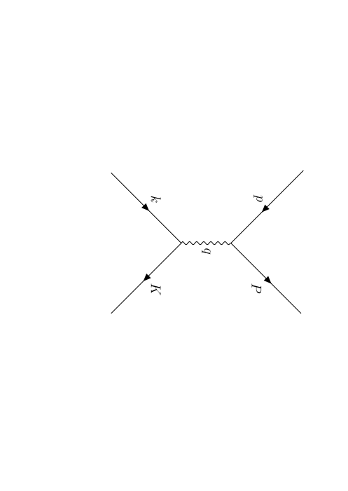
1P⟂2\displaystyle\frac{1}{P^{2}_{\perp}} =\displaystyle= 2s​[−32+limx0→111−x0]\displaystyle\frac{2}{s}\left[-\frac{3}{2}+\lim_{x_{0}\to 1}\frac{1}{1-x_{0}}\right]
=\displaystyle= 2s​[−32+limcos⁡θ0→111−cos⁡θ0],\displaystyle\frac{2}{s}\left[-\frac{3}{2}+\lim_{\cos\theta_{0}\to 1}\frac{1}{1-\cos\theta_{0}}\right],
1ϵB2\displaystyle\frac{1}{\epsilon^{2}_{B}} =\displaystyle= 2s​[−32+1ϵV],\displaystyle\frac{2}{s}\left[-\frac{3}{2}+\frac{1}{\epsilon_{V}}\right],
o​r\displaystyle or
1ϵV\displaystyle\frac{1}{\epsilon_{V}} =\displaystyle= s2​ϵB2+32,\displaystyle\frac{s}{2\epsilon_{B}^{2}}+\frac{3}{2},

where ϵB\epsilon_{B} is the lower cut off on P⟂P_{\perp} and ϵV=1−cos⁡θ0\epsilon_{V}=1-\cos\theta_{0}.