A Nonparametric Bayesian Method for Clustering of High-dimensional Mixed Dataset
Abstract
Motivation: Advances in next-generation sequencing (NGS) methods have enabled researchers and agencies to collect a wide variety of sequencing data across multiple platforms. The motivation behind such an exercise is to analyze these datasets jointly, in order to gain insights into disease prognosis, treatment, and cure. Clustering of such datasets, can provide much needed insight into biological associations. However, the differing scale, and the heterogeneity of the mixed dataset is hurdle for such analyses.
Results: The paper proposes a nonparameteric Bayesian approach called Gen-VariScan for biclustering of high-dimensional mixed data. Generalized Linear Models (GLM), and latent variable approaches are utilized to integrate mixed dataset. Sparsity inducing property of Poisson Dirichlet Process (PDP) is used to identify a lower dimensional structure of mixed covariates. We apply our method to Glioblastoma Multiforme (GBM) cancer dataset. We show that cluster detection is aposteriori consistent, as number of covariates and subject grows. As a byproduct, we derive a working value approach to perform beta regression.
Keywords: Nonparametric Bayes; Dirichlet process; Poisson Dirichlet process; Mixed data clustering; Biclustering; Beta regression; Generalized Linear Model
1 Introduction
Technological advances in next-generation sequencing (NGS) methods have facilitated researchers to sequence DNA at an unprecedented speed. This has led to proliferation of high resolution genomic data such as transcriptomic data (e.g mRNA expression), epigenomic data (e.g DNA methylation) etc. For instance, The Cancer Genome Atlas (TCGA) has compiled large genomic databases for different tumor types. These databases are sourced from multiple genomic platforms on a common set of samples, and are of different data types. Each of these datasets provide a partly independent and complementary view of the genome (Hamid et al., 2009).
A problem of interest in integrative genomics is to analyze these datasets jointly. Specifically, there is a considerable interest in studying biological associations across data types. Biological associations play a crucial role in tumor growth, and studying these interactions can provide for a comprehensive understanding of cancer genetics and molecular biology (Lock and Dunson, 2013). Clustering, an unsupervised approach to group objects into clusters which share common pattern, is often used to find biological associations. Eisen et al. (1998) first, applied clustering methods to find associations among genes in gene expression data. Since then, clustering methods have been employed to find biological associations. Recently, clustering technique has been applied to discover interactions between biomarkers of continuous (gene expression) and categorical data type (DNA copy number alteration / DNA mutation) (Lee et al. (2008), Abidin and Westhead (2017)).
An open problem, in this context, is to perform biclustering or two-way clustering of high-dimensional mixed datasets. The advantage of biclustering approach over one-dimensional clustering approach is that clustering is done simultaneously between samples and covariates. In biological context, it means that there may be a group of biomarkers (across data types) that defines the biological process for only a subset of samples (Lee et al., 2013). In other words, a biclustering approach borrows strength from local interactions. Several studies have established biological relevance of biclustering methods (Oghabian et al., 2014). Despite the advantages of biclustering methods, we lack a biclustering method for high-dimensional mixed dataset. In this paper, we propose a biclustering method for integrating high-dimensional mixed dataset with an emphasis on clustering the covariates.
1.1 Challenges in high dimensional mixed data
The challenge with high dimensional mixed dataset is two fold. The dataset is heterogeneous and consists of multiple data types (such as continuous, binary etc). It is difficult to combine the information across different data types in a meaningful manner as each data type is on a different scale. Moreover, for biomedical mixed datasets, the number of subjects are relatively small compared to the number of covariates (n p). Therefore, one needs to reduce the number of covariates to a smaller number of covariates for subsequent analyses.
1.2 Current Approaches and its limitations
There’s an extensive literature for clustering of high dimensional mixed datasets. The popular approaches include K-means/K-mediods algorithm using Gower’s distance and hierarchical clustering approaches. Over the years, a number of methods have been developed for clustering of high-dimensional mixed dataset with a focus on clustering the samples. For a detailed review, see Wei (2015) and Huang et al. (2017). Broadly, these methods could be classified as i) Matrix Factorization method, and ii) Model based clustering method.
Matrix Factorization: Matrix factorization based approaches makes use of the fact that the data matrix can be written in terms of sparse latent factor matrix. Shen et al. (2009) developed a latent factor approach for integrating multiple datasets of different data types. Mo et al. (2013) generalized Shen et al. (2009)’s approach for binary, multicategory, and continuous data types. Lock et al. (2013) proposed a latent factor approach (JIVE), where they decomposed the total variation into joint variation and individual variation. The limitations of above approaches are that they require normalization across datasets, and assume a linear mapping between the data points and latent factors.
Model based clustering: Model based clustering approaches relaxes the linearity assumption between the latent factors and data point. They incorporate likelihood of data points, and use non-parametric Bayesian method to cluster data points into different groups. Savage et al. (2010) proposed a modified version of Hierarchical Dirichlet Process (HDP) (Teh et al., 2006) to jointly model gene-expression and transcription factor binding data. Kirk et al. (2012) proposed a general approach to integrate multiple data types, simultaneously. Lock and Dunson (2013) proposed a Bayesian consensus clustering approach. They made use of finite Dirichlet Mixture Models to model each dataset separately. The limitation of above approaches are that it is computationally difficult and expensive for non-normal likelihoods, or where conjugacy can’t be easily exploited.
Existing methods in integrative genomics have only been used to identify the subtype or cluster among the patients (or subjects). The other limitation of existing methods is that they do not allow for biclustering (simultaneous) clustering of samples and covariates. With an aim to overcome above limitations, we propose a nested partition model for high-dimensional mixed dataset.
1.3 Nested Partition Models
Product Partition models were first studied by Barry and Hartigan (1992). Quintana and Iglesias (2003) and Quintana (2006) defined product partition models in a nonparametric Bayesian set up. Let be a data matrix, where each row denotes a sample and each column denotes a covariate. Then, the product partition model in a nonparametric Bayesian set up, can be given as below.
| (1) |
where is a parameter, is a hyperparameter, M is concentration parameter, G is a mixing distribution, and RPM is a random probability measure.
The mixing distribution G is almost surely discrete which facilitates the observations to group into clusters and share common ’s. This allows one to naturally infer the number of clusters. Also, the random partition model is exchangeable under the permutation of cluster indices (Müller et al., 2011).
The product partition models could be generalized to nested partition models. Recently, many authors have proposed such models (for e.g Rodriguez et al. (2008), Rodriguez and Ghosh (2012), Lee et al. (2013)). In nested partition models, the data matrix ( ) are clustered at two levels, which allows the model to borrow strength from local interactions. Lee et al. (2013) proposed a nonparameteric Bayesian model for clustering of RRPA data. They proposed nested clustering of covariates using Dirichlet Process (DP) both at column and row level. Guha and Baladandayuthapani (2016) argued that nested Dirichlet Process (DP) with Poisson Dirichlet Process (PDP) leads to more flexible clustering. They applied their method to gene expression data. Xu et al. (2013) modified Lee et al. (2013)’s biclustering approach for histone modification data. Reverse Phase Protein Array data, gene expression data, and histone modification data are continuous, continuous, and count data respectively. A limitation of above methods is that they can’t be applied to a mixed dataset, consisting of continuous and categorical data type. We fill this gap and extend Guha and Baladandayuthapani (2016)’s approach to mixed datasets.
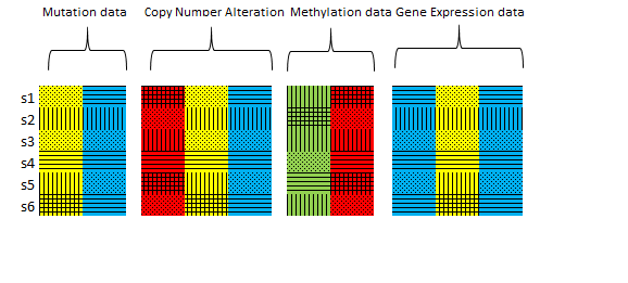
Gen-VariScan is a clustering method which biclusters (simultaneously clusters) mixed data matrix . The method can be described in two steps, namely:- i) regression step, ii) clustering step. We start with an initial cluster label for every element in the data matrix. In regression step, we perform regression analysis for every column vector where the dependent variable is original column vector and the independent variables are cluster label vector. The regression method depends on data type of the column vector, see Figure 1. The coefficient of cluster label vector is a latent vector, which is continuous. In clustering step, the latent vectors are clustered to q () PDP clusters. Subsequently, the unique elements of all latent vectors ( are clustered using DP. It is worth noting that one can easily cluster the continuous latent vector, in comparison to, the original column vector (which can be continuous/ discrete). Here, the biclustering of (continuous) latent vectors is used as proxy for biclustering of mixed dataset. Moreover, for latent variable approaches (Albert and Chib (1993)) and GLM (McCullagh and Nelder (1989)), the latent continuous vector is approximately normal. This allows us to use conjugacy properties and gain computational efficiency (see Section 3). The column intercept is used to center each covariate column (across data type). Figure 2 illustrates our method. There are 4 datasets of different data types namely:- mutation, copy number alteration, methylation, and gene expression datasets. In total, there are n= 6 samples, and p=10 covariates. Clusters of individual cells are denoted by pattern and column level clusters are encoded by colors.
Gen-VariScan has following advantages over other integrative approaches. It doesn’t normalize the datasets and therefore can effectively capture heterogeneity in the datasets. It borrows strength from local clustering, which leads to more flexible clustering. It is computationally efficient as it exploits the conjugacy between the density of latent variable and the base distribution of DP. The main contribution of this paper are as follows:- 1) We extend Guha and Baladandayuthapani (2016)’s approach to mixed datasets, 2) We prove that cluster allocation is aposteriori consistent, 3) As a byproduct, we derive a working value approach for beta regression.
We have drawn motivation for our model from high through-put biomedical set up but our method can be used elsewhere to perform i) data integration, ii) biclustering (simultaneous clustering) of mixed datasets, iii) dimension reduction. The rest of the paper is organized as follows. In Section 2, we propose a working value approach to do beta regression which is used subsequently in biclustering of mixed dataset. In Section 3, we describe our model. In Section 4, we describe posterior inference for implementing our model. In Section 5, we discuss methods to evaluate our model. In Section 6, we perform simulation analyses of the model. In Section 7, we apply the model on a real dataset and discuss the results. Section 8 summarizes our paper. Supplementary materials contain the theorem proofs, as well as additional data analysis results.
2 Beta Regression
Beta regression has received considerable attention in recent years. Ferrari and Cribari-Neto (2004) reparametrized beta density and proposed a classic beta regression model for constant dispersion parameter. Branscum et al. (2007) proposed Bayesian beta regression. Simas et al. (2010) proposed a generalized model where the dispersion parameter is not constant. Figueroa-ZunIga et al. (2013) proposed mixed beta regression. The limitation with above approaches is that they can’t be readily used in an ensemble set up (such as ours), where one borrows strength from multiple models. A workaround would be to find a working value approach for beta regression (McCullagh and Nelder, 1989). Recently, Cepeda-Cuervo et al. (2016) proposed a working value based approach for Bayesian beta regression. However, their approach isn’t numerically stable. We explain this later in the section. But, first, let us define beta density.
2.1 Beta Density
A random variable y, follows a beta distribution, whose probability density function is given as below.
where are shape parameters and . Ferrari and Cribari-Neto (2004) suggested a reparameterization of the beta density in terms of (the mean parameter) and (the dispersion parameter).
The reparametrized beta density is given as below.
| (2) |
where are mean and disperson parameter, respectively.
Cepeda-Cuervo et al. (2016) made use of working variable approach which is commonly carried out to implement Generalized Linear Models (GLM), for details see (McCullagh and Nelder, 1989). Their proposed working value is given as below.
| (3) |
where y denotes observation, denotes working value, x denotes the covariates for regression, and denote the current value of and (coefficients) respectively. The limitation of above approach is that it doesn’t work well when is moderately close to 0 or 1. The gradient diverges and therefore working value approach becomes numerically unstable, see Figure 3.
2.2 Proposed Beta Regression
Let follow beta distribution. Let be the covariates and denotes the coefficients. Also, let denotes the mean of for i = and, the link function be given as below.
| (4) |
where g is the link function.
The link function g, maps from [0,1] R. There are a number of choice for link functions, for example , where F is any cumulative distribution function. One may also specify the link function as the complementary log link , the log-log link among others. We specify the link function as below.
| (5) |
The above link function has a natural interpretation in terms of odds ratio. For detailed discussion on link functions, see McCullagh and Nelder (1989).
Theorem 2.1
The score function for the reparametrized beta density is given as
| (6) |
Furthermore, the score function satisfies following regularity conditions :-
| (7) |
where b denotes the current estimate of and denotes the adjustment.
Then, the working value for beta regression is given as
| (8) |
where , , denotes digamma function, denotes trigamma function, and A is the fisher’s information matrix (.
In Appendix A.1 .
Fact 2.2
The gradient of working value proposed in Theorem 2.1 is bounded from above, and the upper bound is given as below
| (9) |
In Appendix A.2.
Theorem 2.1 gives the working value for beta regression. Figure 4 and Fact 2.2 show that the gradient in Theorem 8 is bounded. Further, the approximate density of z is given as below.
| (10) |
where denotes the trigamma function.
In this section, we proposed a working value approach for beta regression. Our working value approach could be used in any other settings to perform Bayesian beta regression. We use above result in proposing a nonparameteric Bayesian model for mixed datasets, which includes proportion data.
3 Model
Suppose we take continuous, binary, ordinal, count, and proportion measurements on p biomarkers on n patients. These measurements can be organized in a data matrix X, with n rows and p columns (n p), where each row is a sample and each column a covariate. Further, we assume that each covariate belongs to one of the five data types, namely:- binary, ordinal, count, proportion, and continuous data type.
Gen-VariScan consists of three steps i) Allocation Variable ii) Latent Vectors iii) Data Augmentation. Figure 5 gives the visual representation of the model.
3.1 Allocation Variable
Let denote the set of p covariates, where , the covariate vector denotes measurement taken on n patients. A partition of set S yields q disjoint subsets: , such that , and . Let denote the cluster membership of to , i.e, means cluster, , . We refer to as allocation variable, where j= .
Following Guha and Baladandayuthapani (2016), we put a two parameter Poisson Dirichlet Process prior (PDP) on allocation variable, where discount parameter and precision or mass paramter . Perman et al. (1992) introduced PDP and later Pitman (1995), Pitman and Yor (1997) studied it further. Further, PDP and DP priors were generalized as Gibbs-type priors in Gnedin and Pitman (2005).
Guha and Baladandayuthapani (2016) gave theoretical and empirical justifications for putting PDP prior. The case for PDP prior can be made as follows. i) DP prior is a specific case of PDP prior (when d =0). ii) A PDP prior has sparsity inducing property which effectively reduces the number of cluster. Asymptotically, the number of cluster for PDP and DP prior can be given as below, see Guha and Baladandayuthapani (2016).
where as .
Since, the PDP assumes exchangability therefore the allocation labels are arbitrary. Without loss of generality, we could assign first covariate () into first cluster, i.e, . Thereafter, let’s say for j =2, , p covariate we have number of unique clusters among where cluster contains number of covariates. Then the conditional probability that covariate is assigned to cluster is
| (11) |
The PDP discount parameter d is given the mixture prior , where denotes the point mass at 0. Posterior inferences of d allows us to select between Dirichlet Process and PDP, which allows for flexible clustering.
3.2 Latent Vectors
Let denote the column vector with elements , where and is number of column clusters. We put a prior on the latent vectors , i.e, , where specifies a distribution in . Following Guha and Baladandayuthapani (2016), we write as n-fold product measure of univariate distribution. This essentially imposes a lower dimensional structure on ’s. Further, the prior helps us create nested clustering of subjects within covariates, which can capture local clustering and borrow strength across samples (patients) and covariates (biomarkers).
| (12) |
The unknown density is given a Dirichlet Process prior
| (13) |
where the mass parameter M 0 and the base distribution as a univariate normal distribution N(, ).
3.3 Data Augmentation
Posterior sampling in discrete regression models can be computationally challenging. Albert and Chib (1993) implemented data augmentation approach for binary and ordinal regression. Bayesian approaches in generalized linear models (GLM) makes use of working value approaches, see Dey et al. (2000), Guha (2008). Recently, nonparameteric Bayesian methods along with GLM and data augmentation approaches are used for discrete regression models. Messan et al. (2003) studied nonparametric Bayesian methods for binary regression. Hannah et al. (2011) used GLM with Dirichlet Process (DP) for regression. DeYoreo and Kottas (2017) used latent variable approch in nonparametric Bayesian setup for ordinal regression.
We introduce a latent vector vector correspond to every covariate vector . We define for cases, where belongs to one of the five data types, namely:- binary, ordinal, count, proportion and, continuous. For simplifying notations, we specify , denotes the estimated number of column cluster and denotes the true number of column cluster, for all the five data types.
;
Binary Data
We assume binary datapoint, to have an underlying likelihood, which is given below.
| (14) |
where is true cluster allocation, denote true latent vector element.
Following Albert and Chib (1993), we generate a latent variable , as follows.
| (15) |
where is column intercept, is estimated latent vector element, is estimated allocation variable.
Equation (15) isn’t identifiable. A simple workaround the identifiability problem is to fix . Note that we are interested in finding a group of biomarkers, which are similar in the sense of correlation/concordance. Therefore, fixing as column intercept doesn’t affect our analysis. A reasonable choice of can be given as below.
where .
Ordinal Data
We assume ordinal datapoint , to be distributed as follows.
| (16) |
where ’s are true cut offs, is true cluster allocation, denote true latent vector element.
Following Albert and Chib (1993), we generate a latent variable as follows.
| (17) |
where is column intercept, is estimated latent vector element, is estimated allocation variable, and q is estimated number of column cluster and ’s are estimated cut offs.
Like in binary case, equation (17) has identifiability problem. We approximate as column center, which is given as follows.
where .
We fix , , and to address identifiabiity concerns. The conditional distribution of is uniform in the interval .
Count Data
We assume count datapoint , to be distributed as follows.
| (18) |
where is true cluster allocation, denote true latent vector element, and indicate the number of true column clusters.
Then for log(.) link function, the adjusted dependent variable and it’s approximate density is given as below :-
| (19) |
where is column intercept, is latent vector element, is allocation variable.
Since, isn’t identifiable in equation (19), we fix as approximate center of column, we fix as below.
where .
Continuous Data
We assume continuous data point , to be distributed as follows.
| (20) |
where is true cluster allocation, denote true latent vector element, is true standard deviation, and is common intercept.
The latent variable is given by whose approximate density is given as under.
| (21) |
where is the column intercept, is estimated latent vector element, is estimated allocation variable, is estimated variance.
In order to address the identifiability problem in equation (21), we constraint that to be 0.
Proportion Data
We assume that proportion data point , to be distributed as follows.
| (22) |
where is true cluster allocation, denote true latent vector element, and is a constant for proportion data.
Under the log odds link function and using Theorem 2.1, the latent variable () and it’s approximate density can be given as follows :-
| (23) | |||||
where , , denotes digamma function, and denotes trigamma function, is column center, is estimated dispersion, is estimated cluster allocation, is estimated latent vector element, and indicates estimated number of column clusters.
We specify the following prior on
where refers to Gamma density.
In order to address identifiability problem in equation (23), we constraint that to make it identifiable.
4 Posterior Inference
Posterior inference is computationally expensive. We apply Guha (2010)’s data squashing algorithm to speed up computation. We start with an initial configuration of the model parameters. The model parameters are iteratively updated by the MCMC procedure. Broadly, the MCMC procedure can be divided into two steps.
- 1.
Conditional on the current model parameters, we update the data augmentation variable for each of five data types. Subsequently, we update the allocation variable, latent vector elements, and hyperparameters until the MCMC chain converges. See Appendix A.2 for further details.
- 2.
We compute Monte Carlo estimates to compute the posterior probability of clustering for each pair of covariates. Dahl (2006) proposed a method which uses pairwise probabilities to get the point estimate of binary vector, which is called the least-square allocation. At the end of MCMC iteration, we use Dahl (2006) to estimate the least-square allocation.
5 Clustering Consistency
Clustering consistency, may seem like a desireable property for clustering procedure, but it is hardly guaranteed. Müller et al. (2011) notes that the random partition models are exchangeable under permutations and hence, actual clusters and cluster related inferences are subject to label switching problem, as in finite mixture models. Clustering under finite mixture models often results in non-identifiablity, and redundancy in clusters (see, Fruhwirth-Schnatter (2006)). Rousseau and Mengersen (2011) showed that a careful choice of priors yields emptied redundant clusters for over-fitted mixture models. Petralia et al. (2012) defined a repulsive process, which leads to better separated clusters. The general strategy of above solutions is to impose identifiability constraints and detect the true number of clusters. However, above methods fall short of discovering the true allocation of objects into clusters.
Like finite mixture models, non-parameteric Bayesian models doesn’t guarantee cluster consistency, until very recently.
In a surprising result, Guha and Baladandayuthapani (2016) proposed a biclustering model for clustering continuous data matrix with n rows and p columns. As n (sample size) and p (covariates) becomes large, they showed that their model can discover true cluster allocation of p covariates. The intuition behind this phenomenon is that as n and p becomes large the n-dimensional objects becomes well separated in and form identifiable clusters. Theorem 5.1 extends Guha and Baladandayuthapani (2016)’s result on clustering consistency to mixed dataset.
True model. Let be a mixed dataset, where belong to one of the five data types, namely:- binary, continuous, count, ordinal, and proportion. Let denote the sample space for , where indicate the data type of Let be the probability density function on the space which is defined in Definition 5.1. Further, we make the following assumptions about the covariate generating process.
- 1.
The elements of data matrix, , are independent, but not identical realizations, from a true mixing distribution convoluted with some exponential family densities, which are given in Definition 5.1,
- 2.
The true mixing distribution is discrete in , which implies that the true n-variate mixing distribution is discrete, as well. The discreteness of implies the existence of true cluster allocation variable ,
- 3.
where , , is the number of true clusters, and is given in Definition 5.1,
- 4.
The atoms of are i.i.d realizations of a univariate normal distribution, .
Definition 5.1
where, denotes the cdf of standard normal distribution, denotes the standard normal density, denote the cut off points for the ordinal data, ).
Let be a fixed subset of L covariate index. true allocation variable be denoted by for j = and the estimated allocation variable be denoted by for j = , then we compute the allocation accuracy by mean-taxicab distance between and , which is given below.
A low value of (e.g 0) indicates low accuracy and a high value of (e.g 1) indicates high accuracy for estimated allocation vector c for the set . It is worth noting that is invariant of the permutation of the cluster labels.
Theorem 5.1
Let be a mixed dataset, where belong to one of the five data types, namely :- binary, continuous, count, ordinal, and proportion. In addition to the model assumptions (1)-(3), we assume that in (3) is bounded, i = .
Let be a fixed subset of L covariate index. Then, there exists an increasing sequence , that grows with n provided , and the clustering inferences for the covariate subset are aposteriori consistent. That is,
See Appendix A.4 for the proof.
6 Simulation Studies
To evaluate the performance of Gen-VariScan procedure to detect covariate column clusters, we study artificially simulated datasets under different scenarios. The parameters of true model were chosen to closely match the estimates of the benchmark data analysis. We also perform a comparison against other methods, when true column clusters are known.
6.1 Simulation scheme
We investigate the proposed method’s accuracy as a clustering procedure for mixed datasets using artificial dataset for which true clustering pattern is known. The artificial data was selected to have the same dimension as benchmark dataset (n =71 subjects and p =352 covariates), and then we compared the co-clustering probabilities of p covariates against truth. The simulation analysis was done for different mix of mixed dataset, including one which closely resembles the mix of benchmark data. Depending on the mix of the data, the artificial data was simulated as below.
- 1.
True Allocation variables: We generate as partitions through Poisson Dirichlet Process (PDP) with a discount parameter d = 0.3 and mass parameter . Thereby, we compute the true number of clusters .
- 2.
Latent vector elements : For i = 1, , n , k = 1, , elements , where with mass parameter = 11 and base distribution . We choose , and .
- 3.
Covariates : For each covariate column, we assign a data type out of five data types (binary, ordinal, count, continuous, and proportion) using multinomial distribution with a pre-specified probability according to the mix of dataset. Subsequently, we simulate the covariate column. For each data type, the covariate column is generated using a density function, which is a function of two components i) ii) , where . Specifically, we generate the element of covariate column as below ().
- •
Binary :
- •
Continuous : where , .
- •
Count : .
- •
Ordinal : The ordinal data points were assumed to have five categories.
where - •
Proportion :
where .
- •
6.2 Comparison
The artificial data was simulated as per the settings in section 6.1 for seven different scenarios. The scenarios depend on the mix of data type in the dataset. Five scenarios corresponds to five data types, benchmark data mix scenarios resembles mix of data type in the benchmark data, and uniformly mix of data type across five data types. Further, the comparison study was replicated 15 times. For each dataset, we ran the simulation for 15,000 iterations, where we ignored the first 5,000 iterations as burn-in. Subsequently, using Dahl (2006), we estimated a point estimate for cluster allocations, called the least-squared configuration, and denoted by . Finally, we estimated the accuracy of our method by estimating the proportion of correctly predicted clustered covariate pairs, , which is given below.
A high value of (e.g 1) or a low value of (e.g 0) indicates high clustering accuracy. We evaluate our method against Partition around mediods (PAM) with gower’s distance (Maechler et al., 2018), and ClustOfVar’s hierarchical clustering approach (Chavent et al., 2012). The number of cluster for PAM and ClustOfVar was estimated using maximum silhoutte width. For each of the dataset, we ran the MCMC for 15,000 iterations where the first 5,000 iteration was discarded as burn in. Using Dahl (2006) we computed a point estimate for cluster allocations. Subsequently, we evaluated the three method by computing the proportion of incorrectly predicted clustered covariate pairs, .
Figure 6 gives the boxplot of error ( ) for each of the three methods for seven different scenarios. The figure further shows that PAM and ClustOfVar fairs marginally better than Gen-Variscan when the covariates consists of a single data type. The accuracy of PAM and ClustOfVar could be attributed to the phenomenon that objects in tends to become well separated for large n (see Section 5). PAM and ClustOfVar can detect these well separated objects when datasets consists of single data type. However, the figure shows that PAM and ClustOfVar are highly inaccurate for mixed data scenarios whereas Gen-Variscan maintains a consistency in accuracy across different mix of data types. This shows that Gen-Variscan is well-suited to cluster mixed datsets, in comparison to other two methods. The boxplot (see Figure 6) shows that Gen-VariScan’s median error () of incorrectly classifiying covariate pairs is atmost about 0.02, across all scenarios. This suggests that Gen-VariScan correctly classifies about 60,886 covariate pairs out of and incorrectly classifies about 1,242 covariate pair out of total . It is worth pointing that Gen-Variscan’s accuracy is consistently across the scenarios.
Table 1 gives the 95 % credible interval for the lower bound of the Bayes Factor of a PDP model and a DP model. The lower bound of the Bayes Factor is given by . Besides 100 % count and 100 % binary, we find overwhelming evidence in favor for the PDP model against DP model. This is true even though we had a put a prior . For 100 % binary scenario, there’s a strong evidence in favor of the PDP model, but it’s inconclusive in case of 100 % count scenario. The table also gives the 95 % credible interval for the estimated d. We note that the true value of d, i.e 0.3, lie within the 95 % credible interval for all the scenario. This validates that our model can estimate true level of sparsity among column clusters.
| Estimated d | log Bayes Factor | |||
|---|---|---|---|---|
| Scenario | Lower C.I | Upper C.I | Lower C.I | Upper C.I |
| Benchmark Data Mix | 0.200 | 0.401 | Inf | Inf |
| Uniformly Mix Data | 0.262 | 0.484 | Inf | Inf |
| 100% binary | 0.078 | 0.399 | 0.974 | Inf |
| 100% continuous | 0.229 | 0.547 | Inf | Inf |
| 100% count | 0.00 | 0.32 | -1.77 | Inf |
| 100% ordinal | 0.274 | 0.386 | Inf | Inf |
| 100% proportion | 0.183 | 0.462 | 6.87 | Inf |
We also evaluate the model for different value of (standard deviation for continuous data), (dispersion parameter proportion data) for the benchmark data mix scenario. Table 2 gives the 95 % credible interval for d for benchmark data mix. We see that the true value of d, i.e 0.3, lies within the credible interval. This reflects that our model can achieve similar level of sparsity as the true model, which further validates our method.
| Scenario | 95 % C. l of d | ||
|---|---|---|---|
| Lower | Upper | ||
| 0.1 | 10 | 0.201 | 0.345 |
| 0.1 | 20 | 0.174 | 0.330 |
| 0.1 | 30 | 0.175 | 0.332 |
| 0.5 | 10 | 0.292 | 0.439 |
| 0.5 | 20 | 0.148 | 0.311 |
| 0.5 | 30 | 0.284 | 0.436 |
| 0.9 | 10 | 0.160 | 0.317 |
| 0.9 | 20 | 0.298 | 0.450 |
| 0.9 | 30 | 0.241 | 0.374 |
7 Benchmark Data Analysis
7.1 Data Description
We downloaded TCGA Glioblastoma Multiforme (GBM) dataset through TCGA2STAT package in R (Ying-Wooi et al., 2015), which includes gene expression, copy number alteration, methylation, and mutation datasets. Each of these datasets is extracted from a different platform. The gene expression dataset comes from Affymetrix Human Genome U133A 2.0 Array, the methylation dataset comes from Illumina Infinium HumanMethylation27, the copy number alteration comes from Affymetrix SNP6, and the mutation data was obtained from Mutation Annotation Format (MAF). The gene expression and the mutation dataset is at the gene level (level 3), whereas the copy number alteration and methylation dataset was obtained at probe level (level 2) and then mapped to the gene level (level 3).
Each dataset has 10 normal samples. For gene expression and copy number alteration biomarkers, we used Wilcoxon rank sum test to determine whether or not biomarkers were different between the tumor case and the normal sample. A p-value threshold () was applied to select the biomarkers. We filtered the mutation biomarkers, which had less than 10 number of mutation occurences. Further, we included gene expression, copy number alteration, methylation, and mutation of genes which comprises the RB pathway, RTK/Ras/PI3K/AKT pathway, and TP53 pathway. These pathways are associated with Glioblastoma cancer (TCGA, 2008). We merged the datasets by patient and kept the patient records which were present in all the four data types. The combined dataset consists of 71 patients and 352 covariates.
7.2 Results
We analyzed the merged dataset (GBM data) using our method. Figure 7 gives the posterior summary of q (number of clusters) and d (discount parameter). The estimated number of covariate cluster turned out to be = 70.
Figure 8 shows that majority of the covariates are allocated into a fewer clusters of moderate/large size, and a large number of smaller clusters. This is similar to sparsity structure imposed by clustering under PDP process. The bargraph also gives a visual insight into shared cluster membership of covariates across data types. The bargraph color codes the proportion covariate as blue, ordinal covariates as green, continuous covariates as yellow, and binary covariates as cyan. It is worth noting that the common denominator in majority of the shared clusters (across data types) is continuous data type, which corresponds to the gene expression data. The existing knowledge of biological mechanism confirms this finding, and moreover it shows that the above covariate partition captures useful biological information (Savage et al., 2010). Finally, we see there are non-singleton clusters which are of the same data type. This phenomenon is confirmed by the existing knowledge of system biology, see (Wenting et al., 2013).
The effectiveness of our model could be further demonstrated as follows. For each of the estimated non-singleton covariate clusters, we compute the correlation between its member covariates in the original data. The median correlation gives a summary of associations in these clusters. The median correlations of estimated covariate clusters are plotted in Figure 9. We note that the median correlations are all positive. This strongly suggests that our method has found groups of biomarkers which share a similar pattern in the original dataset. We also plot the median correlation against the cluster size in Figure 9, which confirms that the median correlation of estimated clusters is moderate despite the cluster size.
Furthermore, we looked at the transformed covariates which were allocated into covariate clusters with more than 10 covariates (biomarkers). We compared the heatmap of such transformed covariates with the heatmap of corresponding original covariates in Figure 10. The gain from our method is apparent, as the heatmap of transformed covariates is comparatively even, whereas the heatmap of the original covariates is stark, in comparison. We also partition the heatmap of the transformed covariate into different clusters on the basis of estimated cluster membership, using solid black lines, see Figure 10. We note that the heatmap of the transformed covariates within a cluster is quite similar.
For biological relevance of our findings, we looked up biomarkers on the same gene which share the estimated cluster. This could explain the role of biological association on same gene (across data type) play in tumor growth. Subsequently, we verified our findings about these genes and their interactions by cross-referencing them in cancer literature. We found that genes associated with GBM cancer were mutated, amplified or methylated to have a positive associated with gene expression. For instance, copy number alteration of EGFR (Xu, 2014), MDM4 (Furgason et al., 2015), mutation of TP53 gene (Verhaak, 2010), and methylation of CKDN2B gene (Kazanets, 2016) and PTEN gene (Baeza, 2003) at certain sites were associated with corresponding gene expression on respective genes. We corroborated these findings by looking up in the cancer literature. Our findings gives us an insight into the underlying biology and how these associations play a part in tumor growth. A detailed analysis of the mechanistic interpretation of these genes is given in Appendix A.5.
8 Conclusion/Discussion
Using data augmentation approach, we extended Guha and Baladandayuthapani (2016)’s approach to mixed datasets. Gen-VariScan is a flexible technique for clustering of high-dimensional mixed datasets. It groups mixed covariates into small number of clusters, which consists of similar covariates. We provide theoretical justification for the data augmentation approach, and also prove that our method can detect true co-clustering of covariates. We also demonstrate the effectiveness of our model through simulation and real data analysis. The proposed method outperforms existing approaches for the mixed dataset. In real data analysis, we identified several biological association and interaction, which has known implications in development and progression of cancer. As a byproduct of our work, we also propose a working value approach for beta regression for constant dispersion.
Potentially, one could use our approach to perform survival regression, or find subtypes among patients. It would be worth investigating the gains from such an approach. Another area of investigation is to study the convergence rates of the co-clustering of covariates. The convergence rate can help us foresee the performance of our method on a large dataset. Finally, our beta regression approach can be used in other settings.
Supplementary Material
Supplementary material includes additional details on workings of Gen-VariScan, biological interpretations of Benchmark Data Analysis, and proofs of theorems.
References
- Abidin and Westhead (2017) Faitin N. Zainul Abidin and David R. Westhead. Flexible model-based clustering of mixed binary and continuous data : application to genetic regulation and cancer. Nucleic Acids Research, 45(7):e53, 2017.
- Albert and Chib (1993) James H. Albert and Siddhartha Chib. Bayesian analysis of binary and polychotomous response data. Journal of the American Statistical Association, pages 669–679, 1993.
- Baeza (2003) N et al. Baeza. Pten methylation and expression in glioblastomas. Acta Neuropatholica, 106(5):479–85, 2003.
- Barry and Hartigan (1992) Daniel Barry and J. A. Hartigan. Product partition models for change point problems. Annals of Statistics, 20(1):260–279, 1992.
- Branscum et al. (2007) Adam J. Branscum, Wesley O. Johnson, and Mark C. Thurmound. Bayesian beta regression : Applications to household expenditure data and genetic distance between foot-and-mouth disease viruses. Austrailian and New Zealand Journal of Statistics, 49(3):287–301, 2007.
- Cepeda-Cuervo et al. (2016) Edilberto Cepeda-Cuervo, Jaimes Daniel, Marin Margarita, and Rojas Javier. Bayesian beta regression with bayesianbetareg r-package. Computational Statistics, 31:165–187, 2016.
- Chavent et al. (2012) M. Chavent, V. Kuentz-Simonet, B. Liquet, and J. Saracco. Clustofvar : An r package for the clustering of variables. Journal of Statistical Software, 50(13):1–16, 2012.
- Dahl (2006) D. B. Dahl. Model-Based Clustering for Expression Data via a Dirichlet Process Mixture Model. Cambridge University Press, 2006.
- Dey et al. (2000) Dipak K. Dey, Sujit K. Ghosh, and Bani K. Mallick. Generalized Linear Models: A Bayesian Perspective. CRC Press, 2000.
- DeYoreo and Kottas (2017) Maria DeYoreo and Anthanasios Kottas. Bayesian nonparametric modeling for multivariate ordinal regression. Journal of Computational and Graphical Statistics, pages 1–14, 2017.
- Eisen et al. (1998) Michael B. Eisen, Paul T. Spellman, Patrick O. Brown, and David Botstein. Cluster analysis and display of genome-wide expression patterns. Proceedings of National Academia of Science, USA, 95(25):14863–14868, December 1998.
- Ferrari and Cribari-Neto (2004) Silvia Ferrari and Fracisco Cribari-Neto. Beta regression for modelling rates and proportions. Journal of Applied Statistics, 31(7):799–815, 2004.
- Figueroa-ZunIga et al. (2013) Jorge I. Figueroa-ZunIga, Reinaldo B. Arellano-Valle, and Silvia L. P. Ferrari. Mixed beta regression : A bayesian perspective. Computational Statistics and Data Analysis, 61:137–147, 2013.
- Fruhwirth-Schnatter (2006) Sylvia Fruhwirth-Schnatter. Finite Mixture and Markov Switching Models. Springer, 2006.
- Furgason et al. (2015) JM Furgason, Koncar RF, Michelhaugh SK, Sarkar FH, Mittal S, Sloan AE, Barnholtz-Sloan JS, and Bahassi el M. Whole genome sequence analysis links chromothripsis to egfr, mdm2, mdm4, and cdk4 amplification in glioblastoma. Oncoscience, 2(7):618–28, 2015.
- Gnedin and Pitman (2005) A. Gnedin and J. Pitman. Exchangeable gibbs partitions and stirling triangles. Zap. Nauchn. Sem. S.-Peterburg. Otdel. Mat. Inst. Steklov. (POMI), 325:83–102, 2005.
- Guha (2008) Subharup Guha. Posterior simulation in the generalized linear mixed model with semiparametric random effects. Journal of Computational and Graphical Statistics, 17(2):410–425, 2008.
- Guha (2010) Subharup Guha. Posterior simulation in countable mixture models for large datasets. Journal of the American Statistical Association, 105(490):775–786, 2010.
- Guha and Baladandayuthapani (2016) Subharup Guha and Veerabhadran Baladandayuthapani. A nonparametric bayesian technique for high-dimensional regression. Electronic Journal of Statistics, 10:3374–3424, 2016.
- Hamid et al. (2009) Jemila S. Hamid et al. Data integration in genetics and genomics: Methods and challenges. Human Genomics and Proteomics, 2009.
- Hannah et al. (2011) Lauren A. Hannah, David M. Blei, and Warren B. Powell. Dirichlet process mixtures of generalized linear models. Journal of Machine Learning Research, 12(Jun):1923–1953, 2011.
- Huang et al. (2017) Siijia Huang, Kumardeep Chaudhary, and Lana X. Garmire. More is better: Recent progress in multi-omics data integration methods. Frontier in Genetics, 8(84), 2017.
- Kazanets (2016) Anna et al. Kazanets. Biochima et biophysica (bba)- reviews on cancer. 1865(2):275–288, 2016.
- Kirk et al. (2012) Paul Kirk, Jim E Griffin, Richard S. Savage, Zoubin Ghahramani, and David L Wild. Bayesian correlated clustering to integrate multiple datasets. Bioinformatics, 28(24):3290–3297, 2012.
- Lee et al. (2008) H Lee, Kong SW, and Park PJ. Integrative analysis reveals the direct and indirect interactions between dna copy number alterations and gene expression changes. Bioinformatics, 24(7):889–96, 2008.
- Lee et al. (2013) Juhee Lee, Peter Müller, Yitan Zhu, and Yuan Ji. A nonparametric bayesian model for local clustering with application to proteomics. Journal of the American Statistical Association, 108(503):775–788, 2013.
- Lock and Dunson (2013) Eric F. Lock and David B. Dunson. Bayesian consensus clustering. Bioinformatics, 29(20):2610–16, 2013.
- Lock et al. (2013) Eric F. Lock, Katherine A. Hoadley, J. S. Marron, and Andre B. Nobel. Joint and individual variation explained (jive) for integrated analysis of multiple data types. Annals of Applied Statistics, 7(1):523–542, 2013.
- Maechler et al. (2018) Martin Maechler, Peter Rousseeuw, and Anja Struyf. ”Finding Groups in Data”: Cluster Analysis Extended Rousseeuw et al. https://cran.r-project.org/web/packages/cluster/index.html, 2018. R package version 2.0.7.1.
- McCullagh and Nelder (1989) P. McCullagh and J. A. FRS Nelder. Generalized Linear Models. Springer, 2 edition, 1989.
- Messan et al. (2003) Amewou-Atisso Messan, Subhashis Ghoshal, K. Jayant Ghosh, and V. R. Ramamoorthi. Posterior consistency for semi-parametric regression problems. Bernoulli, 9(2):291–312, 2003.
- Mo et al. (2013) Q Mo et al. Pattern discovery and cancer gene identification in integrated cancer genomic data. Proceedings of the National Academy of Sciences of the United States of America, 110(11):4245–50, 2013.
- Müller et al. (2011) Peter Müller, Fernando Quintana, and Gary L. Rosner. A product partition model with regression on covariates. Journal of Computational and Graphical Statistics, 20(1):260–278, 2011.
- Oghabian et al. (2014) Ali Oghabian, Sami Kilpinen, Sampsa Hautaniemi, and Elena Czeizler. Biclutering methods : Biological relevance and application in gene expression analysis. PLoS One, 9(3):e90801, 2014.
- Perman et al. (1992) M Perman, J Pitman, and M Yor. Size-biased. Probability Theory and related fields, 92:21–39, 1992.
- Petralia et al. (2012) F. Petralia, V. Rao, and David Dunson. Repulsive mixtures. ArXiv e-prints, April 2012, 2012.
- Pitman (1995) Jim Pitman. Exchangeable and partially exchangeable random partitions. Probability Theory and related fields, 105:145–158, 1995.
- Pitman and Yor (1997) Jim Pitman and Marc Yor. The two-parameter poisson-dirichlet distribution dervied from a stable subordinator. The Annals of Probability, 25(2):855–900, 1997.
- Quintana (2006) Fernando A. Quintana. A predictive view of bayesian clustering. Journal of Statistical Planning and Inference, 136(8):2407–2429, 2006.
- Quintana and Iglesias (2003) Fernando A. Quintana and Pilar L. Iglesias. Bayesian clustering and product partition models. Journal of the Royal Statistical Society. Series B, 65(2):557–574, 2003.
- Rodriguez and Ghosh (2012) A Rodriguez and K. Ghosh. Modeling relational data using nested infinite relational models. Tech rep. Department of Applied Mathematics and Statistics, Univeristy of California; Santa Cruz, 2012.
- Rodriguez et al. (2008) A Rodriguez, B. David Dunson, and AE Gelfand. The nested dirichlet process. Journal of the American Statistical Association, 103(483):1131–1144, 2008.
- Rousseau and Mengersen (2011) Judith Rousseau and Kerrie Mengersen. Asymptotic behavior of the posterior distribution in overfitted mixture models. Journal of the Royal Statistical Society, Series B, 73(5):689–710, 2011.
- Roy and Teh (2009) D. M. Roy and YW. Teh. The mondrian process. Advances in Neural Information Processing Systems, 21:1377–1384, 2009.
- Savage et al. (2010) RS Savage, Z Ghahramani, JE Griffin, J. de la Cruz Bernard, and DL Wild. Discovering transcriptional modules by bayesian data integration. Bioinformatics, 26(12):i158–67, 2010.
- Shen et al. (2009) Ronglai Shen, B. Adam Olshen, and Marc Ladanyi. Integrative clustering of multiple genomic data types using a joint latent variable model with application to breast and lung cancer subtype analysis. Bioinformatics, 25(22):2906–2912, 2009.
- Simas et al. (2010) B. Alexandre Simas, Barreto-Souza Wagner, and Rocha Andrea V. Improved estimators for a general class of beta regression models. Computational Statistics and Data Analysis, 54(2):348–366, 2010.
- TCGA (2008) TCGA. Comprehensive genomic characterization defines glioblastoma genes and core pathways. Nature, 455(7216):1061–8, 2008.
- Teh et al. (2006) Yee Whye Teh, Michael I. Jordan, Matthew J. Beal, and David M. Blei. Hierarchical dirichlet process. Journal of the American Statistical Association, 101(476):1566–1581, 2006.
- Verhaak (2010) RG et.al Verhaak. Integrated genomic analysis identifies clinically relevant subtypes of glioblastoma characterized by abnormalities in pdgfra, idh1, egfr, and nf1. Cancer Cell., 17(1):98–110, 2010.
- Wei (2015) Yingying Wei. Integrative analyses of cancer data: A review from a statistical perspective. Cancer Informatics, 14(S2):173–181, 2015.
- Wenting et al. (2013) Wang Wenting et al. ibag:integrative bayesian analysis of high-dimensional multiplatform genomics data. Bioinformatics, 29(2):149–159, 2013.
- Xu (2014) Hongsheng et al. Xu. Epidermal growth factor receptor in glioblastoma. Oncology Letters, 14(1):512–16, 2014.
- Xu et al. (2013) Yanxun Xu et al. Nonparametric bayesian bi-clustering for next generation sequencing count data. Bayesian Analysis, 8(4):759–780, 2013.
- Ying-Wooi et al. (2015) Wan Ying-Wooi, I. Allen Genevera, L. Anderson Matthew, and Liu Zhandong. TCGA2STAT: Simple TCGA Data Access for Integrated Statistical Analysis in R. https://cran.r-project.org/web/packages/TCGA2STAT/index.html, 2015. R package version 1.2.
Acknowledgements
We would like to thank Dr Subharup Guha for sharing his work on Guha and Baladandayuthapani (2016), without which the current work wouldn’t have been possible. This project was partly supported by NSF Grant 1416948.