Matter Effect of Light Sterile Neutrino: An Exact Analytical Approach
Abstract
The light sterile neutrino, if it exists, will give additional contribution to matter effect when active neutrinos propagate through terrestrial matter. In the simplest 3+1 scheme, three more rotation angles and two more CP-violating phases in lepton mixing matrix make the interaction complicated formally. In this work, the exact analytical expressions for active neutrino oscillation probabilities in terrestrial matter, including sterile neutrino contribution, are derived. It is pointed out that this set of formulas contain information both in matter and in vacuum, and can be easily tuned by choosing related parameters. Based on the generic exact formulas, we present oscillation probabilities of typic medium and long baseline experiments. Taking NOA experiment as an example, we show that in particular parameter space sterile neutrino gives important contribution to terrestrial matter effect, and Dirac phases play a vital role.
Keywords
Light sterile neutrino, neutrino oscillation, matter effect1 Introduction
In Standard Model (SM) as a component of SU(2) left-handed doublet, neutrino is electric neutral, massless and only takes part in weak interaction. Now it has been well established that at least two active neutrinos are massive with tiny masses. The origin of neutrino mass is still an open question. Including seesaw mechanism [1] and radiative correction mechanism (for example,[2], [3] and for a recent review see [4]) many efforts have been contributed to this . General speaking, new particles out of SM particle spectrum will appear associated with neutrino mass models. As a hypothetic particle, though does not participate weak interaction, sterile neutrino is required in some neutrino mass models beyond SM. For example, in Type I seesaw mechanism the heavy right-handed neutrino singlet contributing the tiny mass of left-handed neutrino is absent from SU(2) interaction and hence is the sterile neutrino. However, the mass of sterile neutrino, varied from eV to TeV, has not been determined yet.
Recently the search of sterile neutrino in experiment is active. For heavy sterile neutrino, the run of LHC provides a particular opportunity. The IceCube Neutrino Observatory, which locates in Antarctic, gives an unique vision. And recently, an event of high energy neutrino which is absolutely beyond the structure of SM, has been observed by IceCube [6]. Meanwhile neutrino oscillation experiments are usually considered as a useful platform to extract information of light sterile neutrino. Indeed it has been implicated by oscillation experiments the existence of sterile neutrino. In 2001 the LSND experiment searched oscillations, suggesting that neutrino oscillations occur in the range [7]. Later the MiniBooNE experiment indicated a two-neutrino oscillation, , occurred in the range [8]. Recently combining disappear mode from Daya Bay Collaboration and neutrino oscillation from MINOS, the two Collaborations give a joint analysis, incorporating the early Bugey-3 data, and claim that at C.L. can be excluded [9]. The IceCube neutrino telescope, measuring the atmospheric muon neutrino spectrum, extend the exclusion limits to at at confidence level in 2016 [10]. From a recent effort of NEOS collaboration, the mixing parameter limit is obtained as for [11]. Taking into account recent progress, a global fit of short-baseline neutrino oscillation has been updated [28], giving (best-fit), (at 2), (at ) and at . Sterile neutrino, probably as a port to new physics, is far more than clear today.
When neutrino propagates in matter, the matter effect should be taken into account and the significance is different. It is known that usually in short and medium baseline experiments, matter effect does not give a dominated contribution while in long baseline experiment, oscillation could be largely affected by matter effect. However, in the precise experiment like JUNO, even though the baseline is not so long, the matter effect probably reduce the sensitivity of mass ordering measurement, thus a careful study of terrestrial matter effect on medium baseline experiment is performed [5]. A similar analysis should be considered if sterile neutrino exists regardless the length of experiments’ baseline.
Some efforts have been contributed. Klop and Palazzo studied sterile neutrino induced CP violation with T2K data [14], where they developed an approximated method and helps to simplify the calculation. Choubey et. al. extended the discussion to DUNE, T2HK and T2HHK experiments [15], [16]. In [17], Ghosh et. al. studied mass hierarchy sensitivity in presence of sterile neutrino in NOA. A general discussion on light sterile neutrino effect in long baseline experiments has been performed by Dutta et. al.[18]. Later a joint short- and long-baseline constraints on light sterile neutrino have been done by Capozzi el. al. [19]. Recently, more works related to T2HK, DUNE and NOA have been contributed in [20],[21] and [22], and an updated global analysis has been done by Dentler el. al. [23]. In addition to the approximated method proposed by Klop and Palazzo, some other alternative approach has also been proposed [24].
Meanwhile we should keep in mind that in above works, the analysis is based on either approximate analytical method or numerical approach. For the particular modes, such approach is convenient. On the other hand, since the sterile neutrino mass (even light sterile neutrino mass) is unknown, the approximation adopted above has a risk to lose some information though calculation speeds up. Thus a complete exact analytical solution, formally complicated, is valuable. Such efforts were made previously in [25] and [26], in two different approaches. In this work, we will develop the method and improve the result in [25], and then provide a complete exact analytical solution.
This paper is organized as follows. In section 2 we will give a brief introduction of neutrino oscillation with the consideration of matter effect. In section 3 we will derive the mass-square differences within matter effect, show related rotation matrix elements and propagation probabilities explicitly. The applications of such analytical solution will be presented in section 4. In section 5, we will summarize and give a conclusion. More details involved in section 3 are shown in appendix.
2 Theorectial Framework
The picture of neutrino oscillation is well understood currently. The identity of neutrinos in flavor space and mass space is not identical, or they have a mixing. Due to such a mixing, described by rotation matrix , the identity of neutrinos can be changed during its journey from source to destination, called neutrino oscillation. The oscillation probability, that is the probability for capturing neutrino as from the initial beam , is
| (1) |
where with , while is propagating distance, and is the energy carried by neutrinos. Both appear mode and disappear mode are contained in Eq. (1).
The oscillation probability is determined by universal parameters , as well as experiment dependent parameters and . In Standard Model (SM) there are only three flavors of active neutrinos, thus the mixing matrix, named PMNS matrix, is parameterized by three rotation angles and one CP-violating phase. Within this theoretical framework the three angles () are measured by solar neutrino, atmospheric neutrino and reactor neutrino experiments, respectively. The remaining undetermined parameter is CP phase , as well as the sign of , could be reachable in the following ten years.
On the other hand, the possibility to have one more light sterile neutrino still exists. The sterile neutrino (denoted as ), unlike the active neutrinos (denoted as in flavor state), are known for its absence from SM weak interactions. However, its effect appears indirectly by mixing with active neutrinos. Such a mixing is described by lepton mixing matrix , given
| (2) |
which characterizes the rotation between mass eigenstate and flavor eigenstate in vacuum. With more degrees of freedom in , the oscillation probability will contain richer information. There are 6 angles and 3 phases to parameterize mixing matrix . Similar to the standard parameterization of PMNS matrix, putting the two extra phases in 1-4, 3-4 plane, we can write down the four dimensional mixing matrix as
| (3) |
in which represents Euler rotation in i-j plane without (with) a CP phase. More details for four dimensional are shown explicitly in appendix A.
When passing through matter, active neutrinos interact with matter by weak interaction. More exactly interacts via both charged current and neutral current while only receive neutral current interaction by exchanging bosons. Though sterile neutrino itself does not take part in weak interaction, by removing the global neutral current which will not affect oscillation probability, has an induced nonzero term in effective Hamiltonian while the corresponding ones for vanish, given
| (4) |
where is the lepton mixing matrix in vacuum and , with densities of electron (neutron) . Without loss of generality, the Hamiltonian can always be written in a more compact form
| (5) |
where the effective mass and the new defined effective lepton mixing matrix have incorporated information of matter effect. And hence the oscillation probability including matter effect has the same structure of the one in vacuum, that is
| (6) |
with , . Hereafter we will adopt to stand for for its clear meaning. Obviously if one works out explicitly and , the probability will be well presented. However, such a calculation would be challenging. To avoid the difficulty, by working out the effective mass differences and some necessary combinations of entries of , we can obtain complete exact expressions for as well. In the following section, we will derive the necessary parameters.
3 Effective Parameters
Mass difference and lepton mixing matrix in vacuum are universal. The corresponding ones in matter will be corrected by matter parameters. We will give firstly, based on which is also obtained.
3.1 Effective mass-square difference
In this part, we aim at solve .It is known that a constant can be removed from diagonal entries simultaneously, as it contributes to a global phase which does not affect oscillation probability. Then by subtracting a global in Eq. (4), we have
| (7) |
in which we have defined . The induced mass difference can also be written in the form of . With the help of , the effective mass difference which we seek for is constructed as
| (8) |
The effective mass difference between two arbitrary effective masses can be resort to those differences from . Thus the aim now is simplified to find out , that is the diagonalization of the right-handed side of Eq.(7).
In principle the key point of the diagonalization is to solve a quartic equation, which is fortunately solvable. The particular involved quartic equation as well as its solutions are shown in appendix B. With necessary new-defined parameters, we can obtain the exact analytical expressions for ,
| (9) | ||||
which depend on . Hence by the usage of Eq. (8) the effective mass difference, including matter effect correction, now can be expressed explicitly
| (10) | ||||
in which and are intermediate parameters defined in appendix B. Note here we have assumed normal mass hierarchy . Without loss of generality, other situations of mass ordering can be derived similarly.
3.2 Effective lepton mixing matrix
In addition to effective mass difference, the oscillation probabilities of neutrino propagation rely on lepton mixing matrix as well. Without relating to each entry of the matrix, only some particular combinations are concerned. We have shown how to solve these quantities in Appendix C, in which the general expressions have been given in Eq. (33, 34, 35, 36). In this section, we restrict our interests typically in reactor neutrino and accelerator neutrino experiments. The relevant entries are listed below explicitly.
- •
The reactor neutrino experiments:
For the disappear mode of anti-electron neutrino, the only concerned entry is
(11) in which the auxiliary quantities are
(12) For the first glance, relies on and . Note and is the solution for quartic equation which further relies on and as well as matter effect parameters . So the free parameters for matter effect correction to are and .
- •
The accelerator neutrino experiment: disappear mode
Both disappear mode and appear mode will be used in accelerator neutrino experiments. For the disappear mode, the required is given as
(13) with the associated functions
(14) Except a difference in , all other terms are same as up to a corresponding change . One may find a consistent result from [25].
- •
The accelerator neutrino experiment: appear mode
In this case, a distinct difference from disappear mode is that the product of two entries, , are required. One can immediately have the following relation according to the general expression in Appendix C,
(15) associated with
(16) Note the corresponding result provided in [25] is not consistent with ours, while our calculation can be confirmed by numerical evaluation.
3.3 Exact oscillation probability
Armed with effective mass difference and effective mixing matrix entries, the oscillation probabilities are spontaneously presented as,
| (17) |
| (18) |
| (19) |
where and is the baseline of a particular neutrino experiment. The input parameters are (, , , ), where the description of further relies on their parametrization, one of them can be found in Appendix A.
Thorough out the whole derivation, no additional assumptions are adopted except the unitary condition of and . So the exact analytical expressions are applicable for both short baseline and long baseline experiments. Meanwhile we would like to point out that the formulas derived here are the most generic ones in 3+1 scheme, since all possible situations, including SM case, are all contained in. In particular, we may get the following extreme cases by tuning parameters in our formulas,
- i)
active neutrino propagating in matter with sterile neutrino effect: .
- ii)
active neutrino propagating in vacuum with sterile neutrino effect: .
- iii)
active neutrino propagating in matter without sterile neutrino effect: , in which whether vanishes doesn’t give an effect.
- iv)
active neutrino propagating in vacuum without sterile neutrino effect: .
By setting , to close parameters and can be easily fulfilled.
4 Applications and Discussion
The exact analytical solution keeps the original information of sterile neutrino without any approximation. Since sterile neutrino mass is still unknown, approximated formulas, though can speed up evaluation, still have a risk to lose some information. In this section, based on the exact solutions, we give a numerical analysis for typical neutrino experiments.
For each experiment, two types of input parameters are relevant. One type is the universal parameters, including mixing matrix and mass difference, while the other non-universal one depends on experiment location, neutrino source and matter effect parameters. For illustration, we take input parameters as follows. There are 6 rotation angles and 3 Dirac phases in mixing matrix, while the oscillation irrelevant Majorana phases can be ignored here. We take from the SM global fitting[27], the other 3 angles we choose [28]. Throughout the simulation, we fix one of the three Dirac phases as , and let the other two as free parameters for the purpose of illustration. As for the mass-square difference, two of the three are consistent with SM global fitting, , the remaining one is fixed as . To describing matter effect, we adopt the relevant parameters from realistic oscillation experiment [29], which set matter density as and eletron fraction .
4.1 Medium baseline experiment
 |
 |
| (a) | (b) |
 |
 |
| (c) | (d) |
Around a nuclear power plant (NPP), there are plenty of antielectron neutrinos produced via decay in nuclear reactions. Detectors can be put in suitable places near to the nuclear plant to explore reactor neutrino events. Usually the baselines of such kind of experiments are in the range of short or medium baseline. For the exploring experiments, matter effect is not taken within the main considerations. But the situation could be changed in precise measurement as experiment sensitivity may be affected. The ongoing Jiangmen Underground Neitrino Observatory (JUNO) experiment [30], with its baseline , is one of such kind of experiments.
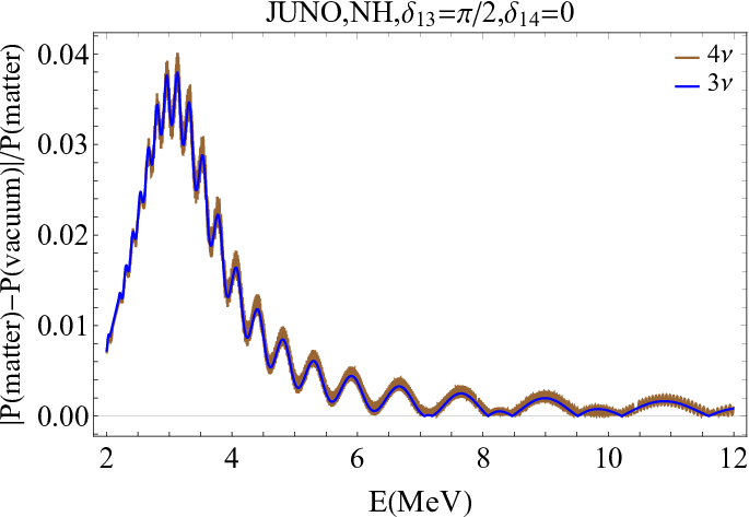
Regarding to matter effect, whether the oscillation probability will change with or without matter effect, both in purely 3 flavor active neutrinos case and in the framework of active plus sterile neutrino case, is what we are concerned. In Fig. 1 we take the relative difference for probability, from matter to vacuum, and plot it varying by energy. In order to discriminate the Dirac phases’ effect, we choose typic values of the two phases and make various combinations. In this analysis only normal hierarchy (NH) of neutrino mass situation is presented, while the inverted hierarchy (IH) case has similar behaviors, though not shown explicitly.
- 1)
Around the most promising range , the relative difference can reach , which could possibly be distinguished by JUNO detector.
- 2)
The sterile neutrino contribution does not affect probability curve dramatically, that is to say for short/medium baseline experiment, sterile neutrino effect is quite limited.
- 3)
The effect from Dirac phase seems bleak, no distinction can be reflected from different phase combinations.
Hence we may conclude that the short and medium baseline experiments are not sensitive to the matter effect of sterile neutrino, as well as the CP-violating Dirac phases.
4.2 Long baseline experiment
Neutrino beam produced from accelerators usually carries higher energy and can be detected in a long distance from source. In this part, we will take NOA experiment [31], with its baseline , as an example to illustrate the properties of long baseline experiments case.
Here we show the oscillation probability of appearance mode in long baseline accelerator neutrino experiment in Fig. 2, where the brown curves stands for oscillation in 3+1 scheme and blue curves correspond to SM case while solid (dashed) lines mean matter effect has (not) been contained. In the plot, we have chosen typical CP phase combination of () in NH case, and consider its variation in energy range . One can address the following points:
- 1)
The matter effect can not be negligible, on the contrary, it is important both in and case. At about range, the relative difference for probabilities can be as large as in whichever scenario. This difference could be around the maxima of oscillation probabilities.
- 2)
No matter propagating in vacuum or in matter, sterile neutrino gives nonnegligible contribution to oscillation probability. In each graph, the dashed lines have obvious deviation from their solid correspondence.
- 3)
The CP-violating Dirac phases also plays a non-ignorable role. By comparing Fig. 2a with Fig. 2c, one may see the oscillation probability has been affected. In the scenario of , one can see the blue lines are almost in the middle of corresponding brown lines. But the blue curves has a distinct deviation from the average lines of brown ones in the scenario of .
Therefore we may conclude that in the long baseline experiment, in the existence of sterile neutrino, the matter effect can not be ignored. The CP-violating Dirac phases in the mixing matrix may play an important role in sterile neutrino’s matter effect. A more comprehensive analysis to display the entanglement of the phases is necessary, and we will show it in other places.
 |
 |
| (a) | (b) |
 |
 |
| (c) | (d) |
5 Conclusion
In this work, we have derived exact formulas of oscillation probabilities with matter in medium and long baseline experiment in presence of an additional light sterile neutrino. In particular, the key quantities contributing to oscillation probability, and , are shown explicitly. Based on exact formulas, we perform a detailed study of the matter effect correction in medium and long baseline experiments. We found that in medium baseline experiment, like , the matter effect contribution is negligible even in presence of light sterile neutrino. But in the long baseline experiment, taking NOA as an example, the matter effect contribution plays a very important role especially when baseline grows.
Acknowledgements.
J. Ling acknowledges the support by National Key RD program of China under Grant No. 2018YFA0404103, NSFC (National Natural Science Foundation of China) under Grant No. 11775315 and young over-seas high-level talents introduction plan. F. Xu is supported partially by NSFC under Grant No. 11605076, as well as the FRFCU (Fundamental Research Funds for the Central Universities in China) under the Grant No. 21616309.Appendix A The parameterization of mixing matrix
In scenario, the full neutrino mixing is characterized by a matrix. To parameterize it, we need rotation angles and addtional Dirac phase angles.[32] The Majorana phase angles are closed here because it doesn’t involve in the oscillation process. The mixing matrix can be constructed by two-dimensional rotations
| (20) |
is a four dimensional rotation matrix, and in the sublocks its elements reads
| (21) |
with . The detailed matrix elements are
| (22) | ||||
Apparently if we close the angles related the forth neutrino, this lepton mixing matrix will reduce to PMNS matrix.
Appendix B Calculation of effective mass-square difference
In order to solve Eq.(7), we resort to solving a quartic equation in below, where its root is denoted as .
| (23) |
and the coefficients are defined as
| (24) |
with Levi-Civita symbol and . More auxiliary qualities are introduced to make the result more concise
| (25) |
With the above notations, we find solutions of
| (26) |
where . Notice that we don’t assume the a normal or inverted mass hierachy. Thus eq.(26) and the inequality above are hierachy independent. If neutrinos are in the inverted mass hierachy , we can simply set . If they are in the normal mass hierachy , the result is the eq.(10)
Appendix C Calculation of effective matrix
From Eq. (6), we may see the oscillation probability depends on some certain combinations of entries of , that is , where is not summed. In [25] some of the calculations has been done. The calculation of case can be confirmed, however, the result for seems wrong. Thus a reconsideration is required. In this section, we will complete this mission by an explicit calculation.
Since both and are unitary, one can subtract a diagonal matrix from Eq. (4) and Eq. (4), leading to
| (27) |
We can further write down
| (28) |
with .Similarly by taking the square and cube of Eq. (27), we can have equations corresponding to Eq. (28)
| (29) |
The square and cube on the right-handed side of (29) means The above equations can be written formally in a much more compact matrix, as
| (30) |
By solving linear equation Eq.(30) straightforwardly, we may get two classes of solutions shown below, denoted as and .
- 1)
The solution is
(31) with the auxiliary functions
(32) - 2)
Solution in this case is obtained as
(33) (34) in which we have especially introduced two important quantities,
(35) (36) In particular the second equation Eq. (34) is obtained by making use of the unitary property of .
References
- (1) P. Minkowski, Phys. Lett. 67B, 421 (1977). doi:10.1016/0370-2693(77)90435-X; T. Yanagida, Prog. Theor. Phys. 64, 1103 (1980). doi:10.1143/PTP.64.1103; R. N. Mohapatra and G. Senjanovic, Phys. Rev. Lett. 44, 912 (1980). doi:10.1103/PhysRevLett.44.912; J. Schechter and J. W. F. Valle, Phys. Rev. D 22, 2227 (1980). doi:10.1103/PhysRevD.22.2227.
- (2) M. Kohda, H. Sugiyama and K. Tsumura, Phys. Lett. B 718, 1436 (2013) doi:10.1016/j.physletb.2012.12.048 [arXiv:1210.5622 [hep-ph]].
- (3) W. F. Chang, S. C. Liou, C. F. Wong and F. Xu, JHEP 1610, 106 (2016) doi:10.1007/JHEP10(2016)106 [arXiv:1608.05511 [hep-ph]].
- (4) Y. Cai, J. Herrero-García, M. A. Schmidt, A. Vicente and R. R. Volkas, Front. in Phys. 5, 63 (2017) doi:10.3389/fphy.2017.00063 [arXiv:1706.08524 [hep-ph]].
- (5) Y. F. Li, Y. Wang and Z. z. Xing, Chin. Phys. C 40, no. 9, 091001 (2016) doi:10.1088/1674-1137/40/9/091001 [arXiv:1605.00900 [hep-ph]].
- (6) M. G. Aartsen et al. [IceCube and Fermi-LAT and MAGIC and AGILE and ASAS-SN and HAWC and H.E.S.S. and INTEGRAL and Kanata and Kiso and Kapteyn and Liverpool Telescope and Subaru and Swift NuSTAR and VERITAS and VLA/17B-403 Collaborations], Science 361, no. 6398, eaat1378 (2018) doi:10.1126/science.aat1378 [arXiv:1807.08816 [astro-ph.HE]]; M. G. Aartsen et al. [IceCube Collaboration], Science 361, no. 6398, 147 (2018) doi:10.1126/science.aat2890 [arXiv:1807.08794 [astro-ph.HE]].
- (7) A. Aguilar-Arevalo et al. [LSND Collaboration], Phys. Rev. D 64, 112007 (2001) doi:10.1103/PhysRevD.64.112007 [hep-ex/0104049].
- (8) A. A. Aguilar-Arevalo et al. [MiniBooNE Collaboration], Phys. Rev. Lett. 110, 161801 (2013) doi:10.1103/PhysRevLett.110.161801 [arXiv:1303.2588 [hep-ex]].
- (9) P. Adamson et al. [Daya Bay and MINOS Collaborations], Phys. Rev. Lett. 117, no. 15, 151801 (2016) Addendum: [Phys. Rev. Lett. 117, no. 20, 209901 (2016)] doi:10.1103/PhysRevLett.117.151801, 10.1103/PhysRevLett.117.209901 [arXiv:1607.01177 [hep-ex]].
- (10) M. G. Aartsen et al. [IceCube Collaboration], Phys. Rev. Lett. 117, no. 7, 071801 (2016) doi:10.1103/PhysRevLett.117.071801 [arXiv:1605.01990 [hep-ex]].
- (11) Y. J. Ko et al., Phys. Rev. Lett. 118, no. 12, 121802 (2017) doi:10.1103/PhysRevLett.118.121802 [arXiv:1610.05134 [hep-ex]].
- (12) S. Gariazzo, C. Giunti, M. Laveder and Y. F. Li, JHEP 1706, 135 (2017) doi:10.1007/JHEP06(2017)135 [arXiv:1703.00860 [hep-ph]].
- (13) F. Capozzi, C. Giunti, M. Laveder and A. Palazzo, Phys. Rev. D 95, no. 3, 033006 (2017) doi:10.1103/PhysRevD.95.033006 [arXiv:1612.07764 [hep-ph]].
- (14) N. Klop and A. Palazzo, Phys. Rev. D 91, no. 7, 073017 (2015) doi:10.1103/PhysRevD.91.073017 [arXiv:1412.7524 [hep-ph]].
- (15) S. Choubey, D. Dutta and D. Pramanik, Phys. Rev. D 96, no. 5, 056026 (2017) doi:10.1103/PhysRevD.96.056026 [arXiv:1704.07269 [hep-ph]].
- (16) S. Choubey, D. Dutta and D. Pramanik, arXiv:1711.07464 [hep-ph].
- (17) M. Ghosh, S. Gupta, Z. M. Matthews, P. Sharma and A. G. Williams, arXiv:1704.04771 [hep-ph].
- (18) D. Dutta, R. Gandhi, B. Kayser, M. Masud and S. Prakash, JHEP 1611, 122 (2016) doi:10.1007/JHEP11(2016)122 [arXiv:1607.02152 [hep-ph]].
- (19) F. Capozzi, C. Giunti, M. Laveder and A. Palazzo, Phys. Rev. D 95, no. 3, 033006 (2017) doi:10.1103/PhysRevD.95.033006 [arXiv:1612.07764 [hep-ph]].
- (20) S. K. Agarwalla, S. S. Chatterjee and A. Palazzo, JHEP 1804, 091 (2018) doi:10.1007/JHEP04(2018)091 [arXiv:1801.04855 [hep-ph]].
- (21) A. Chatla, S. Rudrabhatla and B. A. Bambah, arXiv:1804.02818 [hep-ph].
- (22) S. Gupta, Z. M. Matthews, P. Sharma and A. G. Williams, arXiv:1804.03361 [hep-ph].
- (23) M. Dentler, A. Hernández-Cabezudo, J. Kopp, P. Machado, M. Maltoni, I. Martinez-Soler and T. Schwetz, arXiv:1803.10661 [hep-ph].
- (24) B. Yue, W. Li, J. Ling, F. Xu, to appear soon.
- (25) H. Zhang, Mod. Phys. Lett. A 22, 1341 (2007) doi:10.1142/S0217732307022244 [hep-ph/0606040].
- (26) Y. Kamo, S. Yajima, Y. Higasida, S. I. Kubota, S. Tokuo and J. I. Ichihara, Eur. Phys. J. C 28, 211 (2003) doi:10.1140/epjc/s2003-01138-0 [hep-ph/0209097].
- (27) M. C. Gonzalez-Garcia, M. Maltoni and T. Schwetz, JHEP 1411, 052 (2014) doi:10.1007/JHEP11(2014)052 [arXiv:1409.5439 [hep-ph]].
- (28) S. Gariazzo, C. Giunti, M. Laveder and Y. F. Li, JHEP 1706, 135 (2017) doi:10.1007/JHEP06(2017)135 [arXiv:1703.00860 [hep-ph]].
- (29) I. Mocioiu and R. Shrock, Phys. Rev. D 62, 053017 (2000) doi:10.1103/PhysRevD.62.053017 [hep-ph/0002149].
- (30) F. An et al. [JUNO Collaboration], J. Phys. G 43, no. 3, 030401 (2016) doi:10.1088/0954-3899/43/3/030401 [arXiv:1507.05613 [physics.ins-det]].
- (31) D. S. Ayres et al. [NOvA Collaboration], doi:10.2172/935497
- (32) H. Fritzsch and Z. z. Xing, Prog. Part. Nucl. Phys. 45, 1 (2000) doi:10.1016/S0146-6410(00)00102-2 [hep-ph/9912358].