Self-Triggered Network Coordination over Noisy Communication Channels
Abstract
This paper investigates coordination problems over packet-based communication channels. We consider the scenario in which the communication between network nodes is corrupted by unknown-but-bounded noise. We introduce a novel coordination scheme, which ensures practical consensus in the noiseless case, while preserving bounds on the nodes disagreement in the noisy case. The proposed scheme does not require any global information about the network parameters and/or the operating environment (the noise characteristics). Moreover, network nodes can sample at independent rates and in an aperiodic manner. The analysis is substantiated by extensive numerical simulations.
I Introduction
Distributed coordination is one of the most active research areas in control engineering, with applications ranging from sensor fusion to optimization and control [1]. To achieve coordination, the network units (nodes) have to collect and process data from neighbouring nodes. In practice, a main issue is that the data transmission is often carried out through digital (i.e., packet-based) communication channels. Thus, coordination algorithms should take into account that the data exchange can only occur at finite rates and that the communication medium can introduce issues such as packet loss, transmission delay and noise.
The goal of this paper is to study coordination algorithms in the presence of communication noise, which is one of the major issues that arise in problems involving data exchange. We shall focus on consensus [1] algorithms since consensus is the prototypical problem in distributed coordination.
Literature review
Even if one neglects network-related issues such as finite transmission rate, dropouts and delay, developing noise-robust consensus algorithms is a very challenging task. The intuitive reason is that consensus algorithms usually rely on Laplacian dynamics. Since the Laplacian matrix is only marginally stable (has an eigenvalue at zero), communication noise can cause the state of the nodes to diverge. This means that even if consensus is achieved the consensus value need not be bounded, in which case convergence may become useless.
Most of the research works in this area assume that the noise has specific statistical properties, for example that it is white [2, 3], Brownian-like [4] or martingale [5, 6]. In contrast, only few research works have approached the problem where, due to uncertain channel characteristics, one can only regard noise as a bounded signal (unknown-but-bounded). Arguably, the lack of noise statistical properties makes it much more difficult to ensure state boundedness since one cannot rely on features such as as zero-mean or stationarity. In [7], the authors consider a Kalman-based coordination scheme, and show that consensus (the disagreement among the nodes) satisfies input-to-state stability properties, but no results are given regarding boundedness of the state trajectories. In [8], the authors study robust and integral robust consensus with respect to and norms of the noise function, but again the analysis only involves the disagreement variable and no results are given regarding state boundedness. This is also the case in [9] where the authors consider discrete consensus under bounded measurement noise, and in [10] where the authors propose discontinuous interaction rules to mitigate the effect of disturbances on the nodes disagreement. In the slightly different context of leader-following consensus, [11] considers the issue of sensor noise, but assumes that the noise is a smooth signal. While effective to account for sensor bias, this hypothesis is hardly met with communication noise. A framework closer to ours is in [12]. There, the authors propose a coordination scheme that guarantees approximate consensus along with boundedness of the state trajectories, but an upper bound on the magnitude of the noise is required to be known.
Summary of contributions
In this paper, we consider a novel coordination algorithm that can handle unknown-but-bounded noise without requiring the knowledge of a noise upper bound. In order to prevent state divergence, we propose a state-dependent coordination scheme where each node dynamically adjusts its update rule depending on the magnitude of its state. This approach can be regarded as a coarse dynamic quantization strategy, which updates the quantization based on the state of the nodes [13]. We show that this approach prevents state divergence and guarantees, in the noiseless case, a maximum consensus error for the worst case over the initial vector of states, which is reminiscent of normalized consensus metrics [14, 15]. As for the noisy case, we show that this approach guarantees that both disagreement and state variables scale nicely (linearly) with the noise magnitude.
From a technical point of view, our approach employs a self-triggered control scheme [16]. Each node uses a local clock to decide its update times. At each update time, the node polls its neighbors, collects the data and determines whether it is necessary to modify its controls along with its next update time. Similar to event-triggered control [17]-[18], self-triggered control [19]-[22] features the remarkable property that the communication among nodes occurs only at discrete time instants. Moreover, the nodes can sample independently and aperiodically. Thus, the proposed approach is appealing also from the perspective of finding coordination algorithms that are practically implementable (as we will see, including the case where the data exchange encounters delays).
The proposed self-triggered algorithm shares similarities with several pairwise gossip or multi-gossip approaches with randomized [23] and deterministic [24] protocols. There is however a major difference, namely that while for gossiping algorithms the inter-node interaction times occur at multiples of discrete time-steps, in self-triggered consensus algorithms the update instants are established on the basis of current node measurements and can take any value on the continuous-time axis. Moreover, to the best of our knowledge, gossiping has not been considered in connection with unknown-but-bounded noise, even in the recent literature [25]-[26].
A preliminary version of the manuscript appeared in [27]. Compared with the latter, this paper provides complete proofs of all the results, a thorough discussion of the proposed method and extensive numerical results. Furthermore a new section considering the presence of delays in the communication channel is considered.
The remainder of the paper is as follows. In Section II, we introduce the framework of interest and outline the main paper results. The proposed coordination scheme is introduced in Section III, and the main results are discussed throughout Sections IV and V. Section VI further discusses properties of the proposed coordination scheme. Numerical examples are illustrated in Section VII. Section VIII ends the paper with concluding remarks. In the Appendix, the main results of the paper are extended to include communication delays.
I-A Notation
We assume to have a set of nodes and an undirected connected graph , where is the set of edges (links). We denote by the Laplacian matrix of , which is a symmetric matrix. For each node , we denote by the set of its neighbors and by its degree, that is, the cardinality of . Given scalar-valued variables , we define . Given a vector , denotes its Euclidean norm and its infinity norm. Given a signal mapping to , we define and say that is bounded if is finite.
II Framework and Outline of the Main Results
II-A Network dynamics
We consider a network of dynamical systems that are interconnected over an undirected graph . Each node is described by
where ; is the state; is the control input, and is the output where is a bounded signal, which models communication noise. Note that this model implies that all the neighbors of node will receive the same corrupted information. As it will become clear in the sequel, it is possible to replace the second of (II-A) with , where and , so that each neighbor of node receives a different corrupted information. We will not pursue this model in order to keep the notation as streamlined as possible.
According to the usual notion of consensus [1], the network nodes should converge, asymptotically or in a finite time, to an equilibrium point where all the nodes have the same value lying somewhere between the minimum and maximum of their initial values. In the presence of noise, however, convergence to an exact common value is in general impossible to achieve. As outlined hereafter, the main contribution of this paper is a new coordination scheme that ensures practical (approximate) consensus, namely convergence to a set whose radius depends on the noise amplitude.
II-B Outline of the main results
One way to define practical consensus is via the normalized error between the nodes. We consider a coordination scheme that, in the noiseless case, guarantees that all the network nodes remain between the minimum and the maximum of their initial values, and converge in a finite time to a point belonging to the set
| (4) |
where is a design parameter, and . In words, when the coordination scheme guarantees that, in a finite time, each node reaches a local average that satisfies
| (5) |
The parameter determines the desired accuracy level for the consensus final value, which is normalized to the magnitude of the initial data. In this way, a maximum error is guaranteed for the worst case over the initial vector of measurements. If instead then the tolerance reduces to . We will further comment on this point in Section VI.
As for the noisy case, the coordination scheme guarantees that the error scales nicely with respect to the noise magnitude. Specifically, let
| (6) |
where denotes the maximum among the nodes degrees. The scheme guarantees that, in a finite time, the network state enters the set
| (7) |
and remains there forever with convergence in the event that goes to zero. Moreover, the state remains confined in a set whose radius depends on and .
From an implementation point of view, the proposed scheme enjoys the following features:
- (i)
No knowledge of is required.
- (ii)
No knowledge of is required.
- (iii)
The control action is fully distributed.
- (iv)
The communication between network nodes occurs only at discrete time instants. Moreover, the nodes can sample independently and in an aperiodic manner.
These features indicate the implementation does not require any global information about the network parameters and/or the operating environment (the noise). The last feature renders the proposed scheme applicable when coordination is through packet-based communication networks.
The main derivations will be carried out assuming that there are no communication delays, which are dealt with in the Appendix section. The analysis shows that, in practice, delays have the same effect as an additional noise source. For this reason, also numerical simulations will be restricted to the delay-free case.
III Self-triggered Coordination with Adaptive Consensus Thresholds
III-A Adaptive consensus thresholds
As discussed in the previous section, we aim at considering a normalized error between network nodes. To this end, each node has a local variable
that specifies the threshold used to assess whether or not consensus is achieved. In contrast with previous self-triggered schemes [16, 28], this threshold is adaptive as it scales dynamically with the state magnitude. It is exactly this feature that ensures robustness against noise.
Notice that is used by node to construct the threshold , which amounts to assuming that each node has access to its own state without noise. This assumption can be relaxed and all the results continue to hold with the difference that the state bound (2) and the consensus set radius ( in equation (6)) will be enlarged. We neglect the details for this situation since it does not affect the general idea of the paper.
III-B Control action and triggering times
For each , let with be the sequence of time instants at which node collects data from its neighbors. At these time instants, the node updates its control action and determines when the next update will be triggered.
For each , let
| (11) |
denote the local noisy average.
The control action makes use of a quantized function, The control signals take values in the set , and the specific quantizer of choice is , , which is given by
| (12) |
The control action is given by
| (13) |
for .
The triggering times are given by , where
Note that by construction the inter-sampling times are bounded away from zero. This guarantees the existence of a unique Carathèodory solution for the state trajectories.
Remark 1
In the noise-free case, the control law (13) is an approximation of the pure (non-quantized) sign function which yields “max-min” consensus [29], that is convergence to the centre of the interval containing the nodes initial values. Specifically, in the noise-free case, the scheme reduces to the one in [29] when and the flow of information among nodes is continuous. We refer the reader to Sections VII-B for further discussions on this point.
Remark 2
Although the paper focuses on networks of dynamical systems of the form (II-A), it is not hard to tackle synchronization problems involving linear dynamics as in [30], since synchronization can be reduced to a consensus problem by means of suitable coordinate transformations. For the noise-free case self-triggered algorithms for the synchronization of linear systems have been studied in [31], and for the noise-free case with packet dropouts in [32]. These algorithms can be modified in the spirit of (III-A)-(III-B) for the case of noisy measurements and the analysis carried out in the rest of the paper can be extended to the synchronization problem of linear systems.
IV Noiseless Case
We start by investigating the properties of this coordination scheme in the absence of communication noise. For ease of notation, we let
| (17) |
denote the noiseless average. Note that in the noiseless case for every .
Let
| (18) |
We have the following result.
Theorem 1
Consider a network of dynamical systems as in (II-A) with , which are interconnected over an undirected connected graph . Let each local control input be generated in accordance with (III-A)-(III-B). Then, for every initial condition, the state converges in a finite time to a point belonging to the set in (4). Moreover, and for every .
Proof. We start with showing the last property. We only show that for every since the other case is analogous. We prove the claim by contradiction. Suppose there exists a time such that and , with being the index of the node exceeding for the first time (clearly, more than one node could exceed at the same time but this does not affect the analysis). Note that cannot be a switching time for node . In fact, if this were true, then we would have , which would require , which is not possible because for all , by definition of and . Thus, we focus on the case where is not a switching time.
Let be the last sampling instant smaller than , which implies for all . Notice that is well defined even if occurs during the first inter-sampling interval of node because for all . Since for all , it holds that
| (19) |
Evaluating the last identity at , we get
| (20) |
Observe now that in order for to grow we must also have . This requires . In fact, if then node could not grow as for all . By (III-B), we have
| (21) | |||||
where the inequality comes again from the fact that for all . The proof follows recalling the inequality (20). In fact, this implies
| (22) |
which is not possible since .
We now focus on the property of convergence. Consider the Lyapunov function
| (23) |
where is the Laplacian matrix related to the graph . By letting , the evolution of along the solutions to (II-A) satisfies
| (24) | |||||
where the last equality follows from the definition of the quantized sign function. Observe now that if then
| (25) | |||||
for all . This implies that preserves the sign during continuous flow. Similarly, if then
| (26) | |||||
Hence,
| (27) | |||||
This leads to
| (28) | |||||
since for all . Thus, there exists a finite time such that each node satisfies for every such that , otherwise would take on negative values. This shows that all the controls eventually become zero, which implies that for all . Hence, we also have for all and for all . Since the network state remains within the initial envelope, we have for all and for all , which yields the desired result.
V Noisy Case
In this section, we study convergence and boundedness properties of the proposed scheme in the presence of noise. We first show that the proposed coordination method ensures boundedness of the state trajectories.
V-A Boundedness of the state trajectories
Let
| (29) |
We have the following result.
Theorem 2
Proof. We will only prove the result regarding since the other can be proved in an analogous manner. Notice that for all and all , where we defined
| (36) |
Clearly, we have
| (37) |
for all and all .
Case 1: . We show that there is no node that can exceed . Suppose that there exists a time such that and , with the index of the node exceeding for the first time (clearly, more than one node could exceed at the same time but this does not affect the analysis). In contrast with the proof of Theorem 1, here may potentially be a switching time, since it could happen that even though for all due to the presence of the noise . The case in which is a switching instant falls into the case studied in the next paragraph.
Let be the last sampling instant not greater than , which implies for all . Notice that is well defined even if occurs in the first inter-sampling interval of node since for all . We have two sub-cases.
Sub-case 1: . The condition for to grow is
| (38) |
Since for all , we have
| (39) | |||||
By combining (37) and (39), in order for to grow we must necessarily have
| (40) |
This leads to a contradiction. In fact, if then . Moreover, . Hence, we must necessarily have
| (41) |
which implies , thus leading to a contradiction. If instead then and we must have
| (42) |
This leads again to a contradiction since, by hypothesis, we must have and . This would imply .
Sub-case 2: . By construction, can grow at most up to
| (43) |
where the inequality follows since for all . Since we conclude that can grow at most up to
| (44) |
which leads to a contradiction.
Case 2. . The proof of this case is exactly same as for the previous case with replaced by .
V-B Consensus properties under low-magnitude noise
We start with a simple result which shows that convergence is preserved under noise whenever is sufficiently small compared to . Moreover, the state remains within the initial envelope like in the noiseless case.
Theorem 3
Consider a network of dynamical systems as in (II-A), which are interconnected over an undirected connected graph . Let each local control input be generated in accordance with (III-A)-(III-B). Suppose that . Then, for every initial condition, the state converges in a finite time to a point belonging to the set in (7). Moreover, and for all .
Proof. We first show the last property. This can be done following the same steps as in the noiseless case. Again, we only show that for all . Suppose that there exists a time such that and , with the index of the first node exceeding (clearly, more than one node could exceed at the same time but this does not affect the analysis). Let be the last sampling instant not greater than , which implies for all . Notice that is well defined even if occurs during the first inter-sampling interval of node because for all . Clearly, we must necessarily have . Moreover,
| (45) |
for all .
By (III-B), we have
| (46) | |||||
where the inequality follows from the fact that for all . By hypothesis, is the last sampling instant not greater than . Hence, since the control input is constant over and because must exceed we must have . Hence,
| (47) |
This inequality is possible only when
| (48) |
However, this implies
| (49) | |||||
where the last inequality follows since by hypothesis. This implies that , thus leading to a contradiction.
We now focus on convergence. Let be defined as in (23), and consider the evolution of along the solutions to (II-A). By letting , we have
| (50) | |||||
where the last equality follows from the definition of the quantized sign function. Observe now that if then . Moreover,
| (51) | |||||
for all . Similarly, if then , and
| (52) | |||||
This leads to
| (53) |
for all . Since ,
| (54) |
for some , since all the quantities involved are constant. Hence, there exists a finite time after which each node satisfies for every such that , otherwise would take on negative values. Since remains within the initial envelope then for all . Thus for every . This shows that all the controls eventually become zero not later than , which implies that and for all . Moreover, since remains within the initial envelope we also have for all . Taking any we then have
| (55) | |||||
The proof is concluded by noting that the right side of (55) is upper bounded by .
V-C Consensus properties under general noise
In general, condition need not be satisfied if is unknown. Even if is known, enforcing this condition might lead to large errors between network nodes. To this end, we study the properties of the proposed approach for the general case of noise which are unknown but bounded. We have the following result.
Theorem 4
Consider a network of dynamical systems as in (II-A), which are interconnected over an undirected connected graph . Let each local control input be generated in accordance with (III-A)-(III-B). Then, for every initial condition, the network state enters in a finite time the set in (7) and remains there forever. Moreover, converges in a finite time to a point belonging to the set in (7) when the noise converge to zero.
We prove two technical results which are instrumental for the proof of Theorem 4.
The first result relates and .
Lemma 1
Consider the same assumptions and conditions as in Theorem 4. For any , it holds that
| (56) |
for every .
Proof. By Theorem 2, we have
| (57) |
Hence,
| (58) | |||||
where the last equality holds by the definitions (6) and (29) of and respectively.
The second result shows that the average preserves the sign as long as its absolute value remains large enough compared with the radius .
Lemma 2
Consider the same assumptions and conditions as in Theorem 4. Consider any index and any . If for then
| (59) |
Proof. Assume without loss of generality that , the other case being analogous. From Lemma 1, we have
| (60) | |||||
Hence, . Moreover,
| (61) | |||||
for all .
We then conclude that . Thus preserves its sign.
We can now proceed with the proof of Theorem 4.
Proof of Theorem 4. We only show the result for the case since the other case can be derived from Theorem 3. To begin with, we introduce three sets into which we partition the set of switching times of each node . For each , let
Clearly, for every .
Pick any , and assume by contradiction that there exists a time such that for all . In view of Lemma 1, is never zero from on since the condition above yields . Moreover, by Lemma 2, for every . Hence, either for all or for all . This would imply that diverges, violating the state boundedness property of Theorem 2.
By the foregoing arguments, there exists a time instant such that . This implies that , or, equivalently, that . Thus it remains to show that transitions from and to are not possible. We analyze the two cases separately.
Case 1: . In this case, . Suppose that , the other case being analogous. Then,
| (66) |
for all where the first inequality follows since while the second inequality follows because by hypothesis. In addition, condition implies . Thus,
| (67) | |||||
for all . Thus which implies that .
Case 2: . In this case we have for all and . Hence,
| (68) | |||||
for all , where the third inequality follows from and the fourth one follows from Lemma 1. Hence, .
Hence, we conclude that for all . Moreover, the previous arguments show that for all , for all , which guarantees that remains forever inside . Finally, if converges to zero then there exists a finite instant such that , and the convergence result follows along the same lines as in Theorem 3.
VI Adaptive Thresholds, Sign Function and Node-to-node Error
In this section, we further comment on the considered notion of consensus and discuss a number of properties ensured by the proposed coordination scheme.
VI-A Adaptive thresholds and sign function
The main problem when dealing with communication noise is that the Laplacian graph matrix has an eigenvalue in zero. This may cause the state to drift when the noise has non-zero mean. In this paper, drifting is prevented by resorting to local adaptive thresholds
These adaptive thresholds scale with the magnitude of the data and this feature is essential to guarantee that any drifting will eventually stop. Specifically, recall that the local control action is given by
| (72) |
where
| (73) |
Suppose that starts drifting, for example growing (). Since then cannot grow, so that must remain bounded. Hence, adapting the threshold of the function to the magnitude of eventually forces to become larger than . We will exemplify this feature in Section VII-A. In contrast, a pure constant need not counteract the drifting of since may persistently remain larger than .
Another interesting feature of the proposed scheme lies in the use of the function. When the level of disagreement is large compared with the noise magnitude, for example during the initial phase of coordination, then . In this situation, the function ensures that the control action will be the same as in the noiseless case. In other terms, the noise will affect coordination only when nodes are sufficiently close to consensus. Also this feature will be exemplified in Section VII-A.
The function does also permit to save communication resources, which is one of the main issues when coordination is carried out through packet-based networks. Recall that in the proposed scheme the inter-transmission times are defined as
As noted before, when is large compared with the noise magnitude, then and the control action behaves as in the noiseless case. In the proposed scheme, condition is implemented as . In particular, when then increases with with the idea that large values of correspond to a situation where the disagreement is large so that there is no need for very frequent control variations. The situation is different when . In this case, it may happen that is significantly different from . Moreover, also implies that the level of disagreement is small compared with the data magnitude. Thus, if then is decreased to with the idea that control variations should be made more frequent so as to counteract the effect of noise and maintain a small level of disagreement. Clearly, in this situation may become small if is chosen small, and the latter is desired to ensure a small level of disagreement. As discussed in the next subsection, there is actually no need to pick very small in order to secure a small level of disagreement, which means that communications need not be frequent even when the nodes are within the consensus region.
VI-B Node-to-node error
The proposed coordination scheme guarantees that, in the noiseless case, all the nodes remain between the minimum and the maximum of their initial values, and converge in a finite time to a point belonging to the set
| (77) |
where is a design parameter, and . As noted, when the coordination scheme guarantees that, in a finite time,
| (78) |
The parameter determines the desired accuracy level for the consensus final value, which is normalized to the magnitude of the initial data. In this way, a maximum error is guaranteed for the worst case over the initial vector of measurements. If instead then the tolerance becomes . The parameter plays a crucial role for consensus. On one side, it is desirable to choose so as to guarantee a small level of disagreement. On the other hand, a very small value of can render the coordination scheme very sensitive to noise. Moreover, as noted before, small values of can induce large communication rates since determines the smallest inter-transmission time of each node. It is the term that somehow makes this tradeoff less critical.
At first glance, it seems indeed more natural to search for coordination schemes that guarantee
| (79) |
or node-to-node error. In fact, the latter guarantees that the disagreement is small for every pair of nodes (not necessarily connected), while (78) only ensures that the disagreement is small locally (for its neighbourhood). Actually, in many cases of practical interest it turns out that a bound on the local averages implies a bound on the node-to-node error which is strictly smaller than . In this situation, working with (78) is advantageous compared with (79) since this guarantees a small node-to-node error without requiring to choose too small. In turn, this moderates the noise sensitivity and the number of communications. As discussed next, this situation happens when the network connectivity is sufficiently large. We make this argument precise.
Consider the same setting as in Theorem 4, and let denote the time after which the network state remains confined in . Pick any fixed time instant and let and denote the network nodes taking on maximum and minimum value, respectively. The indices and may change with time but we consider a fixed . Let with (the case is not interesting because the network would be at perfect consensus). By Theorem 4, for all . We now relate and . First notice that
| (80) | |||||
where we omitted the time argument for brevity. Decompose . Since for all , we obtain
| (81) |
where
Moreover,
| (86) |
where
In fact, for every set because and is the node that takes on the minimum value in the network. In addition, if we then have , which implies . Since , we get
| (90) | |||||
which implies
| (91) |
assuming .
The quantity represents the number of neighbors that are common to and . Since it is then sufficient that in order to guarantee that . Even more, may become significantly smaller than for large values of . Consider for example the case of complete graphs. In this case, , and . Hence,
| (92) |
Since we always have . Moreover, recalling that , one sees that in the noiseless case actually decreases with whenever the initial conditions do not depend on the network size, and remains bounded irrespective of with a maximum noise amplification factor equal to .
The considerations made above apply in general since (91) does not depend on the network topology. In fact, (91) suggests that working with (78) can be advantageous compared with (79) whenever the network connectivity is sufficiently large. We will further substantiate this analysis in Section VII-B through numerical simulations.


VII Numerical Examples
In this section, we illustrate the proposed consensus scheme through a number of numerical examples.
VII-A Small graph
This example is used to illustrate the main results of this paper in an easy-to-follow manner. We consider a simple cycle graph with nodes, which implies . Moreover, we let . The initial value of each network node is taken as a random number within .
Low-magnitude noise. To begin with, we assume that the noise are generated randomly within , which implies . The simulation results are reported in Figure 1, which shows trajectory of the states , absolute values of local averages , and local controls for nodes , and . One sees that the conditions of Theorem 3 are verified in the sense that the network state eventually converges and the local controls become zero, which occurs after . In Figure 1(b), the blue dot-dash line represents the bound on dictated by Theorem 3. In this example, . Moreover, by Theorem 2 the state evolution remains confined in the initial envelope since .
General case: Zero mean noise. We next assume that the noise for node is given by
| (93) |
where is generated randomly within and . This implies so that . Simulation results are shown in Figure 2, from which one sees that the state enters the set around and remains there forever, while the local controls continue to switch. This is in agreement with Theorem 4, as well as the discussion in Remark 3.
General case: Sign-preserving noise. We finally assume that the noise are generated randomly within , which implies again . Since the Laplacian has an eigenvalue in zero, constant or sign-preserving noise represent a critical situation since they can induce drifting phenomena. This phenomenon is shown in Figure 3. One sees that the proposed coordination scheme prevents the state from growing unbounded. In particular, in agreement with Theorem 2 the state remains within the interval with (red dot-dash line in Figure 3(a)). In agreement with Theorem 4, the network state enters in a finite time the set and remains there forever. Figure 3(b) shows that the theoretical bound (blue dot-dash line) is conservative as each local average eventually becomes very small. From Figure 3(c) one sees that the local controls do not switch as fast as in the beginning. This is expected since, as state increases, also the threshold increases. This makes the noisy average likely to be confined within , causing the control switches to be more and more sporadic.


VII-B Erdös-Rényi and random geometric graphs
In this section, we illustrate the proposed scheme for graphs of a larger size and exemplify some of the considerations made in Section VI-B, focusing on two well-known graphs: Erdös-Rényi (ER) and random geometric (RG) graphs [33]. The former is obtained from the -dimensional complete graph by retaining each edge with probability (independently). The latter is obtained by considering a random uniform deployment of points in a -dimensional Euclidian space. Denoting by the position of node , a link between nodes and exists if and only if where denotes the communication range, which is assumed identical for every node.
For both the graphs we consider Monte Carlo simulations. Specifically, we consider trials. For each trial, we generate an ER (RG) graph of nodes. Graphs which are not connected are not taken into account. For the ER graph we consider a link probability , while for the RG graph we consider a random deployment over a region of with nodes communication range . For each trial, the nodes initial values are taken randomly within , and the noise is taken as a random number within . The sensitivity parameter is for all the trials.
Let be the sequence of time instants at which one of the nodes samples, i.e. for some and . Given a simulation horizon , this sequence will range from up to where is the largest integer such that . The asymptotic behavior of the nodes is defined as the behavior of the nodes over the time interval , where is a positive integer that is selected so as to satisfy and . The reason for this choice is twofold: (i) since the network nodes need not converge, it makes little sense to consider only the value of the nodes at the final step . In this respect, makes it possible to evaluate the network behavior for a sufficiently large number of samples; (ii) we aim at evaluating the network limiting behavior, i.e. after the transient has vanished. Hence, guarantees that initial samples are not taken into account. In the simulations, for each trial, we consider, and . We consider three performance indices:
- 1.
Asymptotic maximum local average. This index is given by
Basically, for each of the trials, we compute the average of the largest value of the local averages over the time interval . Then, these values are averaged over the number of trials.
- 2.
Asymptotic maximum node-to-node distance. This index is given by
Here, for each trial, we compute the average of the largest value of the node-to-node distances over the interval . As before, these values are then averaged over the number of trials.
- 3.
Asymptotic maximum distance from the expected convergence point. This index is given by
where
(94) This performance index is similar to , with the exception that the nodes values are compared to the midpoint of the maximum and minimum initial values of the nodes. This is because our algorithm can be viewed as an approximation of the pure -consensus, which is known to converge to [29].
The results are reported in Figure 4. Figure 4(a) confirms the bound obtained in Theorem 4, showing that the local averages scale nicely with (cf. (6)). More interesting is the result in Figure 4(b) which shows that the node-to-node error decreases as the number of nodes increases. This can be explained by observing that for both the graphs the expected number of common neighbors increases with , which causes in (91) to decrease in agreement with the comments made in Section VI-B. In particular, for the ER graph the expected number of common neighbors between two network nodes is given by , while for the RG graph the probability that two nodes are connected is given by where is the area of the deployment region, and the expected number of common neighbors between two connected nodes is approximately [34]. This can explain why is smaller for the ER graph. Figure 4(c) finally shows that the distance from the expected convergence point is indeed small and decreases with . The latter property can be explained by noting that large values of decrease the effect of (cf. Section VI-B), which causes the quantized sign function to better approximate the pure function.
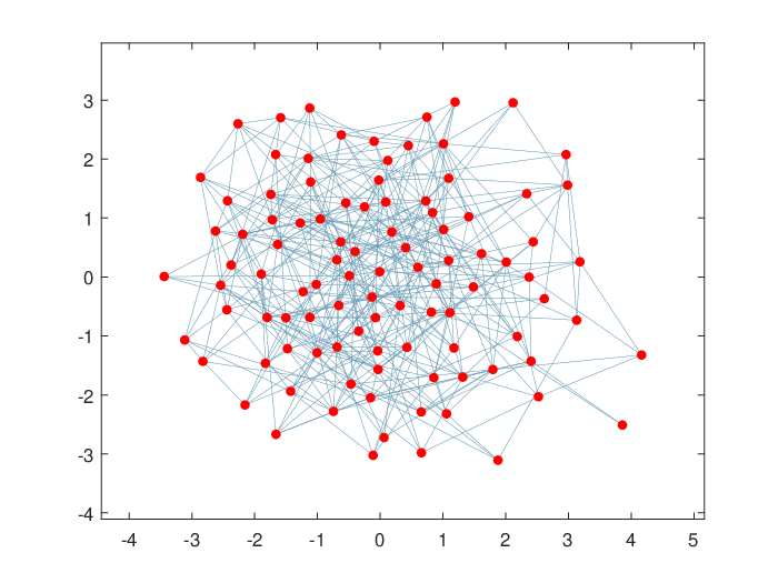
We report in Figures 5 and 6 the results of one of the trials for the ER graph. In this trial, we obtain which leads to and . The large theoretical bounds are due to the large value of . In practice, as show in Figure 6, the regulation performance is very high. In fact, the absolute value of the noiseless averages is eventually upper bounded by , which is much smaller than the theoretical bound given by . We omit the simulation results of one trial for the RG graph since the figures are similar to the ones for the ER graph.


VIII Conclusions
In this paper, we proposed a novel self-triggered network coordination scheme that can handle unknown-but-bounded noise affecting the network communication. The proposed coordination scheme employs a dynamic, state-dependent, triggering policy and ternary controllers. It has been shown that the scheme can achieve finite-time practical consensus in both noiseless and noisy cases. In the latter situation, the node disagreement value scales nicely with the magnitude of the noise. An interesting feature of the proposed scheme is that the implementation does not require any global information about the network parameters and/or the operating environment. Moreover, the communication between nodes occurs only at discrete time instants, and nodes can sample independently and in an aperiodic manner. The last feature renders the proposed scheme applicable when coordination is through packet-based communication networks.
An interesting outcome of this work is that the proposed scheme can guarantee a small node-to-node error without requiring to choose the consensus threshold too small. In turn, this can be beneficial for moderating the noise sensitivity as well as the number of communications. Investigating this point in more details certainly represents an interesting venue for future research.
Communication Delays
In this section, we briefly discuss how transmission delays can be taken into account. Some of the derivations follow closely the delay-free analysis of Section III-B so that we will discuss in detail only the points where substantial differences appear.
For each , let with be the sequence of time instants at which node starts collecting data from its neighbors. Given a neighbor , node will receive information from at a certain time , where represents the total delay in the communication between and . In general, can be time-varying (dependence on ) as well as link-dependent (dependence on and ). At , the information received by node is given by for some , which represents the time at which transmits its value. At time
| (95) |
node will then have all the information needed to update its control action. Accordingly, will define the sequence of control updates.
The control action is given by
where
| (100) |
The rationale is the following. Before time , node has no information from the whole neighboring set so that its control action is set to zero. On the other hand, is nothing but the natural generalization of the control action considered in the delay-free case, where the additional superscript indicates the presence of delays.
The triggering instants are now given by , where
which is also the natural generalization of the triggering rule considered in the delay-free case. As before, by construction the inter-sampling times are bounded away from zero. Notice that by construction with equality holding if and only if delays are zero, and .
Approaching the analysis directly with respect to is not simple because contains data which are collected at different time instants. Nonetheless, one can simplify the analysis by exploiting the special structure of the control law. Rewrite
| (104) | |||||
where
| (105) |
Since the control action does always belong to and since , we are guaranteed that , where
| (106) |
represents the maximum delay that can occur over a network communication link. It follows that
| (107) | |||||
This suggests that the analysis for the case of delays can be approached as in the delay-free case by considering a different, possibly larger, noise contribution.
The first result is concerned with boundedness of the state trajectories, and is a straightforward variation of Theorem 2.
Let
| (108) |
Theorem 5
Consider a network of dynamical systems as in (II-A), which are interconnected over an undirected connected graph . Let each local control input be generated in accordance with (Communication Delays)-(Communication Delays). Then, for every initial condition, the state satisfies
and
for every .
Proof. The proof follows exactly the same steps as the proof of Theorem 2 using condition for Sub-case 1 and condition for Sub-case 2.
The counterpart of Theorem 4 is slightly more involved but it essentially follows the same reasoning of Section V-C.
Let
| (115) |
Theorem 6
Consider a network of dynamical systems as in (II-A), which are interconnected over an undirected connected graph . Let each local control input be generated in accordance with (Communication Delays)-(Communication Delays). Assume that noise and delays are such that . Then, for every initial condition, the network state enters in a finite time the set
| (116) |
and remains there forever.
The proof of Theorem 6 hinges upon two technical results, which extend Lemma 1 and 2 to the presence of delays.
Lemma 3
Consider the same assumptions and conditions as in Theorem 6. For any , it holds that
| (117) |
for every .
Proof. By Theorem 5, we have
| (118) |
Hence,
| (119) | |||||
where the last inequality holds by the definitions (115) and (108) of and respectively.
Lemma 4
Consider the same assumptions and conditions as in Theorem 6. Consider any index and any . If for then
| (120) |
Proof. Assume without loss of generality that , the other case being analogous. From Lemma 3, we have
| (121) | |||||
Hence, . Moreover,
| (122) | |||||
for all . The first inequality comes from the fact that the control inputs always belong to . Thus, over the time interval , the value of can decrease at most with slope . The second inequality follows because .
We then conclude that . Thus preserves its sign.
We can now proceed with the proof of Theorem 6.
Proof of Theorem 6. Like in the proof of Theorem 4, we introduce three sets into which we partition the set of switching times of each node . For each , let
Clearly, for every .
Pick any , and assume by contradiction that there exists a time such that for all . In view of Lemma 3, is never zero from on since the condition above yields . Moreover, by Lemma 4, for every . Hence, either for all or for all . This would imply that diverges, violating the state boundedness property of Theorem 5.
By the foregoing arguments, there exists a time instant such that . This implies that , or, equivalently, that . Thus it remains to show that transitions from and to are not possible. We analyze the two cases separately.
Case 1: . In this case, . Suppose that , the other case being analogous. Then,
| (127) |
for all , where the first inequality follows since and the second because by hypothesis. Moreover, implies so that . Hence,
| (128) | |||||
for all . Hence, which implies that .
Case 2: . In this case we have for all . Since then so that . Moreover, . Hence,
| (129) | |||||
for all , where the third inequality follows from and the fourth one follows from Lemma 3. Hence, .
Hence, we conclude that for all . Moreover, the previous arguments show that for all , for all , which guarantees that remains forever inside .
Following the same steps as in Section V-B, it is an easy matter to see that if then the state converges in a finite time to a point belonging to the set , which parallels the result in Theorem 3.
We close this section by pointing out that less conservative bounds can be obtained under the additional hypothesis that the messages are time-stamp synchronized, in which case one can assume that if node sends a request to node at time then is capable of providing node with the value . This scenario has been studied in [16].
References
- [1] Y. Cao, W. Yu, W. Ren, and G. Chen, “An overview of recent progress in the study of distributed multi-agent coordination,” IEEE Transactions on Industrial informatics, vol. 9, no. 1, pp. 427–438, 2013.
- [2] T. Li and J.-F. Zhang, “Mean square average-consensus under measurement noises and fixed topologies: Necessary and sufficient conditions,” Automatica, vol. 45, no. 8, pp. 1929–1936, 2009.
- [3] L. Cheng, Z.-G. Hou, M. Tan, and X. Wang, “Necessary and sufficient conditions for consensus of double-integrator multi-agent systems with measurement noises,” IEEE Transactions on Automatic Control, vol. 56, no. 8, pp. 1958–1963, 2011.
- [4] T. Li, F. Wu, and J.-F. Zhang, “Multi-agent consensus with relative-state-dependent measurement noises,” IEEE Transactions on Automatic Control, vol. 59, no. 9, pp. 2463–2468, 2014.
- [5] T. Li and J.-F. Zhang, “Consensus conditions of multi-agent systems with time-varying topologies and stochastic communication noises,” IEEE Transactions on Automatic Control, vol. 55, no. 9, pp. 2043–2057, 2010.
- [6] M. Huang, S. Dey, G. N. Nair, and J. H. Manton, “Stochastic consensus over noisy networks with markovian and arbitrary switches,” Automatica, vol. 46, no. 10, pp. 1571–1583, 2010.
- [7] D. B. Kingston, W. Ren, and R. W. Beard, “Consensus algorithms are input-to-state stable,” in American Control Conference, 2005. Proceedings of the 2005. IEEE, 2005, pp. 1686–1690.
- [8] G. Shi and K. H. Johansson, “Robust consensus for continuous-time multiagent dynamics,” SIAM Journal on Control and Optimization, vol. 51, no. 5, pp. 3673–3691, 2013.
- [9] A. Garulli and A. Giannitrapani, “Analysis of consensus protocols with bounded measurement errors,” Systems & Control Letters, vol. 60, no. 1, pp. 44–52, 2011.
- [10] M. Franceschelli, A. Giua, A. Pisano, and E. Usai, “Finite-time consensus for switching network topologies with disturbances,” Nonlinear Analysis: Hybrid Systems, vol. 10, pp. 83–93, 2013.
- [11] E. Arabi, T. Yucelen, and W. M. Haddad, “Mitigating the effects of sensor uncertainties in networked multi-agent systems,” Journal of Dynamic Systems, Measurement, and Control, vol. 139, no. 4, p. 041003, 2017.
- [12] D. Bauso, L. Giarré, and R. Pesenti, “Consensus for networks with unknown but bounded disturbances,” SIAM Journal on Control and Optimization, vol. 48, no. 3, pp. 1756–1770, 2009.
- [13] R. Carli, F. Bullo, and S. Zampieri, “Quantized average consensus via dynamic coding/decoding schemes,” International Journal of Robust and Nonlinear Control, vol. 20, no. 2, pp. 156–175, 2010.
- [14] S. Boyd, A. Ghosh, B. Prabhakar, and D. Shah, “Randomized gossip algorithms,” IEEE/ACM Transactions on Networking (TON), vol. 14, no. SI, pp. 2508–2530, 2006.
- [15] A. G. Dimakis, S. Kar, J. M. Moura, M. G. Rabbat, and A. Scaglione, “Gossip algorithms for distributed signal processing,” Proceedings of the IEEE, vol. 98, no. 11, pp. 1847–1864, 2010.
- [16] C. De Persis and P. Frasca, “Robust self-triggered coordination with ternary controllers,” IEEE Transactions on Automatic Control, vol. 58, no. 12, pp. 3024–3038, 2013.
- [17] W. Heemels, K. H. Johansson, and P. Tabuada, “An introduction to event-triggered and self-triggered control,” in Decision and Control (CDC), 2012 IEEE 51st Annual Conference on. IEEE, 2012, pp. 3270–3285.
- [18] C. Nowzari, J. Cortes, and G. J. Pappas, “Event-triggered communication and control for multi-agent average consensus,” Cooperative Control of Multi-Agent Systems: Theory and Applications, p. 177, 2017.
- [19] A. Anta and P. Tabuada, “To sample or not to sample: Self-triggered control for nonlinear systems,” IEEE Transactions on Automatic Control, vol. 55, no. 9, pp. 2030–2042, 2010.
- [20] D. Tolic, “-stability with respect to sets applied towards self-triggered communication for single-integrator consensus,” in Decision and Control (CDC), 2013 IEEE 52nd Annual Conference on. IEEE, 2013, pp. 3409–3414.
- [21] Y. Fan, L. Liu, G. Feng, and Y. Wang, “Self-triggered consensus for multi-agent systems with zeno-free triggers,” IEEE Transactions on Automatic Control, vol. 60, no. 10, pp. 2779–2784, 2015.
- [22] C. De Persis and R. Postoyan, “A Lyapunov redesign of coordination algorithms for cyber-physical systems,” IEEE Transactions on Automatic Control, vol. 62, no. 2, pp. 808–823, 2017.
- [23] S. Boyd, A. Ghosh, B. Prabhakar, and D. Shah, “Randomized gossip algorithms,” IEEE/ACM Trans. Netw., vol. 14, no. SI, pp. 2508–2530, 2006.
- [24] J. Liu, S. Mou, A. S. Morse, B. D. O. Anderson, and C. Yu, “Deterministic gossiping,” Proceedings of the IEEE, vol. 99, no. 9, pp. 1505–1524, Sept 2011.
- [25] G. Shi, B. Li, M. Johansson, and K. H. Johansson, “Finite-time convergent gossiping,” IEEE/ACM Transactions on Networking, vol. 24, no. 5, pp. 2782–2794, October 2016.
- [26] C. Yu, B. D. O. Anderson, S. Mou, J. Liu, F. He, and A. S. Morse, “Distributed averaging using periodic gossiping,” IEEE Transactions on Automatic Control, vol. 62, no. 8, pp. 4282–4289, Aug 2017.
- [27] M. Shi, C. De Persis, and P. Tesi, “Self-triggered network coordination over noisy communication channels,” in Decision and Control (CDC), 2017 IEEE 56th Annual Conference on. IEEE, 2017, pp. 3942–3947.
- [28] D. Senejohnny, P. Tesi, and C. De Persis, “A jamming-resilient algorithm for self-triggered network coordination,” IEEE Transactions on Control of Network Systems In press), vol. PP, pp. 1–15, 2017.
- [29] J. Cortés, “Finite-time convergent gradient flows with applications to network consensus,” Automatica, vol. 42, no. 11, pp. 1993–2000, 2006.
- [30] L. Scardovi and R. Sepulchre, “Synchronization in networks of identical linear systems,” Automatica, vol. 45, no. 11, pp. 2557 – 2562, 2009.
- [31] C. De Persis, “On self-triggered synchronization of linear systems,” in Estimation and Control of Networked Systems, vol. 1, 2013, pp. 247–252.
- [32] D. Senejohnny, P. Tesi, and C. De Persis, “Resilient self-triggered network synchronization,” 2016, pp. 489–494.
- [33] M. Penrose, Random geometric graphs. Oxford studies in probability. Oxford University Press, Oxford, 2003.
- [34] H. Chan, A. Perrig, and D. Song, “Random key predistribution schemes for sensor networks,” in IEEE Symposium on Security and Privacy, 2003, pp. 197–213.