Anomalous Josephson Effect in S/SO/F/S heterostructures
Abstract
We study the anomalous Josephson effect, as well as the dependence on the direction of the critical Josephson current, in an S/N/S junction, where the normal part is realized by alternating spin-orbit coupled and ferromagnetic layers. We show that to observe these effects it is sufficient to break spin rotation and time reversal symmetry in spatially separated regions of the junction. Moreover, we discuss how to further improve these effects by engineering multilayers structures with more that one couple of alternating layers.
I Introduction
A continuosly growing interest has recently arisen in mesoscopic systems in which conventional superconductivity, spin orbit interaction, and magnetism come into play at the same time. For instance, Josephson junctions realized with semiconducting nanowires made with group III-V semiconductors, such as InAs or InSb (which are chosen because of their strong spin orbit coupling and large g factor[1, 2]) have attracted much attention as possible platform to support topologically protected Majorana states [3]. Also, higher-periodicity junctions have been proposed as arising from the combined effects of topology and electronic correlations [4, 5] Parallel to the search for topologically protected states these systems have also shown to be an ideal playground to investigate non conventional Josephson effects, such as the Anomalous Josephson Effect[6] (AJE), which is the main topic of this paper.
In its standard form the dc Josephson current flowing between two superconducting electrodes at a fixed phase difference
is expressed via a sinusoidal current-phase relation (CPR) given by [7] , with the
critical current representing the maximum non dissipative
current that the Josephson junction can support. Among the specific features of the CPR above, one has to stress that:
i) the current is strictly zero for ,
ii) the critical current does not depend on the current direction.
In general, it has been shown that, when a system exhibits either time reversal symmetry, or spin rotational symmetry (or both),
must necessarily be equal to zero for . Therefore, in order to find AJE as an anomaly in the CPR, that is,
to have at ,
one needs to break simultaneously these two symmetries [8, 9].
The AJE has been initially predicted in systems with non-conventional superconductivity[10, 11, 12, 13, 14, 15]. Further studies have shown that there is a large group of systems which might exhibit the AJE, in particular S/N/S junctions where the normal region is: a magnetic normal metal[16, 17, 18, 19, 20, 21], a one-dimensional quantum wire, a quantum dot[22, 23], a multichannel system with a barrier or a quantum point contact[24, 25], a semiconducting nanowire[8, 6]. Anomalies of the Josephson current have also been predicted in presence of Coulomb interactions and spin orbit interaction (SOI) for a wire [26, 27] or a Quantum Dot [23] contacted with conventional superconductors. Closely related to our a work is a recent proposal suggesting the possibility of obtaining a -junction by means of a non-coplanar ferromagnetic junction [28]. Remarkably, the AJE can also be exploited to discern topological versus conventional superconductivity [29, 30, 31].
On the experimental side, a nonzero shift has been recently demonstrated using a gated InSb nanowire embedded in a superconducting quantum interference device[32]. Even more interestingly, some systems exhibit the remarkable feature that the anomalous CPR () is accompanied by a direction dependent critical current, that is, by an asymmetry , with and respectively corresponding to the absolute value of the maximum and of the minimum value reached by .
In this article we study the possibility to observe the anomalous Josephson effect and the direction dependent critical current in an S/N/S junction, with the N part realized with an heterostructure composed by two or four layers where a spin orbit coupled region is alternated to a ferromagnetic one. Our proposal is motivated by the observation that separating in space the spin orbit coupled region(s) from the ferromagnetic one(s) is expected to offer some advantages with respect to the ”standard” approach, in which one applies an external magnetic field to a material with large spin-orbit. Indeed, in our case one might use a material with large spin orbit coupling which might not have a large -factor and hence requiring magnetic field too large to be sustained by the superconducting leads.
The article is organized as follows: in section II we introduce our model and discuss how to compute the Josephson current from the scattering matrix of the normal region. In section III we present and discuss our result for the two-layers (section III.1) and the four-layers (section III.2) normal region. In section IV we present a random matrix analysis to justify why we need to consider at least two transport channels to look for a large asymmetry. We summarize our findings and provide our conclusions in section V. In appendix A we provide details about how to compute the scattering matrices of the different layers constituting the normal region and how to combine them to construct the scattering matrix of the whole normal region.
II Model and calculation of the Andreev bound states

In Fig. 1 we present a scheme of our setup. As discussed in the following, we model our system as a quasi one-dimensional heterostructure connected to two conventional s wave superconductors to form a S///S junction. We assume that a strong Rashba SOI is present in the region, while the region is characterized by an exchange field or alternatively by an externally applied magnetic field. In order to avoid unnecessary complications, we assume that the effective electronic mass is the same in all the different regions. Nevertheless, our analysis can be easily generalized to the case of different effective masses. In addition, we assume that the SOI is zero in the superconducting leads, since we want to focus onto the case of non-topological superconducting leads. In fact, junctions between topological superconductors and normal wires are relevant for the physics of emerging real Majorana fermionic modes [33, 34, 35], but not for AJE, which is what we focus on in our work.
It has been previously pointed out that the AJE is maximum when the magnetic field (or the magnetization) is parallel to the effective spin-orbit (SO) field, which corresponds to the ”effective magnetic field” due to the SOI [32, 36]. For this reason, since we are interested in configurations that maximize , in the following we consider only the case of an in-plane magnetic field (or magnetization). This implies that in this case there are no magnetic orbital effects and, accordingly, only the Zeeman coupling has to be properly taken into account.
In order to compute the Josephson current, we look for solutions of the Bogoliubov-de Gennes equations:
| (1) |
with
| (2) |
In Eqs.(1), measures the energy with respect to the Fermi level , while and are respectively the electron and hole spinors in the Nambu representation. To model the junction, we take the s-wave pairing potential to be given by
| (3) |
with
| (4) |
In the normal Hamiltonian in Eqs.2, we assume that the electrons are free to propagate in the direction, while we introduce an harmonic confining potential in the directions, which comes out to be a particularly convenient choice, when expressing the matrix elements of the SOI operator [37, 38]. The corresponding Hamiltonian reads:
| (5) |
where
| (6) |
with being the strength of the Rashba SOI, and , with and
| (7) |
with being the intensity of the exchange field. In Eq. 4 is the Heaviside step function, which corresponds to a rigid, non self-consistent, profile for the pairing term (see e.g. Ref. 39 for a discussion of the physical applicability of the model with stepwise changes in the physical parameters as a function of the position). In addition, without loss of generality, we set the phase difference to be symmetrically distributed between the two superconducting leads.
The spectrum of Eq. 1 consists of a finite set of bound states (Andreev levels) with energy , and a continuum of states with . The current can be obtained from the free energy by the thermodynamic relation[40]
| (8) |
with the free energy in Eq. 8 obtained by considering contributions from all the states in the spectrum.
In this work we only consider the short junction limit, in which case only the subgap Andreev states contribute to the Josephson current (the complementary long junction limit can be addressed by means, for instance, of the techniques developed in Refs. 41, 42, 43). Moreover, we limit our analysis to the zero temperature case, which allows for simplifying Eq. 8 to:
| (9) |
In Eq. 9 labels the Andreev states, whose energies correspond to the discrete spectrum of Eq. 1, and the primed sum means that only negative energy (occupied) Andreev states are considered (Notice that, in Eq. 9, there is a factor 2 missing, with respect Eq. 8. In fact, this takes into account that, due to the lack of spin conservation, because of SOI, the spin degeneracy in the counting of Andreev levels is lifted in Eq. 9). As we model the nanowire by means of a transverse harmonic confining potential in the y-direction, while the electrons propagate as free particles in the x-direction, we may derive the Andreev states by employing the scattering matrix approach put forward in Ref. 44. Specifically, one can ideally think of the incoming and outgoing scattering states on the normal region as respectively the outgoing and incoming states at the superconducting regions. The Andreev bound states correspond to the stationary solutions bound within the normal region and, accordingly, they are described as evanescent waves in the superconducting leads. At energies below the superconducting gap , at the interface between the normal and the superconducting regions only intra-channel Andreev scattering takes place where a hole (electron) with spin is reflected as an electron (hole) with spin . These processes are encoded in the relations
| (10) |
The Andreev scattering matrix is defined as:
| (11) |
with
| (12) |
and
| (13) |
In Eq. 13 is the identity matrix in the channel space, the Pauli matrix acts in the spin space, and . In the normal region there is no conversion of electron into hole states but only normal scattering processes are allowed. The corresponding scattering matrix is purely normal, implying that there are no off-diagonal terms corresponding to scattering of particles into holes, and vice versa. Whithin the central region, this allows us to write
| (14) |
with and being the normal scattering matrix for particles into particles and for holes into holes, respectively. The energy of the Andreev bound states is determined by the secular equation [45]
| (15) |
In the short-junction limit case the Thouless energy (with the dwell time in the junction) is much larger than the superconducting gap , in this case one can safely disregard the energy dependence of the scattering matrix and take . Therefore, in order to solve Eq. 15, one only needs to calculate the scattering matrix of the normal region at the Fermi energy. The approximation above allows for a further simplification in the calculation of the Andreev spectrum. Indeed we can introduce the matrix , which is unitary, with a set of eigenvalues of modulus one. Using Eq. 15 one sees that, in terms of the , the Andreev levels are then obtained from the relation
| (16) |
Eq. 16 is what we have been using in the following to compute the Andreev energy levels and to accordingly compute the Josephson current. As, within our assumptions on the model Hamiltonian we use, the key ingredient determining Eq. 16 is the normal region scattering matrices , we outline the details of their derivation in appendix A.
III Results and discussion
We now present our main results by displaying as a function of calculated using Eqs. 9 and 15, for several representative values of the SOI and of .
III.1 2 Regions
Here we consider the case described by the Hamiltonian of Eq. 5, where the normal region consists of two
regions; the first one characterized by a SOI and a second one characterized by an exchange field
by also assuming, for the sake of simplicity, a perfect transparency between the
two regions. We consider first the case of spin-orbit region coupled to a ferromagnetic region and
study the CPR for a fixed value of and several values of the exchange field. As it was shown in Ref. 32, when the magnetic field is perpendicular to the SO field (
which corresponds to the ”effective magnetic field” due to the SOI and, given the confinement in the y direction and the assumptions above, in our case
is directed along the y axis), no anomaly
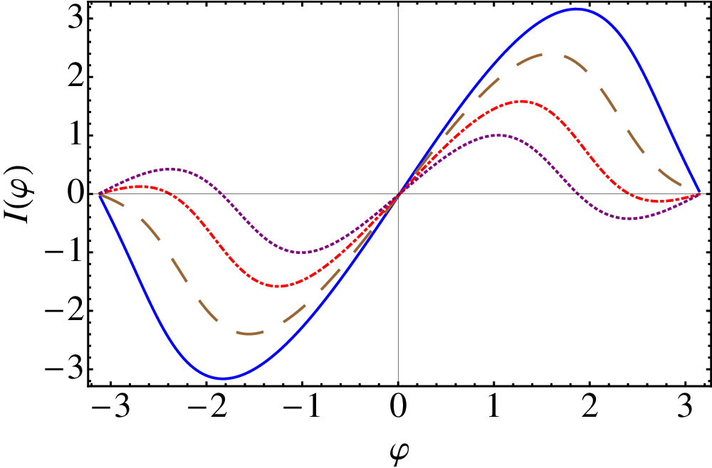
in the CPR is observed. This is perfectly consistent with the plots we show in Fig. 3,
where we assume , with being the angle between the (in-plane) magnetization
and the x axis, that is, – see appendix A for
details. To spell our why the anomaly is zero when , let
us consider the unitary operator , defined as
,
with being the parity operator in the y direction, that is,
. By direct calculation, one readily checks that,
with the system Hamiltonian in Eq. 1 (and, more
generically, with any Hamiltonian envisaging a parabolic confinement in the y direction),
one obtains
(note that, for the sake of the discussion, in the above equation we explicitly show the
dependence of on , as well). Thus, we infer that, if
has an energy eigenvalue , then must have an energy
eigenvalue with the same energy (but opposite values of the parameters and ).
As a result, at zero temperature, the groundstate energy of the system must be invariant under
and, accordingly, once taking the derivative
of the groundstate energy with respect to , one obtains . Setting (which is equivalent to assuming that
the magnetization is perpendicular to the SO field), we eventually obtain that
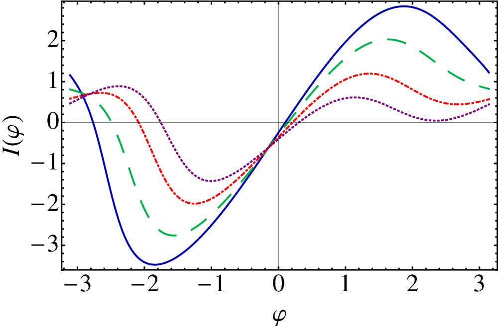
for .) Rotating the magnetization towards the SO field results in two effects:
i) the appearance of an anomaly in the CPR (),
ii) the appearance of a nonzero asymmetry ().
In general, discontinuities may appear in the plots of vs. , wich are typically due to crossings between Andreev levels. Nevertheless, for the sake of the presentation, in Figs. 2,3 we have chosen a set of parameters such that no discontinuities appear in the CPR. Also, we stress that, for both cases in Fig. 2 and Fig. 3, higher values of the exchange field correspond to a smaller amplitude of the Josephson current accompanied by faster oscillations as a function of . To explain those features, we note that, on the one hand, the reduction in the amplitude can be ascribed to the effect of the magnetic region which acts as spin filter, effectively reducing the transmission of one spin species and consequently reducing the efficiency of Cooper pair transfer between the two superconducting leads. On the other hand, the appearance of high order harmonics in the CPR for higher values of the exchange field appears to be a precursor of a transition.
To evidence how depends on the system parameters, in Fig. 4 we show , defined as the phase at which the Josephson energy is minimum (and, accordingly, ), calculated for several values of the SOI of and of the exchange field of . The parameters employed to generate the plots are reported in the figure’s caption. To perform a similar analysis for the asymmetry, we therefore use the quantity and, plot as a function the SOI and the exchange field in Fig. 5. As a main comment, it is worth pointing out that when the angle between the exchange field and the SO field is zero. As it is evident from Fig. 4 and Fig. 5 larger values of the SOI and the exchange field correspond to larger values of and , if the exchange field is properly oriented with respect to the spin-orbit field. In order to study whether it is possible to enhance and without resorting to larger values of the fields in the next section we analyze a multi-layer setup with two spin-orbit coupled and two ferromagnetic regions.


III.2 4 Regions
We now move to discuss the setup represented in Fig. 6, in which the normal region consists of four different sections, with alternating SOI coupled and ferromagnetic regions. Again we calculate the scattering matrix of each region and then after translating them to the proper position we construct the full scattering matrix, as previously explained. In order to compare the results of this subsection to those of the previous one we, assume that the total length of the two spin-orbit coupled (ferromagnetic) region is equal to that of the single spin-orbit (ferromagnetic) region in the two-region setup. In this way we can assess whether, and to what extent, increasing the number of layers works to maximize the anomaly in the CPR, as well as to recover a larger values of , that is, to obtain a larger superconducting rectifying affect.
Here, to avoid further complications, we take the orientation of the exchange field in the two ferromagnetic regions to be along the y direction, i.e. orthogonal to the spin-orbit field. In principle one might allow for different orientation of the exchange field in the two ferromagnetic regions but, possibly, the case addressed below corresponds to the most accessible configuration in real devices. Notwithstanding the difficulty of orienting the exchange field in the two ferromagnetic regions, in light of the results of Ref. 28 it would be reasonable to expect that larger values of and can be obtained by fine tuning the angle between the magnetizations.
By analyzing the CPR for several values of the spin-orbit coupling and the magnetization, as well as changing the relative magnitude of () and (), we find the that the magnitude of is in general of the same order of magnitude for the two- and the four-regions setups. Conversely, and most importantly for future applications, we find that the asymmetry between and in the four-regions setup can be enhanced to the two-regions one by an asymmetric choice of the lengths of the different sections. Indeed, as we show in Fig. 7 in the four region setup for the regions of parameters considered, we find maximum values of , whereas for the two region setup we obtain at most . This result would suggest that multilayer heterostructure as the one studied here may be useful in designing rectifying superconducting devices.


IV Random matrix analysis
In this section, we discuss how our results about AJE and nonzero asymmetry are related to the total number of open channels that we take into account. As we pointed out before, we are interested in setting the system parameters so to maximize both and the critical current asymmetry. By direct calculation (not illustrated here), we found when , while, to find , we have to set . To the best of our knowledge, there is no a priori reason why only for one should have . Thus, in order to understand whether this finding is accidental to our model, or it rather occurs in general we have performed a numerical simulation using random scattering matrices to describe the normal region (note that resorting to random scattering matrices is a standard mean to deal, for instance, with dephasing effects in mesoscopic systems [46, 47]). Specifically, we assume that the two superconducting leads are connected to each other by a normal region characterized by a scattering matrix . We take to be a unitary matrix, whose elements are extracted with an uniform probability distribution, with no further restriction. Since we look for Josephson junctions which exhibit anomalies in the Josephson CPR, we do not enforce symmetries on the matrix , such as time reversal, or spin-rotational symmetry[48]: in fact, in the presence of either one of these latter symmetries (or of both of them), would belong respectively to the orthogonal and to the symplectic group. Using symmetry arguments it can be shown that for these two symmetry classes [8, 9]. By means of Eq. 15, we therefore calculate the Andreev spectrum and the Josephson current, computing then and for each random realization. To quantify the asymmetry, we use the mean square visibility , with for a given scattering matrix, and denoting the average over a large number of different realization of the random matrix. We repeat the calculation for the number of open transport channels . For each case we generate random scattering matrices and, using Eq. 15, we compute the Andreev spectrum and the Josephson current and, eventually, we compute for each realization of .


In Fig. 8 we plot the computed value of as a function of the number of realizations. We find that for , so that only a small asymmetry can be observed in this case, in accordance with our calculation using the Hamiltonian of Eq. 5. Moreover, non-zero values of are found only for realization of such that the CPR is discontinuous. For the case we find and the asymmetry can be observed even for a continuous CPR. It should be stressed that, within the approach presented here, we are properly describing the Josephson effect through a cavity and not the case of a wire[48, 49]; the latter case will be the subject of a further study.
V Summary and Outlook
In this work we have demonstrated that the anomalous Josephson effect can be expected in SNS junctions where the normal region in a heterostructure formed by alternating ferromagnetic and spin orbit coupled segments. We have shown that when the Fermi energy is such that the number of transport channels it is possible to observe a sizeable direction dependency of the critical current; we have validated this result also using a random matrices analysis. Moreover we have shown that the asymmetry between and can be enhanced using a four layer heterostructure vs a two layer one. Our findings might be relevant to the design of devices with large , asymmetry to be employed as diodes in superconducting circuits.
Appendix A Calculation of the Scattering matrix
In this appendix, we outline the calculation of the -matrix for the normal region. In view of the relation , by means of the same token, we compute the -matrix for the normal region, as well. In practice, we first divide the normal region in a SOI and a ferromagnetic segment and separately derive the scattering matrices of the two regions, respectively referred to in the following as and . Eventually, we combine the two of them to calculate the -matrix for the whole normal region. In fact, apart for the technical subtelties in combining together and , our approach appears to be particulary convenient, as it allows us to generalize our study to multi-layer setups. To combine together and , it is more convenient to resort to the transfer matrices, for which a simple composition rule exists. To do so, we decompose each scattering matrix into reflection and transmission blocks, according to
| (17) |
Next, we introduce the transfer matrices and . By definition, each relates the scattering amplitudes to the left-hand side of the corresponding region to the ones at the right-hand side, according to
| (18) |
with denoting the scattering amplitudes across the corresponding scattering regions. In analogy with the scattering matrices, the transfer matrices admit a block decomposition, as well, according to
| (20) |
together with their inverse
| (21) |
To derive the transfer matrix, we separately solve the Schrödinger equation in the various normal regions by setting at the center of each region. Eventually, using the composition law of the transfer matrices, we shift the corresponding matrices according to their location within the heterostructure and combine them to obtain the total transfer matrix as . From the total transfer matrix we then calculate the full scattering matrix, which we use to compute the Andreev spectrum.
A.0.1 Scattering matrix of spin-orbit coupled region
We begin our calculation by deriving . To do so, by standard methods, we explicitly solve the Schrödinger equation in the spin-orbit region and at its left- and right-hand side, where only transverse confinement is assumed. Eventually, we match the solutions at the interfaces. When doing the corresponding calculations, we let the Fermi energy vary in an interval such that only two transport channels are open, each with two spin orientations.
The wave functions corresponding to the scattering states at energy to the left- and to the right-hand side of the SOI region can be readily written as
| (22) |
with and the -sign referring to the right-going and to the left-going states. In Eq. 22, and are respectively the eigenfunctions of the harmonic oscillator and of the spin Pauli matrix . In particular, we label the groundstate of the harmonic oscillator with , the first excited state with , and so on. Moreover, we set and . At variance, for , there are no propagative solutions and the corresponding (evanescent) modes are described by the wave functions
| (23) |
with , where the + (-) sign refers to the left-hand side (right-hand side) region.
To obtain the eigenfunctions in the SOI region, we numerically diagonalize the Hamiltonian using the basis . For simplicity we truncate the Hilbert space considering the first three sub-bands, resulting in a Hamiltonian matrix. Such an approximation is expected to give a reasonable description of the system even in the presence of a sizeable SOI[37]. Accordingly, our problem is now reduced to finding the eigenvalues and the eigenfunction of the corresponding -finite dimensional Hamiltonian matrix . For a given energy E, the allowed are obtained from the equation
| (24) |
which implies that, for each value of the energy we have 12 solutions , with the corresponding eigenfunctions given by:
| (25) |
where the coefficients have to be determined numerically, while the coefficients are determined by imposing the proper matching conditions, as discussed below. For two open transport channels in the leads, each one with both spin polarizations, the electronic scattering matrix takes the form:
| (26) |
with the () block given by
| (27) |
and similar expressions for and . To move ahead in the calculation, one has to compute all the reflection and transmission coefficients, by matching the wave function in Eq. 25 with the one in the leads, for any possible choice of scattering boundary conditions. To illustrate how the procedure works, let us explicitly discuss the case of a spin-up particle incoming from the left-hand side. In this case, the wave functions within the left-hand side () and the right-hand side () are respectively given by:
| (28) |
| (29) |
Let us denote with the total length of the SOI region and, to simplify the derivation, let us assume that the interfaces are symmetrically located at . The matching conditions at the interfaces require that the wave function is continuos while, in general, its derivative with respect to must be discontinuous, to account for the discontinuous SOI interaction (cfr. Eq. 5). Projecting the equations corresponding to the matching conditions onto the basis states () we obtain the following set of equations:
| (30) |
| (31) |
| (32) |
| (33) |
Therefore, we have a set of equations which we solve numerically to determine the corresponding matrix elements. Repeating the calculation for each possible incoming channel we construct as a function of the energy . Eventually, consistently with the above discussion, we set .
A.0.2 Scattering matrix of the ferromagnetic region
The calculation of is quite simpler, since, in this case, it is straightforward to explicitly solve the Schrödinger equation and to find the corresponding eigenvalues and eigenfunctions. In the case of in-plane magnetization, corresponding to the unit vector , the eigenfunctions are given by
| (34) |
with spinors in the spin space, . From the wavefunctions in Eq. 34 it is now straightforward to compute by exactly the same procedure we have used to derive , which is even more simplified by the fact that the wave functions and their derivatives are both continuous at the interfaces.
A.0.3 Translation of the Scattering potential
For convenience, in computing and , we have assumed that the corresponding regions were symmetric with respect to the origin of the -axis. Now, when composing the results to construct the full -matrix, we need to translate the center of scattering regions to its proper position, so that i.e. the SO region ranges between and and the F region between and (a pertinent generalization of such a procedure will lead us to correctly approach, in the following, a sandwich-like structure with more than two regions).
To illustrate our procedure, let us consider a scattering matrix , determined by some potential , defined so that
| (35) |
with the block decomposition of Eq. 26 for . Assuming, as we have done throughout our paper, that an equal number of transport channels is available at the left-hand side and at the right-hand side of the scattering region, the blocks will be realized as matrices. Let be the scattering potential obtained by translating by a distance d along the x-axis and let and be the solutions of the Schrödinger equation respectively corresponding to and to respectively, so that one has . Making use of this last relation, it is straightforward to show that the scattering matrix relative to can be obtained from by the following transformation:
| (36) |
with . In terms of the blocks of the scattering matrix we have:
| (37) |
and similarly for the transfer matrix
| (38) |
References
- [1] H. O. H. Churchill, V. Fatemi, K. Grove-Rasmussen, M. T. Deng, P. Caroff, H. Q. Xu, and C. M. Marcus, Phys. Rev. B 87, 241401 (2013).
- [2] E. J. H. Lee, X. Jiang, M. Houzet, C. M. Aguado, R. and Lieber, and S. De Franceschi, Nature Nanotechnology 9, 79 (2013).
- [3] J. Alicea, Reports on Progress in Physics 75, 076501 (2012).
- [4] B. Douçot, M. V. Feigel’man, and L. B. Ioffe, Phys. Rev. Lett. 90, 107003 (2003).
- [5] D. Giuliano and P. Sodano, EPL (Europhysics Letters) 88, 17012 (2009).
- [6] T. Yokoyama, M. Eto, and Y. V. Nazarov, Phys. Rev. B 89, 195407 (2014).
- [7] A. Barone and G. Paternó, Physics and applications of Josphson effect (Wiley, 1982).
- [8] T. Yokoyama, M. Eto, and Y. Nazarov, J. Phys. Soc. Jpn. 82, 054703 (2013).
- [9] G. Campagnano, P. Lucignano, D. Giuliano, and A. Tagliacozzo, Journal of Physics: Condensed Matter 27, 205301 (2015).
- [10] V. B. Geshkenbein and A. I. Larkin, JETP Lett. 43, 395 (1986).
- [11] S. Kashiwaya and Y. Tanaka, Reports on Progress in Physics 63, 1641 (2000).
- [12] M. Sigrist, Progress of Theoretical Physics 99, 899 (1998).
- [13] S. Yip, Phys. Rev. B 52, 3087 (1995).
- [14] R. Grein, M. Eschrig, G. Metalidis, and G. Schön, Phys. Rev. Lett. 102, 227005 (2009).
- [15] Y. Tanaka, A. A. Golubov, S. Kashiwaya, and M. Ueda, Phys. Rev. Lett. 99, 037005 (2007).
- [16] A. Buzdin, Phys. Rev. Lett. 101, 107005 (2008).
- [17] Y. Asano, Y. Tanaka, M. Sigrist, and S. Kashiwaya, Phys. Rev. B 67, 184505 (2003).
- [18] M. Eschrig and T. Lofwander, Nature Physics 4, 138 (2008).
- [19] Y. Asano, Y. Sawa, Y. Tanaka, and A. A. Golubov, Phys. Rev. B 76, 224525 (2007).
- [20] V. Braude and Y. V. Nazarov, Phys. Rev. Lett. 98, 077003 (2007).
- [21] F. Konschelle and A. Buzdin, Phys. Rev. Lett. 102, 017001 (2009).
- [22] A. Zazunov, R. Egger, T. Jonckheere, and T. Martin, Phys. Rev. Lett. 103, 147004 (2009).
- [23] A. Brunetti, A. Zazunov, A. Kundu, and R. Egger, Phys. Rev. B 88, 144515 (2013) 88 (2013).
- [24] A. A. Reynoso, G. Usaj, C. A. Balseiro, D. Feinberg, and M. Avignon, Phys. Rev. Lett. 101, 107001 (2008).
- [25] A. A. Reynoso, G. Usaj, C. A. Balseiro, D. Feinberg, and M. Avignon, Phys. Rev. B 86, 214519 (2012).
- [26] I. V. Krive, L. Y. Gorelik, R. I. Shekhter, and M. Jonson, Low Temperature Physics 30, 398 (2004).
- [27] I. V. Krive, A. M. Kadigrobov, R. I. Shekhter, and M. Jonson, Phys. Rev. B 71, 214516 (2005).
- [28] M. A. Silaev, I. V. Tokatly, and F. S. Bergeret, Phys. Rev. B 95, 184508 (2017).
- [29] K. N. Nesterov, M. Houzet, and J. S. Meyer, Phys. Rev. B 93, 174502 (2016).
- [30] P. Marra, R. Citro, and A. Braggio, Phys. Rev. B 93, 220507 (2016).
- [31] C. Schrade, S. Hoffman, and D. Loss, Phys. Rev. B 95, 195421 (2017).
- [32] D. B. Szombati, S. Nadj-Perge, D. Car, S. R. Plissard, E. P. A. M. Bakkers, and L. P. Kouwenhoven, Nat Phys 12, 568 (2016).
- [33] L. Fidkowski, J. Alicea, N. H. Lindner, R. M. Lutchyn, and M. P. A. Fisher, Phys. Rev. B 85, 245121 (2012).
- [34] I. Affleck and D. Giuliano, Journal of Statistical Mechanics: Theory and Experiment 2013, P06011 (2013).
- [35] I. Affleck and D. Giuliano, Journal of Statistical Physics 157, 666 (2014), ISSN 1572-9613.
- [36] A. Rasmussen, J. Danon, H. Suominen, F. Nichele, M. Kjaergaard, and K. Flensberg, Phys. Rev. B 93, 155406 (2016).
- [37] M. Governale and U. Zülicke, Phys. Rev. B 66, 073311 (2002).
- [38] V. Ramaglia, D. Bercioux, V. Cataudella, G. D. Filippis, and C. Perroni, J. Phys.: Condens. Matter 16, 9143 (2004).
- [39] K. K. Likharev, Rev. Mod. Phys. 51, 101 (1979).
- [40] F. Bloch, Phys. Rev. B 2, 109 (1970).
- [41] D. Giuliano and I. Affleck, J. Stat. Mech. p. P02034 (2013).
- [42] D. Giuliano and I. Affleck, Phys. Rev. B 90, 045133 (2014).
- [43] A. Nava, R. Giuliano, G. Campagnano, and D. Giuliano, Phys. Rev. B 94, 205125 (2016).
- [44] C. W. J. Beenakker, Phys. Rev. Lett. 67, 3836 (1991).
- [45] C. Beenakker, in Transport phenomena in mesoscopic systems, edited by H. Fukuyama and T. Ando (Springer, Berlin, 1992).
- [46] C. W. J. Beenakker, Rev. Mod. Phys. 69, 731 (1997a).
- [47] P. Lucignano, D. Giuliano, and A. Tagliacozzo, Phys. Rev. B 76, 045324 (2007).
- [48] C. W. J. Beenakker, Rev. Mod. Phys. 69, 731 (1997b).
- [49] G. Campagnano and Y. V. Nazarov, Phys. Rev. B 74, 125307 (2006).