Tuning the Aharonov-Bohm effect with dephasing in nonequilibrium transport

The Hamiltonian describing the system reads

where

The system $H_{\rm s}$ is coupled to the electronic reservoirs $H_{\rm r}$ and heat bath $H_{\rm b}$ via the Hamiltonians $H_{\rm s,r}$ and $H_{\rm s,b}$. The coupling between system and electronic reservoirs $H_{\rm s,r}$ is assumed to be weak so that an application of the Redfield equation with Born-Markov approximation is valid, but we allow for a strong coupling between system and heat bath $H_{\rm s,b}$. The operators $\hat{a}_{n}$, $\hat{c}_{n,k}$ shall fulfill fermionic commutation relations, while $\hat{b}_{n,k}$ are bosonic operators. The term $H_{\text{int}}$ describes the Coloumb interaction of two particles, which is assumed to be so strong that at most one particle can be in the system. For this reason, this term is not further specified.

The AB effect in a tight-binding model can only appear in a ring geometry. Let us consider a parameterization of the internal system coupling parameters $J_{n,m}=J_{n,m}^{(0)}e^{i\phi_{n,m}}$ with real $J_{n,m}^{(0)}$ and $\phi_{n,m}$. The coupling between the reservoirs and the system is parameterized accordingly, namely $W_{n,k}=W_{n,k}^{(0)}e^{i\varphi_{n,k}}$ with real $W_{n,k}^{(0)}$, $\varphi_{n,k}$. The phase factors $e^{i\varphi_{n,k}}$ can be transformed away by gauge transformations $\hat{c}_{n,k}\rightarrow\hat{c}_{n,k}e^{-i\varphi_{n,k}}$, rendering $W_{n,k}$ real valued. However, if all $J_{n,m}^{(0)}\neq 0$, it is not possible to completely render the coupling parameters $J_{n,m}$ real valued by gauge transformations. In contrast, the phase

can be proven to be invariant under transformations $\hat{a}_{n}\rightarrow\hat{a}_{n}e^{-i\tilde{\phi}_{n}}$ for arbitrary $\tilde{\phi}_{n}$. The phase $\phi$ is thus a gauge-invariant quantity and has physical relevance, i.e., the energies and the eigenstates of the Hamiltonian depend on $\phi$. This is the underlying reason for the famous AB effect. In contrast, if the ring is broken, i.e., $J_{n,m}^{(0)}=0$ for one coupling, the phases can be removed. For example, such a phase $\phi$ appears if there is a magnetic field perpendicular to the ring [42]. More precisely, the phase can be expressed in terms of a magnetic field as $\phi=\frac{e}{h}\cdot B_{\rm n}\cdot A$, where $B_{\rm n}$ is the component of the magnetic field normal to the ring, $A$ is the ring area and $\frac{h}{2e}=2,068\cdot 10^{-15}\rm\,Tm^{2}$ is the magnetic flux quantum. For a notational reason, we define $J_{n}=J_{n,n+1}^{(0)}$, where $n=4$ corresponds to $n=1$.

A dark state denotes an eigenstate at which the wave function on one site of the local basis vanish completely due to destructive interference. Because of this outstanding property, dark states have been suggested as quantum memory [43] and are related to electromagnetically-induced transparency [44, 45, 14, 15].

If two onsite energies $\epsilon_{n}$ are equal, $J_{n}=J$ and $\phi=0,\pi$, then the system can be easily diagonalized due to the appearance of a dark state. Assuming, e.g., $\epsilon_{1}=\epsilon_{3}$, we find the eigenstates

with energies $E_{0,\pi}^{\text{dark}}=\epsilon_{3}\mp J,$ for $\phi=0,\pi$, respectively. The wave function is valid for the gauge choice of $\phi_{1,2}=\phi_{2,3}=0$ and $\phi_{3,1}=0,\pi$. As these states have no overlap with site $n=2$, they are indeed dark states, which have an essential influence on the transport properties.

To probe experimentally accessible quantities, we focus on the steady-state electronic current of particles entering reservoir $n=2$ in the long-time limit of $t\rightarrow\infty$, the corresponding noise, and the waiting-time statistics.

We take advantage of the polaron-transformed Redfield equation [46, 47, 48]. The polaron transformation is defined by a unitary transformation

Details can be found in Appendix A. The polaron transformation modifies the Hamiltonian Eq. (2) as follows:

with

Here, $\kappa$ is a renormalization parameter, which captures the influence of the strongly coupled bath on the system, i.e., the onsite energy of site $n=3$ gets renormalized. As explained in Sec. II.2, the constrain $\epsilon_{3}=\epsilon_{1}$ is a requirement for the appearance of the dark state. Yet, due the coupling to the heat bath, this condition has to be fulfilled by $\epsilon^{\prime}_{3}$. In order to simplify our analysis, we investigate the system as a function of $\epsilon^{\prime}_{3}$, so that we can directly control the appearance of the dark state.

Importantly, the polaron transformation renders the coupling to the bath $H_{\rm s,b}^{(p)}$ weak in comparison to the system parameters, so that the application of the common Redfield equation formalism is justified [49]. In doing so, we obtain equations of motions for the reduced density matrix of the system $\rho=\text{ Tr}_{\text{ br }}\left(\rho_{\text{tot}}\right)$, where $\rho_{\text{tot}}$ denotes the density matrix of the system plus the reservoirs and the bath, and $\text{ Tr}_{\text{ br}}\left(.\right)$ denotes a trace over the bath and reservoirs’ degrees of freedom. The equation of motion of the reduced density matrix finally reads

where $\mathcal{W}$ is a time-independent matrix and denotes the Liouvillian superoperator. Details of the derivation can be found in Appendix B. This approach can describe both, incoherent and coherent processes [47], similar to the method considered in Ref. [50]. In contrast to Ref. [51], the polaron transformation allows to study the influence of decoherence even for strong couplings $\gamma$.

Equation (10) can be amended to take account of transport statistics. In doing so, we consider the conditioned density matrix $\rho(t,\mathbf{N})$ with $\mathbf{N}=(N_{1},N_{2})$ of the central system, which contains additional information about the number of particles $N_{n}$ in reservoir $n=1,2$. To this end, we unravel Eq. (10) as

where $\mathcal{W}_{0}$ describes a time evolution with no particle jumps from or to the reservoirs. The superoperators $\mathcal{W}_{\sigma}^{n}$ add $(\sigma=1)$ or remove $(\sigma=-1)$ a particle to the system, while correspondingly remove or add it to the reservoir $n$. The quantity $\mathbf{N}^{(n,\sigma)}$ is equal to $\mathbf{N}$ but with $N_{n}$ replaced by $N_{n}+\sigma$.

Applying a Fourier transformation in the particle space $\mathbf{N}=(N_{1},N_{2})$, the generalized reduced density matrix $\rho(t,\boldsymbol{\chi})$ fulfills the equation of motion

where $\boldsymbol{\chi}=(\chi_{1},\chi_{2})$ are the variables conjugated to $\mathbf{N}$. The current and the frequency-dependent noise can be calculated using

where $\mathcal{J}_{n}^{(m)}\equiv\partial_{\chi_{n}}^{m}\mathcal{W}(\boldsymbol{\chi})$ and $\Omega_{0}(z)\equiv\left[z-\mathcal{W}_{0}\right]^{-1}$ [52, 53].

As we see later, the statistical distribution $P^{(n,n^{\prime})}(\tau)$ of the time difference $\tau$ between two consecutive jump events $\mathcal{W}_{\sigma=1}^{n}$ and $\mathcal{W}_{\sigma^{\prime}=-1}^{n^{\prime}}$ contains interesting information about the system dynamics [54]. This waiting-time experiment is sketched in Fig. 1(b). At time $t=t_{0}$, a particle enters the system from reservoir $n$. The waiting time distribution describes the probability that the particle jumps into reservoir $n^{\prime}$ at time $t_{1}=t_{0}+\tau$. In between, the dynamics is governed by the internal properties of the system. Thus, the waiting time distribution can provide insight to the AB effect and the dephasing dynamics.

According to Ref. [55], the waiting-time probability distribution can be calculated using

where $\rho_{s}$ denotes the steady states of the system with $\dot{\rho}_{s}=0$ for the dynamics in Eq. (10). The denominator ensures the normalization

Single-electron resolution in transport has been achieved in single-electron transistor experiments such as in Refs. [18, 19]. Moreover, waiting-time distributions have been suggested to reveal the interplay of the electronic and vibrational degrees of freedom in molecular junctions [56].

In Fig. 2, we plot the stationary current as a function of the phase $\phi$ for different system parameters. In Fig. 2(a), we focus on the influence of the system-bath coupling, characterized by the spectral coupling density

where we have chosen a super-Ohmic parametrization with cut-off frequency $\omega_{c}$.

For the coupling strength $\gamma=0$ we observe that the current $I_{s}$ sensitively depends on the phase $\phi$. It is interesting to see that the current exhibits a local minimum at $\phi=0$, while the maximum current is reached here for finite phases $\phi=\pm\phi_{\text{m}}$ for the chosen chemical potential of $\mu_{1,2}$. In other words, transport can be enhanced with the help of the AB effect, i.e., $\phi\neq 0$.

As the system-bath coupling strength $\gamma$ increases, the $\phi$ dependence of the current becomes weaker. A rough explanation of this behavior is that the AB effect is based on the coherent wave nature of the charge, i.e., the interference of the two pathways. Due to the increasing coupling to the thermal bath, thermal fluctuations increasingly destroy the coherent dynamics. This behavior can be observed in Fig. 2(b), where a raising temperature leads to enhanced thermal fluctuations, which suppress the coherent system dynamics and consequently the $\phi$ dependence.

The phase dependence of the current can be understood as follows. According to the Redfield equation with the Born-Markov secular approximation, the expression for the current through the system can be written as

where

denotes the transition rates from the vacuum state to the eigenstates $\left|\lambda\right>$ with energy $E_{\lambda}$, induced by reservoir $n$. $P_{0}$ denotes the probability that the system is in the vacuum state. Here, $f_{n}(E)$ is the Fermi distribution in reservoir $n$ and $\Gamma_{n}(\omega)=\Gamma_{n}^{(0)}\omega_{\text{c},n}^{2}/\left[(\omega-\omega_{0,n})^{2}+\omega_{\text{c},n}^{2}\right]$.

In appendix C we show that the current through the eigenstate $\left|\lambda\right>$ in Eq. (19) can be written as

This expression illustrates the $\phi$ sensitivity and its dependence on the thermal fluctuations. For an increasing system-bath coupling $\gamma$ or for a large temperature $T_{3}$, the tunneling parameters are renormalized as $J_{2}\rightarrow\kappa J_{2}$ and $J_{3}\rightarrow\kappa J_{3}$ according to Eq. (6). For larger $\gamma$ or $T_{3}$ the polaron renormalization parameter $\kappa$ approaches $0$. In that limit, it is clear from Eq. (6) that the coherence in the polaron-transformed Hamiltonian is suppressed so that the AB effect vanishes. Accordingly, in Eq.(21) we find that the $I_{s}^{(\lambda)}$ dependence on $\phi$ vanishes. A similar reasoning applies to the factor $\mathcal{N}_{\lambda}$. The thermal bath can thus be used to tune the AB effect and the related time-reversal symmetry breaking. This is thus reminiscent to the breaking of spatial symmetries with dephasing as investigated in Ref. [57].

From Eq. (21) it is hard to determine the optimal phase $\phi_{\text{m}}$ for the maximum current as the $\phi$ dependence of $\mathcal{N}_{\lambda}$ is complicated, as shown in appendix C. Moreover, Eq. (21) reveals that the current strongly depends on the onsite potential $\epsilon^{\prime}_{3}$. In Fig. 2(c) we depict the phase dependence of the current for different values of $\epsilon^{\prime}_{3}$. The $\phi$ dependence is most significant if $\epsilon^{\prime}_{3}$ is on the same order as $\epsilon_{1}$ and $\epsilon_{2}$. If $\epsilon^{\prime}_{3}$ is detuned from the other onsite-energies, the site $n=3$ is hard to reach for a charge initially located at one of the other sites. For this reason, the intra-ring coherence and therefor the AB effect is weakened. Also the $\phi$ dependence looks different depending on $\epsilon^{\prime}_{3}$. For a large (small) $\epsilon^{\prime}_{3}$, we observe a minimum (maximum) current $\phi=0$, and a maximum (minimum) current at $\phi=\pi$. For $\epsilon^{\prime}_{3}\approx\epsilon_{1},\epsilon_{2}$, the maximum current is found at finite $\phi=\pm\phi_{\rm m}$ and exhibits a local minimum at $\phi=0$. Thus, by tuning $\epsilon^{\prime}_{3}$, one can control the current-phase dependence.

Furthermore, in Fig. 2(d) we find that by adjusting the phase $\phi$, we can generate distinct $\epsilon^{\prime}_{3}$ dependencies for the current. For all $\phi$ we observe that the current for small $\epsilon^{\prime}_{3}$ is lower than for large $\epsilon^{\prime}_{3}$. This happens as we allow here only for single-electron occupation of the system: If $(\epsilon^{\prime}_{3}\ll\epsilon_{1},\epsilon_{2})$ or $(\epsilon^{\prime}_{3}\gg\epsilon_{1},\epsilon_{2})$ then there is an eigenstate strongly localized at $n=3$. For $(\epsilon^{\prime}_{3}\ll\epsilon_{1},\epsilon_{2})$ this state is likely occupied with a charge, so that the transport is blocked. For $(\epsilon^{\prime}_{3}\gg\epsilon_{1},\epsilon_{2})$, the localized state is likely to be empty, so that the transport properties are determined by the coherent transition from sites $1\rightarrow 2$. In particular, for $\phi=0$ we observe a non-monotonic dependence on $\epsilon^{\prime}_{3}$. This can be explained with the appearance of a dark state as explained in the following subsection.

The current characteristics can be explained following the arguments in Ref. [58]. It is strongly related to the appearance of the dark state as described in Sec. II.2. Inserting the energy for the dark state $E^{\rm dark}_{0,\pi}$ below Eq. (5) into the partial current expression Eq. (21) for $\phi=0,\pi$, we find that $I_{s}^{(\lambda)}=0$, i.e., the dark state does not contribute to the current. Upon tuning the phase away from $\phi=0$ or $\pi$, the dark state disappears, so that all eigenstates contribute to the current. Thus, the dark state may give rise to a suppression of the transport.

To understand this in detail, we depict in Fig. 3(a) the spectrum $E_{\lambda}$ of the polaron-transformed system Hamiltonian, and in Fig. 3(b) the occupation of the corresponding eigenstates $\lambda$. The dark states appear for $\phi=0$ and $\phi=\pi/2$ in eigenstate $\lambda=1$ and $\lambda=2$, respectively. Both are energetically located on a local maximum of $E_{\lambda}(\phi)$. For this reason, one might conclude, that they are less thermally occupied in comparison to the other $\phi$ values. Yet, as we observe in Fig. 3(b), the occupation $n_{\lambda}$ of the eigenstate $\lambda$ exhibits a local maximum, as the dark state Eq. (5) is only coupled to reservoir $n=1$, but not to reservoirs $n=2$. Thus, a charge occupying the dark state can neither enter reservoir $n=1$, because all orbitals are almost occupied due to the chosen chemical potential $\mu_{1}$, nor can it enter reservoir $n=2$, as the dark state has no overlap with site $n=2$. This leads to an enhanced occupation of the dark state and to a blockade of the transport.

The presence of a dark state explains the dependence of the current on $\phi$ and $\epsilon^{\prime}_{3}$, in Fig. 2(a) and (d). As the dark state only appears at singular parameter combinations, e.g., $\phi=0$ and $\epsilon^{\prime}_{3}=\epsilon_{1}$, the current shows a decrease when the system parameters approach the dark state configuration. In Fig. 2(d), the influence of the dark state is not as prominent for $\phi=\pi$ as for $\phi=0$, because the dark state energy $E^{\text{dark }}_{\pi}=\epsilon_{1}+J$ is above the transport window $E^{\text{dark }}_{\pi}>E\in(\mu_{2},\mu_{1})$. Nevertheless the current for $\phi=\pi$ is significantly smaller than the current for $\phi=\pi/2$, which is a consequence of the dark state.

We emphasize that the dark state blockade and the minimum in the transmission observed in the molecular transport experiment [38] are both based on destructive interference of different charge paths. The experiment demonstrates that the electronic transport occurs essentially via three localized molecular orbitals, so that it is strongly related to our model system. Furthermore, interference experiments related to dark states have interesting applications such as the interaction free measurements using anti-resonances in optical and solid-state systems, which are also feasible to coherently detect dissipation [59, 60, 61].

In an experimental investigation, the response of the current due to a change of the magnetic field is important. To this end, we define a figure of merit by

which we depict, scaled by the ring area $A$, in Fig. 4. Here we use the same parameters as in Fig. 2(a), and we choose an experimentally realistic reservoir coupling of $\Gamma_{n}^{(0)}=10\,\rm kHz$ [18]. From Fig. 2(a) we can thus conclude that $I_{\rm s}(\phi\approx 0.5)\approx 500\frac{1}{\rm s}$. In the following we discuss two examples.

A semiconductor quantum dot (or single electron transistor) has a characteristic size of $1\rm\mu m$, so that the area of a triple quantum dot is in the order of $A=1\rm\mu m^{2}$. $\phi=0.5$ corresponds to a magnetic field of $B_{\rm n}\approx 0.3\,\rm mT$. From Fig. 4, we find that for this magnetic field the figure of merit is $F=6\times 10^{5}\frac{1}{\rm sT}$, so that an increase of $\Delta B_{n}=0.01\,\rm mT$ gives rise to a current change of $\Delta I_{s}\approx 6\frac{1}{\rm s}$. This can be measured in experiments [18].

Molecules can have ring structures with area $A\approx 1\,\rm nm^{2}$, so that a magnetic field of $B_{\rm n}=300\,\rm T$ is needed to acquire a phase of $\phi=0.5$. However, the largest artificially generated continuous magnetic field is nowadays $B_{n}=45\,\rm T$ [62]. Thus, the values $\phi\approx 0,\pi$ in our model refer to interference phenomena in molecular ring structures, such as experimentally investigated in Ref. [38, 39]. Our investigation based on the polaron transformation helps to reveal the impact of dephasing on the interference in molecular setups, where the coupling between electronic and vibronic degrees of freedom is crucial.

Although the current shows a strong dependence on the phase $\phi$, it is symmetric regarding the inversion $\phi\rightarrow-\phi$. This symmetry is denoted as phase rigidity [9]. It is related to the fact that the current is not sensitive to the details of the coherent dynamics of the system. To get more information about the internal dynamics, the frequency dependent noise Eq. (14) is a more appropriate observable. We depict the noise in Fig. 5 as a function of $\phi$ and $\omega$. We observe a mainly frequency independent pattern which results from the $\mathcal{J}^{(2)}_{n=2}$ operator in Eq. (14). On top of that, we observe a frequency-dependent structure. This structure resembles the energy differences of the eigenstates $\Delta E_{\lambda\mu}=E_{\lambda}-E_{\mu}$, which we depict in Fig. 5 with dashed lines. Although it thus gives information about the internal structure of the system, it nevertheless exhibits a $\phi\leftrightarrow-\phi$ symmetry.

We stress that the phase rigidity is a consequence of the fact that our system exhibits two electronic reservoirs. It is well-know that the phase rigidity in the stationary current is broken when increasing the number of electronic reservoirs, as experimentally demonstrated in Ref. [25, 26]. In contrast, the third terminal in our system is a heat bath, which does not break the phase rigidity, even not for strong coupling, as demonstrated here.

In contrast to the stationary current and its noise, the waiting time statistics as defined in Eq. (15) indeed violates the $\phi\leftrightarrow-\phi$ symmetry, similar to the transient current investigated in Ref. [9]. Figure 6 shows instances of time evolutions for $\phi=0,\pm\pi/2$. In Fig. 6(a)-(c) we plot the occupations of the sites $N_{n}$ for $n=1,2,3$ by a particle which has jumped at time $t=t_{0}$ from reservoir $n=1$ into the system.

In all three cases we observe an oscillating time evolution of the site occupations. The total system occupation, which is initially $\sum_{n}N_{n}=1$, decreases as a function of time. This reflects that the charge can leave the three-site system and enters one of the reservoirs. Interestingly, for $\phi=+\pi/2$, the particle first visits site $n=2$ and then $n=3$. In contrast, for $\phi=-\pi/2$, the particle first occupies site $n=3$ before it goes to $n=2$. Thus, the phase $\phi$ steers the path of the particle.

In Fig. 6(d)-(f), we plot the corresponding waiting-time distributions that the particle jumps after time $\tau$ into reservoir $n=1,2$. The waiting-time distribution function are strongly correlated to the occupations of the sites $n=1,2$. Thus, the waiting time experiment allows to study the internal population dynamics of the system.

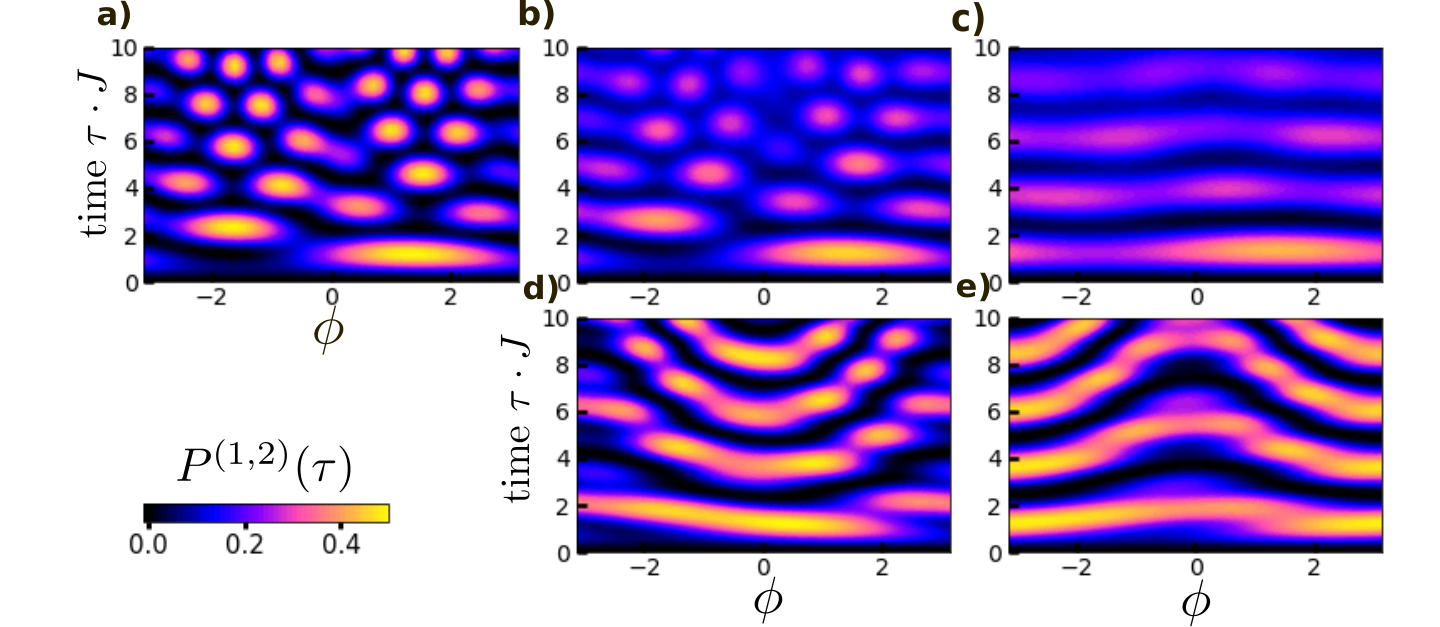
In Fig. 7 we investigate the waiting-time distribution $P^{(1,2)}(t)$ as a function of $\phi$ for different parameters. In Fig. 7(a) we consider the case $\gamma=0$, which exhibits an interesting pattern that breaks the $\phi\leftrightarrow-\phi$ symmetry. In particular, for $\phi>0$ the waiting time distribution reaches faster a maximum than for a negative $\phi$. This is in agreement with the explanations of Fig. 6.

Figures 7(b) and (c) depict the influence of dephasing on the waiting time statistics. In Fig. 7(b), we consider an intermediate dephasing parameter $\gamma=1$ and observe that the pattern is essentially equivalent to Fig. 7(a), but more smeared by decoherence.

The observations in Fig. 7(c), where we consider a strong system-bath coupling $\gamma=5$, is remarkable. Although the $\phi$ dependence has almost vanished for large times $\tau\cdot J>4$, the $\phi$ dependence is still clearly pronounced for short times. Here, the influence of the heat bath $n=3$ onto the dynamics becomes particular obvious. A positive $\phi$ directs the particle from site $n=1$ to $n=2$ at short times, so that the short-time waiting-time distribution is reminiscence to the $\gamma=0$ case. A negative $\phi$ directs the particle to the dephasing site $n=3$, so that the action of the dephasing is visible even at short times.

In Fig. 7(d) and (e) we investigate the influence of the onsite potential $\epsilon^{\prime}_{3}$ by considering $\epsilon^{\prime}_{3}=J$ and $\epsilon^{\prime}_{3}=7J$ for $\gamma=0$. Although the waiting time distribution is still sensitive on the phase, the broken symmetry $\phi\leftrightarrow-\phi$ is less obvious then in Fig. 7(a). This is a consequence of the large detuning of $\epsilon^{\prime}_{3}$ in comparison to $\epsilon_{1}=3J$ and $\epsilon_{2}=4J$, which makes the transfer over $n=3$ unlikely. Thus, the ring structure, an essential ingredient for the AB effect, is weakened. As a consequence, the isolated probability maxima observed in Fig. 7(a) become horizontally extended and connected, so that they form a band-like pattern as we can see clearly in Fig. 7(d). This resembles the decreased dependence on $\phi$. A similar pattern can be found in 7(e), at which the bands are more deformed.

To analytically evaluate the interference effect, we distribute the dynamics of the charge into the two path ways which the particle can take as shown in the sketches of Fig. 6. The probability that the charge is located on site $n=2$ at time $t$ with the initial population at $n=1$ at time $t=0$ is given by

where the time evolution operator $\hat{U}(t)$ of the system is approximated by a sum of two time evolution operators $\hat{U}^{(0)}$ and $\hat{U}^{(1)}$. These two operators are related to $\hat{U}(t)$ by replacing either $J_{3}=J_{2}\rightarrow 0$ or $J_{1}\rightarrow 0$, respectively.

For simplicity, we assume here that $\epsilon_{n}=\epsilon$, and $J_{n}=J$. The calculation of the right hand site of Eq. (23) can be performed analytically as shown in Appendix D. We find

This expression allows for an intuitive interpretation of the interference pattern observed in Fig. 7(a)-(c). We find a maximum constructive interference for $\phi=\frac{\pi}{2}$, while for $\phi=-\frac{\pi}{2}$ we observe a destructive interference for short times. Moreover, for $\phi=\frac{\pi}{2}$ the amplitude is maximal at $J\cdot t\approx\frac{\pi}{2}$, while for $\phi=-\frac{\pi}{2}$ it is maximal for $J\cdot t\approx 3\frac{\pi}{2}$. Although we have assumed that $\epsilon_{n}$ are all equal, this is in good agreement with the observation in Fig. 7(a)-(c).

However, this approach fails to describe the pattern in Fig. 7(d)-(e). In the approximation Eq. (23), we have assumed that both paths are equally likely. If $\epsilon^{\prime}_{3}$ is detuned from $\epsilon_{1}$ and $\epsilon_{2}$, then the charge will prefer the direct way $1\rightarrow 2$, as this constitutes a resonant particle transfer. This preference is not incorporated in Eq. (23).

Figures 7 (a)-(c) shed new light on the dynamics of the three-site model. Let us compare two observations. First, right after the charge is localized at $t=t_{0}$, its dynamics is sensitive to $\phi$ and evolves according to the system Hamiltonian and thus the AB effect, as can be seen in all panels in Fig. 7. Second, the dephasing does not occur immediately, but the phase information becomes gradually deleted and vanishes at long times $\tau\cdot J\approx 4$ in Fig. 7 (c). Thus, in contrast to the rapid onset of the AB effect, the dephasing is a cumulative effect. In particular, observing Fig. 7(c), we conclude that the dephasing takes place only when the particle passes site $n=3$. Our findings are consistent with Ref. [63], which demonstrated that in transport through molecules with localized dephasing probe decoherence does not take place immediately.

In Fig. 8, we investigate the impact of dephasing onto the system in more detail. In Fig. 8(a) we depict the dependence of $\kappa$ on the system-bath coupling $\gamma$. The exponential decrease according to Eq. (8) is determined by the temperature $T_{3}$. For $\gamma=5$ as in Fig. 7(c), we find a reduction of $50\%$, so that the ring structure is still quite strong. In Fig. 8(b)-(d), we investigate the transition rate $g_{\mu\nu}$ determining the thermally induced transitions between eigenstates $\mu$ to $\nu$ in the Redfield equation (10). For the rate $g_{12}$ at $\phi=\pi$ we find a crossover from an increasing rates for small $\gamma$ to a decreasing rate at large $\gamma$. The maximum can be found around $\gamma=3$. This is a typical feature for the crossover from week to strong coupling [11, 46]. It is surprising to see in Fig. 8(b) that $g_{12}$ strongly depends on $\phi$ for $\gamma=3$. While it is maximal at $\phi=\pi$, it is minimal for $\phi=0$. In contrast, $g_{23}$ exhibits a complementary behavior.

The rates can be written as a product $g_{\mu\nu}=C(E_{\mu}-E_{\nu})\cdot A_{\mu\nu}$, where $C(x)$ denotes the bath correlation function which depends on the energy differences and $A_{\mu\nu}$ depends on the coupling operators Eq. (9) and the eigenstate wave function of the polaron-transformed system Hamiltonian. Considering the spectra for small and large $\gamma$ in Fig. 3(a), we find that the spectral dependence on $\phi$ reduces for larger $\gamma$, as $\kappa$ decreases. Thus, we can infer that the strong $\phi$ dependence observed in Fig. 8 is caused by the wave function deformation. The rate of $g_{13}$ is relatively small compared to the other rates as the thermal activation energy $E_{3}-E_{1}$ is relatively large.

References

- [1] A. Bohm, A. Mostafazadeh, H. Koizumi, Q. Niu, and J. Zwanziger, The geometric phase in quantum systems (Springer Verlag Berlin Heidelberg, 2003).
- [2] R. G. Chambers, Phys. Rev. Lett. 5, 3 (1960).
- [3] N. Osakabe, T. Matsuda, T. Kawasaki, J. Endo, A. Tonomura, S. Yano, and H. Yamada, Phys. Rev. A 34, 815 (1986).
- [4] A. Van Oudenaarden, M. H. Devoret, Y. V. Nazarov, and J. E. Mooij, Nature 391, 768 (1998).
- [5] R. A. Webb, S. Washburn, C. P. Umbach, and R. B. Laibowitz, Phys. Rev. Lett. 54, 2696 (1985).
- [6] A. Bachtold, C. Strunk, J. Salvetat, J. Bonard, L. Forro, T. Nussbaumer, and C. Schonenberger, Nature 397, 673 (1999).
- [7] A. Aharony, S. Takada, O. Entin-Wohlman, M. Yamamoto, and S. Tarucha, New Journal of Physics 16, 083015 (2014).
- [8] A. Aharony, Y. Tokura, G. Z. Cohen, O. Entin-Wohlman, and S. Katsumoto, Phys. Rev. B 84, 035323 (2011).
- [9] M. W.-Y. Tu, W.-M. Zhang, J. Jin, O. Entin-Wohlman, and A. Aharony, Phys. Rev. B 86, 115453 (2012).
- [10] B. Liu, Y. Li, J. Zhou, T. Nakayama, and B. Li, Physica E: Low-dimensional Systems and Nanostructures 80, 163 (2016).
- [11] C. Wang, J. Ren, and J. Cao, New Journal of Physics 16, 045019 (2014).
- [12] R. Silbey and R. A. Harris, Journal of Chemical Physics 80, 2615 (1984).
- [13] R. A. Harris and R. Silbey, Journal of Chemical Physics 83, 1069 (1985).
- [14] M. O. Scully and M. Fleischhauer, Phys. Rev. Lett. 69, 1360 (1992).
- [15] M. O. Scully, Phys. Rev. Lett. 67, 1855 (1991).
- [16] C. Pöltl, C. Emary, and T. Brandes, Phys. Rev. B 87, 045416 (2013).
- [17] C. Emary, Phys. Rev. B 76, 245319 (2007).
- [18] C. Flindt, C. Fricke, F. Hohls, T. Novotnỳ, K. Netočnỳ, T. Brandes, and R. J. Haug, Proc. Natl. Acad. Sci. USA 106, 10116 (2009).
- [19] T. Wagner, P. Strasberg, J. C. Bayer, E. P. Rugeramigabo, T. Brandes, and R. J. Haug, Nat. Nanotechnol. 12, 218 (2017).
- [20] D. V. Averin, M. Möttönen, and J. P. Pekola, Phys. Rev. B 84, 245448 (2011).
- [21] P. A. Camati, J. P. S. Peterson, T. B. Batalhão, K. Micadei, A. M. Souza, R. S. Sarthour, I. S. Oliveira, and R. M. Serra, Phys. Rev. Lett. 117, 240502 (2016).
- [22] L. Gaudreau, S. A. Studenikin, A. S. Sachrajda, P. Zawadzki, A. Kam, J. Lapointe, M. Korkusinski, and P. Hawrylak, Phys. Rev. Lett. 97, 036807 (2006).
- [23] M. C. Rogge and R. J. Haug, Phys. Rev. B 77, 193306 (2008).
- [24] T. Fujisawa, T. Hayashi, R. Tomita, and Y. Hirayama, Science 312, 163 (2006).
- [25] K. Kobayashi, H. Aikawa, S. Katsumoto, and Y. Iye, Journal of the Physical Society of Japan 71, 2094 (2002).
- [26] E. Strambini, V. Piazza, G. Biasiol, L. Sorba, and F. Beltram, Phys. Rev. B 79, 195443 (2009).
- [27] S. V. Aradhya and L. Venkataraman, Nature nanotechnology 8, 399 (2013).
- [28] N. Tao, Nature nanotechnology 1, 173 (2006).
- [29] A. Nitzan and M. A. Ratner, Science 300, 1384 (2003).
- [30] N. A. Zimbovskaya, Transport Properties of Molecular Junctions (Springer New York, 2013).
- [31] D. Xiang, X. Wang, C. Jia, T. Lee, and X. Guo, Chemical Reviews 116, 4318 (2016).
- [32] J.-H. Jiang, M. Kulkarni, D. Segal, and Y. Imry, Phys. Rev. B 92, 045309 (2015).
- [33] D. Secker, S. Wagner, S. Ballmann, R. Härtle, M. Thoss, and H. B. Weber, Phys. Rev. Lett. 106, 136807 (2011).
- [34] O. Tal, M. Krieger, B. Leerink, and J. M. van Ruitenbeek, Phys. Rev. Lett. 100, 196804 (2008).
- [35] N. Neel, J. Kroger, and R. Berndt, Nano Letters 11, 3593 (2011).
- [36] D. Djukic and J. M. Van Ruitenbeek, Nano Letters 6, 789 (2006).
- [37] M. Tsutsui, M. Taniguchi, and T. Kawai, Nature Communications 1, 138 (2010).
- [38] C. M. Guédon, H. Valkenier, T. Markussen, K. S. Thygesen, J. C. Hummelen, and S. J. van der Molen, Nature Nanotechnology 7, 305 (2012).
- [39] H. Vazquez, R. Skouta, S. Schneebeli, M. Kamenetska, R. Breslow, L. Venkataraman, and M. Hybertsen, Nature Nanotechnology 7, 663 (2012).
- [40] M. Aidelsburger, M. Atala, M. Lohse, J. T. Barreiro, B. Paredes, and I. Bloch, Phys. Rev. Lett. 111, 185301 (2013).
- [41] G. Jotzu, M. Messer, R. Desbuquois, M. Lebrat, T. Uehlinger, D. Greif, and T. Esslinger, Nature (London) 515, 237 (2014).
- [42] B. A. Bernevig and T. L. Hughes, Topological Insulators and Topological Superconductors (Princeton University Press, 2013).
- [43] M. Fleischhauer and M. D. Lukin, Phys. Rev. A 65, 022314 (2002).
- [44] K.-J. Boller, A. Imamoğlu, and S. E. Harris, Phys. Rev. Lett. 66, 2593 (1991).
- [45] M. D. Lukin, M. Fleischhauer, A. S. Zibrov, H. G. Robinson, V. L. Velichansky, L. Hollberg, and M. O. Scully, Phys. Rev. Lett. 79, 2959 (1997).
- [46] C. Wang, J. Ren, and J. Cao, Scientific reports 5, 11787 (2015).
- [47] D. Xu and J. Cao, Frontiers of Physics 11, 110308 (2016).
- [48] D. Xu, C. Wang, Y. Zhao, and J. Cao, New Journal of Physics 18, 023003 (2016).
- [49] G. Schaller, Open quantum systems far from equilibrium, Vol. 881 (Springer, 2014).
- [50] S. Gurvitz, Frontiers of Physics 12, 120303 (2016).
- [51] O. Entin-Wohlman, A. Aharony, and Y. Imry, “Mesoscopic aharonov-bohm interferometers: Decoherence and thermoelectric transport,” in In Memory of Akira Tonomura, pp. 86–101.
- [52] D. Marcos, C. Emary, T. Brandes, and R. Aguado, New Journal of Physics 12, 123009 (2010).
- [53] J. Liu, C.-Y. Hsieh, and J. Cao, J. Chem. Phys. 148, 234104 (2018).
- [54] G. Engelhardt, M. Benito, G. Platero, G. Schaller, and T. Brandes, Phys. Rev. B 96, 241404 (2017).
- [55] T. Brandes, Ann. Phys. (Berlin) 17, 477 (2008).
- [56] D. S. Kosov, The Journal of Chemical Physics 146, 074102 (2017).
- [57] J. Thingna, D. Manzano, and J. Cao, Scientific reports 6, 28027 (2016).
- [58] J. Cao and R. J. Silbey, J. Phys. Chem. A 113, 13825 (2009).
- [59] P. Kwiat, H. Weinfurter, T. Herzog, A. Zeilinger, and M. A. Kasevich, Phys. Rev. Lett. 74, 4763 (1995).
- [60] L. Chirolli, E. Strambini, V. Giovannetti, F. Taddei, V. Piazza, R. Fazio, F. Beltram, and G. Burkard, Phys. Rev. B 82, 045403 (2010).
- [61] E. Strambini, L. Chirolli, V. Giovannetti, F. Taddei, R. Fazio, V. Piazza, and F. Beltram, Phys. Rev. Lett. 104, 170403 (2010).
- [62] National High Magnetic Field Laboratory Magnet Projects Page: https://nationalmaglab.org/magnet-development/magnet-science-technology.
- [63] S. Chen, Y. Zhang, S. Koo, H. Tian, C. Yam, G. Chen, and M. A. Ratner, Journal of Physical Chemistry Letters 5, 2748 (2014).
- [64] C. K. Lee, J. Moix, and J. Cao, The Journal of chemical physics 142, 164103 (2015).
Appendix A Polaron transformation
A.1 General Hamiltonian
A generalization of the Hamiltonian in Eq. (1) reads