Robust classification via MOM minimization
Abstract
We present an extension of Vapnik’s classical empirical risk minimizer (ERM) where the empirical risk is replaced by a median-of-means (MOM) estimator, the new estimators are called MOM minimizers. While ERM is sensitive to corruption of the dataset for many classical loss functions used in classification, we show that MOM minimizers behave well in theory, in the sense that it achieves Vapnik’s (slow) rates of convergence under weak assumptions: data are only required to have a finite second moment and some outliers may also have corrupted the dataset.
We propose an algorithm inspired by MOM minimizers. These algorithms can be analyzed using arguments quite similar to those used for Stochastic Block Gradient descent. As a proof of concept, we show how to modify a proof of consistency for a descent algorithm to prove consistency of its MOM version. As MOM algorithms perform a smart subsampling, our procedure can also help to reduce substantially time computations and memory ressources when applied to non linear algorithms. These empirical performances are illustrated on both simulated and real datasets.
1 Introduction
Machine learning has experienced unprecedented growth in recent years with a major societal impact exceeding that it has had in science for several decades. The article is set within the framework of robust learning theory, in the sense that only moment hypotheses are guaranteed on the data and the dataset may contain outliers. Robust learning theory has received particular attention in recent years, the aim sometimes being to construct reliable procedures under weaker assumptions than strong stochastic ones (such as the Gaussian character of noise in regression) and sometimes to detect outliers. This interest can be appreciated, for example, by the challenges recently posted on “kaggle”, the most popular data science competition platform. The 1.5 million dollars problem “Passenger Screening Algorithm Challenge” involves the discovery of terrorist activity from 3D images. The “NIPS 2017: Defense Against Adversarial Attack” consists in building algorithms robust to adversarial data.
Our approach extends Vapnik’s empirical risk minimization (ERM) (cf., [66]). The ERM is defined as a minimizer of the empirical risk over a class of functions from to :
| (1) |
where if and otherwise. This estimator is fairly insensitive to both heavy-tailed data and to the presence of a small proportion of outliers in the dataset (see Theorem 1 below). The reason is that the loss is bounded, which grants concentration no matter the distribution of and a small number of data cannot really impact the empirical mean performance. However, in practice, we find that algorithms supposed to approach ERM (usually following a convex relaxation principle) have poor performance in the presence of a few outliers. Figure 1 illustrates this problem on a toy example on which most of the data would be well separated by a linear classifier like Perceptron [61] or logistic classifier, but adding some anomalies completely flaws these algorithms.

The example in Figure 1 is representative of a general problem. Algorithms approaching ERM do not directly solve the minimization problem (1), which is NP-hard even for simple function classes like half-spaces indicators [26, 23]. Instead, the algorithm seeks to approach a convex relaxation of the problem, in which the considered loss (e.g. hinge or logistic loss) is not necessarily bounded. The advantage of this relaxation is that the function to be minimized is convex and that the minimum can easily be approached using for example gradient descent algorithms. On the other hand, this function becomes unbounded and can be diverted by a single outlier. Minimizing this corrupted criterion then leads to a bad classifier choice.
In learning theory, most alternatives to ERM manage the problem of outliers and heavy tail distributions for outputs only. These solutions are based on the pioneering work of John Tukey [64, 65], Peter Huber [32, 33] and Frank Hampel [27, 28], replacing the square loss by a robust alternative like Huber loss or Tuckey’s biweight loss. These methods do not allow to treat the case where the inputs are with heavy tails or corrupted, which is a classical problem in robust statistics also known as the “leverage point problem”, see [34]. In this article, we address this question by considering an alternative to M-estimators, called median-of-means. Several estimators based on this principle have recently been proposed in the literature [56, 42, 47, 48, 49, 53, 43]. To our knowledge, these articles use the small ball hypothesis [41, 54] to treat problems of least square regression or Lipschitzian loss regression. This assumption is restrictive in some classic functional regression frameworks [63, 29] or for problems such as the construction of recommendation system where inputs are sampled in the canonical basis and therefore do not satisfy a small ball condition. In this article, we propose a natural estimator based on the MOM principle, which we call MOM minimizer, and which we study without the small ball hypothesis. Instead we assume an a priori bound on the -norm of learning functions. We can identify mainly two streams of hypothesis in Learning theory: 1) boundedness with respect to some norm of the class of functions and the output , the typical example is the boundedness in assumption or 2) norm equivalence assumption over the class (or, more precisely, on the shifted class where is the oracle in ) and , the typical example being the subgaussian assumption, i.e. . The small ball assumption is a norm equivalence assumption between the and norms and is concerned with the second type of assumptions. Our approach deals with the first type of assumption since we only assume boundedness in which can be seen as an significant improvement upon a boundedness assumption even though the rates of convergence obtained for our estimators turn out to be minimax [18] in the absence of a margin condition [51] even under a assumption.
The estimation of the expectation of a univariate variable by median-of-means (MOM) [2, 37, 59] is done as follows: given a partition of the dataset into blocks of the same size, the empirical mean is constructed on each block and the MOM estimator is obtained by taking the median of these empirical means (see Section 2.2 for details). These estimators are naturally resistant to the presence of a few outliers in the dataset: if the number of these outliers does not exceed half the number of blocks, more than half of these blocks are made of “clean” data and the median is a reliable estimator.
In this article, we also study a family of algorithms approaching the MOM minimizer. The general idea we wish to promote is to use the MOM principle within algorithms originally intended for the evaluation of ERM associated to convex loss functions. In Section 4, we present the modification of gradient descent algorithms following this philosophy. The general principle of this iterative algorithm is as follows: at iteration , a dataset equipartition is selected uniformly at random and the most central block is determined according to the following formula
| (2) |
The next iteration is then produced by taking from a step down in the direction opposite to the gradient of at , cf. Algorithm 1. The underlying heuristic is that the data in the selected block are safe for estimating the mean at the point, in the sense that empirical risk is a subgaussian estimator of , cf. [19] and that data indexed by should not be outliers. The consistency of the algorithm is studied in Section 4.2. Theorem 3 provides an example showing how to modify the convergence proof of SGD algorithms.
In Section 5, the practical performances of this algorithm are illustrated on several simulations, involving in particular different loss functions. These simulations illustrate not surprisingly the gain of robustness that there is to use these algorithms in their MOM version rather than in their traditional version, as can for example be appreciated on the toy-example of Figure 1, cf. Figure 5. MOM estimators are compared to different learning algorithms on real datasets that can be modeled by heavy tailed data, obtaining in each case performances comparable to the best of these benchmarks.
Another advantage of our procedure is that it works on blocks of data. This can improve speed of execution and reduce memory requirements, which can be decisive on massive datasets and/or when one wishes to use non-linear algorithms as in Section 4.3. This principle of dividing the dataset to calculate estimators more quickly and then aggregating them is a powerful tool in statistics and machine learning [38]. Among others, one can mention bagging methods [12] or subagging —a variant of bagging where the bootstrap is replaced by subsampling— [15]. These methods are considered difficult to study theoretically in general and their analysis is often limited to obtaining asymptotic guarantees. By contrast, the theoretical tools for non-asymptotic risk analysis of MOM minimizer have already essentially been developed and the consistency of the algorithm can also be derived from standard arguments. Finally, subsampling by the central block ensures robustness properties that cannot be guaranteed by traditional alternatives.
The algorithm provides an empirical notion of data depth: data providing good risk estimates of are likely to be selected many times in the central block along the descent, while outliers will be systematically ignored. This notion of depth, based on the risk function, is very natural for prediction problems. It is complemented by an outliers detection procedure: data that are selected a number of times below a predetermined threshold are classified outliers. This procedure is evaluated on our toy example of Figure 1. Data represented by the dots in the top right corner all end with a null score (see Figure 9 below). The procedure is then tested on a real dataset on which the conclusions are more interesting. On this experiment, according to the theoretical bounds in Theorem 2, MOM minimizer’s prediction qualities are all the better when the number of blocks is small, cf. Figure 8. On the other hand, outlier detection is best when the number of blocks is large, cf. Figure 10. Outlier resistance and anomaly detection tasks can therefore both be handled using the MOM principle, but the main hyper-parameter – the number of blocks of data – for setting this method must be chosen carefully according to the objective. A number of blocks as small as possible (about twice the number of outliers) will give the best predictions, while large values of this number of blocks will accelerate the detection of anomalies. Note that it is essential for outliers detection to use different (for instance, random) partitions at each step of the descent to avoid giving the same score to an outlier and to all the data in the same block containing it.
Detecting outliers is usually performed in machine learning via some unsupervised preprocessing algorithm that detects outliers outside a bulk of data, see for example [35, 30, 17, 58] or other algorithms like DBSCAN [7] or isolation forest [46]. These algorithms assume elliptical symmetry of the data, a solution for skewed data can also be found in [36]. These unsupervised preprocessing removes outliers in advance, i.e. before starting any learning task. As expected, these strategies work well in the toy example from Figure 1. There are several cases where it will fail though. First, as explained in [34], this strategy classifies data independently of the risk, it is likely to remove from the dataset outlier coming from heavy-tailed distribution, yielding biased estimators. Moreover, a small group of misclassified data inside a bulk won’t be detected. Our notion of depth, based on the risk, seems more adapted to the learning task than any preprocessing procedure blind to the risk.
The paper is organized as follows. Section 2 presents the classification problem, the ERM and its MOM versions and gathers the assumptions granted for the main results. Section 3 presents theoretical risk bounds for the ERM and MOM minimizers on corrupted datasets. Section 4 deals with theoretical results on the algorithm computing MOM minimizers. We present the algorithm, study its convergence and provide theoretical bounds on its complexity. Section 5 shows empirical performance of our estimators in both simulated and real datasets. Proofs of the main results are postponed to Section 6 where we also added heuristics on the practical choice of the hyper-parameters.
2 Setting
2.1 Empirical risk minimization for binary classification
Consider the supervised binary classification problem, where one observes a sample , , taking values in . The set is a measurable space and . The goal is to build a classifier —that is, a measurable map — such that, for any new observation , is a good prediction for . For any classifier , let
The risk is a standard measure of the quality of a classifier. Following Vapnik [67], a popular way to build estimators is to replace the unknown measure in the definition of the risk by the empirical measure defined for any real valued function by and minimize the empirical risk. The empirical risk minimizer for the loss on a class of classifiers is .
The main issue with is that it cannot be computed efficiently in general. One source of computational complexity is that both and the loss function are non-convex. This is why various convex relaxations of the loss have been introduced since the very beginning of machine learning. These proceed in two steps. First, should be replaced by a convex set of functions taking values in . Then one builds an alternative loss function for defined for all . The new function should be convex and put less weight on those such that . Classical examples include the hinge loss , or the logistic loss . A couple such that is a convex set of real valued functions and is a convex function (i.e. for all and , is convex) such that whenever will be called a convex relaxation of . Given a convex relaxation of , one can define the associated empirical risk minimizer (ERM) by
| (3) |
Note that does not build a classifier. To deduce, a classification rule from one can simply consider its sign function defined for all by . The procedure is solution of a convex optimization problem that can therefore be approximated using a descent algorithm. We refer for example to [14] for a recent overview of this topic and Section 4 for more examples.
2.2 Corrupted datasets
In this paper, we consider a framework where the dataset may have been corrupted by outliers (or anomalies). There are several definitions of outliers in the literature, here, we assume that the dataset is divided into two parts. The first part is the set of inliers, indexed by , data are hereafter always assumed to be independent and identically distributed (i.i.d.) with common distribution . The second one is the set of outliers, indexed by which has cardinality . Nothing is assumed on these data which may not be independent, have distributions totally different from , with no moment at all, etc… In particular, this framework is sufficiently general to cover the case where outliers are i.i.d. with distribution as in the -contamination model [34, 16, 25, 21].
Our first result shows that the rate of convergence of is not affected by this corruption as long as does not exceed see Theorem 1 and the remark afterward. However, it is easy to remark that, when the number of data is finite as it is always the case in practice, even one aggressive outliers may yield disastrous breakdown of the empirical mean’s statistical performance. Consequently, even if behaves correctly, its proxy defined in (3) for a convex relaxation can have disastrous statistical performances, particularly when and are unbounded, cf. Figure 5 for an illustration.
To bypass this problem, we consider in this paper an alternative to the empirical mean called median-of-means [2, 37, 59]. Let denote an integer and let denote a partition of into bins of equal size . If doesn’t divide , one can always drop a few data. For any function and any non-empty subset , define the empirical mean on by . The median-of-means (MOM) estimator of is defined as the empirical median of the empirical means on the blocks
As the classical Huber’s estimator [32], MOM estimators interpolate between the unbiased but non robust empirical mean and the robust but biased median. In particular, when applied to loss functions, these new estimators of the risk suggest to define the following alternative to Vapnik’s ERM, called MOM minimizers
| (4) |
From a theoretical point of view, we will prove that, when the number of outliers is smaller than , performs well under -moments assumptions on and . To illustrate our main assumptions and theoretical results, we will regularly use the following classical example.
Example 1 (linear classification.).
Let and let denote the classical Euclidean norm on . Let denote a set of linear functions
Let denote either the hinge loss or the logistic loss defined respectively for any and by
2.3 Main assumptions
As already mentioned, data are divided into two groups, a subset made of outliers (on which we will make no assumption) and the remaining data contains all data that bring information on the target/oracle
Data indexed by are therefore called inliers or informative data. To keep the presentation as simple as possible, inliers are assumed to be i.i.d. distributed according to although this assumption could be relaxed as in [42, 43]. Finally, note that the partition of the dataset is of course unknown from the statistician.
Let us now turn to the set of assumptions we will use to study MOM minimizers procedures. For any measure and any function for which it makes sense, denote by . Denote also, for all , by the set of real valued functions such that and, for any , by
Our first assumption is an -assumption on the functions in .
Assumption 1.
For all , we have .
Of course, Assumption 1 is granted if is a set of classifiers. It also holds for the linear class of functions from Example 1 as long as with .
The second assumption deals with the complexity of the class . This complexity appears in the upper bound of the risk. It is defined using only informative data. Let
Definition 1.
Let denote a class of functions and let denote i.i.d. Rademacher random variables independent from . The Rademacher complexity of is defined by
The Rademacher complexity is a standard measure of complexity in classification problems [5]. It can be upper bounded, depending on the situation, by the VC dimension or the Dudley’s entropy integral or the Gaussian mean width of the class , see for example [9, 39, 5, 10, 18] for a presentation of these classical bounds. Our second assumption is simply that the Rademacher complexity of the class is finite.
Assumption 2.
The Rademacher complexity of is finite, .
Assumption 2 holds in the linear classification example under Assumption 1 since it follows from Cauchy-Schwarz inequality that . Finally, our last assumption is that the loss function considered is Lipschitz in the following sense.
Assumption 3.
The loss function satisfies for all and all ,
3 Theoretical guarantees
Our first result follows Vapnik’s original risk bound for the ERM and shows that is insensitive to the presence of outliers in the dataset. Moreover, it quantifies this robustness property since Vapnik’s rate of convergence is still achieved by when there are less than (number of observations) times (Vapnik’s rate of convergence) outliers.
Theorem 1.
Let denote a collection of classifiers. Let be the family of excess loss functions indexed by where . For all , with probability at least , we have
Theorem 1 is proved in Section 6.1. It is an adaptation of Vapnik’s proof of the excess risk bounds satisfied by in the presence of outliers.
Remark 1.
In the last result, one can easily bound the excess risk using instead of since
The final bound is of similar flavor: for all , with probability at least , we have
| (5) |
Remark 2.
When is the class of all linear classifiers, that is when , one has (see Theorem 3.4 in [9]). Therefore, when , Theorem 1 implies that for all , with probability at least ,
As a consequence, when the number of outliers is such that , Vapnik’s classical “slow” rate of convergence is still achieved by the ERM even if outliers have polluted the dataset. The interested reader can also check that “fast rates” could also be achieved by the ERM in the presence of outliers if and when the so-called strong margin assumption holds (see, [9, 9]). Note also that the previous remark also holds if is a class with VC dimension beyond the case of indicators of half spaces.
The conclusion of Theorem 1 can be misleading in practice. Indeed, theoretical performance of the ERM for the loss function are not downgraded by outliers, but its proxies based on convex relaxation of are. This can be seen on the toy example in Figure 1 and in Figure 5 from Section 5. In this work, we propose a robust surrogate, based on MOM estimators of the risk and defined in (2), to the natural empirical risk estimation of the risk which works for unbounded loss functions. In the next result, we prove that the MOM minimizer defined as
| (6) |
satisfies an excess risk bound under weak assumptions introduced in Section 2.
Theorem 2.
Theorem 2 is proved in Section 6.2. Compared to Theorem 1, achieves the same rate under the same conditions on the number of outliers with the same exponential control of the probability as for the ERM . The main difference is that the loss function may be unbounded, which is often the case in practice. Moreover, unlike classical analysis of ERM obtained by minimizing an empirical risk associated with a convex surrogate loss function, we only need a second moment assumption on the class .
These theoretical improvements have already been noticed in previous works [56, 20, 42, 47, 48, 49, 53, 43]. Contrary to tournaments of [49], Le Cam MOM estimators of [42] or minmax MOM estimators [43], Theorem 2 does not require the small ball assumption on but only shows “slow rates” of convergence. These slow rates are minimax optimal in the absence of a margin or Bernstein assumption [6, 51]. Proof of Theorem 2 does not enable fast rates to be obtained. Indeed, the non-linearity of the median excludes the possibility of using localization techniques leading to these fast rates. However, we show in the simulation study (cf. left side picture of Figure 14) that fast rates seem to be reached by the MOM minimizer.
The main advantage of our approach is its simplicity, we just have to replace empirical means by their MOM alternative in the definition of the ERM. Moreover, as expected, this simple alternative to ERM yields a systematically way to modify algorithms designed for approximating the ERM. The resulting “MOM version” of these algorithms are more robustness and faster than their original “ERM version”. Before illustrating these facts on simulations, let us describe algorithms approximating MOM minimizers.
4 Computation of MOM minimizers
In this section, we present first a generic algorithm to provide a MOM version of descent algorithms minimizing the empirical risk. We show how classical convergence proofs can be adapted to these algorithms.
4.1 MOM algorithms
The general idea is that any descent algorithms such as gradient descent, Newton method, alternate gradient descent, etc. (cf. [57, 14, 11, 4]) can easily be turned into a robust MOM-version. To illustrate this idea, a basic gradient descent is analyzed in the sequel.
The choice of blocks greatly influences the practical performance of the algorithm. In particular, a recurring flaw is that iterations tend to get stuck in local minima, which greatly slows the convergence of the alogorithm. To overcome this default and improve the stability of the procedure, we modify the partition at each iteration by drawing it uniformly at random, cf. step 2 of Algorithm 1.
Let denote the set of permutations of . For each , let denote an equipartition of defined for all by
To simplify the presentation, let us assume the class to be parametrized , for some . Let’s assume that the function is as regular as needed and convex (a typical example is for all ). Denote by the gradient or subgradient of in . The step-sizes sequence is denoted by and satisfies the classical conditions: and . Iterations will go on until a stopping time has been achieved. With these notations, a generic MOM version of a gradient descent algorithm (with random choice of blocks) is detailed in Algorithm 1.
Remark 3 (MOM gradient descent algorithm and stochastic block gradient descent).
Algorithm 1 can be seen as a stochastic block gradient descent (SBGD) algorithm minimizing the function using a given dataset. The main difference with the classical SBGD is that the choice of the block along which the gradient direction is performed is chosen according to a centrality measure computed thanks to the median operator in step 4 of Algorithm 1.
4.2 Convergence properties
We denote by the dataset. We consider the following set of assumptions:
Assumption 4.
There exist and a sequence of decreasing positive numbers , such that
- H-1
for all ,and -almost all , ,
- H-2
for almost all datasets , there exists a unique minimum where denotes the expectation with respect to , the uniformly distributed permutation used to construct the blocks of data,
- H-3
,
- H-4
,
- H-5
for almost all datasets , for Lebesgue almost all , for all ,
- H-6
for almost all datasets and Lebesgue almost all , there exists an open convex set containing such that for any equipartition of into blocks there exists such that for all , .
Recall that the dataset may contain outlier, which might be deterministic. We use the terminology “for almost all datasets such assumption holds” when the latter holds for -almost all informative data and for every outliers .
Theorem 3 (Convergence of the algorithm).
Note that Theorem 3 insures the convergence of the MOM version of the gradient descent algorithm with random blocks as defined in Algorithm 1 toward a minimizer of the conditional expectation . It does not prove its convergence toward a minimizer of the MOM criteria . Nevertheless, we can expect a strong concentration of around by concentration of random permutations, see [52].
Remark 4.
[MOM gradient descent, SGD and assumption H-6] All assumptions in Theorem 3 are the classical assumption used to prove the convergence of the classical SGD except for H-6 which is specific to MOM algorithms.
Indeed, the picture of the MOM gradient descent algorithm is pretty simple and depicted in Figure 2. At every step , the median operator makes a partition of into cells for – this partition changes at every step because the blocks are chosen randomly at the beginning of every step according to the random partition . We want every iteration of the MOM algorithm to be in the interior of a cell and not on a frontier in order to differentiate the objective function at . This is indeed the case under H-6, given that in that case, there is an open neighbor of such that for all , where the index of the block is common to every . Therefore, to differentiate the objective function at one just needs to differentiate at . The objective function to minimize is differentiable almost everywhere under H-6 and a gradient of the objective function is given by .
Remark 5 (Assumption H-5).
The assumption H-5 illustrate why we used a random shuffle of the data at each step of the algorithm, the principle is that the MOM risk in general may present local minima and hence the algorithm without the shuffle would stop in a local minimum. By using the random shuffle at each step, it seems that the problem has a unique minimum, at least experiment seems to say so. For example, in figure 3 we see the plot of the loss function when we change one of the parameters (the intercept) of a linear classifier for the classification problem depicted in figure 4.


Example 2.
Let us give a relatively general example where Assumption H-6 is satisfied. Let be an equipartition and let be defined for all by,
where for all blocks and the blocks are rearranged blocks defined such that . Proposition 1 shows that Assumption H-6 is satisfied in several situations.
Before stating the proposition, recall that the hazard function of an absolutely continuous real-valued random variable is defined for all by where is the density function of and is its cumulative distribution function.
Proposition 1.
Let be real-valued random variables and let be a family of functions with values in , if for all , the function is Lipshitz and the probability distribution of a mean of a block is a random variable (recall that the choice of block is random) with a bounded hazard function, then with probability , Assumption H-6 is satisfied, in particular, the partial derivative of with respect to the coordinate is given for almost all by
where denote the derivative with respect to the coordinate of .
Proposition 1 is proved in Section 6. The function is bounded for a large panel of probability distributions. For example, an exponential variable with parameter has a constant hazard function equal to ; a Cauchy random variable has also a bounded hazard function. Intuitively, this property of derivation of the median of means is more easily verified when the distribution of is heavy tailed (i.e. the mean blocks are far from one another) and in fact we can verify that the hazard function of the Gaussian is unbounded and hence this proposition cannot be used on Gaussian random variables.
4.3 Complexity of MOM risk minimization algorithms
Let be the computational complexity of a single ERM gradient descent update step on a dataset of size and let be the computational complexity of the evaluation of the loss function on a dataset containing data. Here the computational complexity is simply the number of basic operations needed to perform a task [3].
For each epoch, we begin by computing the “MOM empirical risk”. We perform times evaluations of the loss function, then we sort the means of these blocks of loss to finally get the median. The complexity of this step is then , assuming that the sort algorithm is in (like quick sort [31]). Then we do the ERM gradient step on a sample of size . Hence, the time complexity of this algorithm is
Example 3 (Linear complexity ERM algorithms).
For example, if the ERM gradient step and the loss function evaluation have linear complexity – like Perceptron or Logistic Regression – the complexity of the MOM algorithm is against for the ERM algorithm. Therefore, the two complexities are of the same order and the only advantage of MOM algorithms lies in their robustness to outliers.
Example 4 (Super-linear complexity ERM algorithms).
If on the other hand the complexity is more than linear as for Kernel Logistic Regression (KLR), taking into account the matrix multiplications whose complexity can be found in [24], the complexity of the MOM version of KLR, due to the additional need of the computation of the kernel matrix, is against for the ERM version. MOM versions of KLR are therefore faster than the classical version of KLR on top of being more robust. This advantage comes from the fact that MOM algorithms work on blocks of data instead on the entire dataset at every step. More informations about Kernel Logistic Regression can be found in [62] for example.
In this last example, the complexity comes in part from the evaluation of the kernel matrix that can be computationally expensive. Following the idea that MOM algorithms are performing ERM algorithm restricted to a wisely chosen block of data, then one can modify our generic strategy in this particular example to reduce drastically its complexity. The idea here is that we only need to construct the kernel matrix on the median block. The resulting algorithm, called Fast KLR MOM is described in Figure 2.
In Figure 2, we compute only the block kernel matrices, denoted by and constructed from the samples in the block . We also denote by the row in .
There are several drawbacks in the approach of Algorithm 2. First, the blocks are fixed at the beginning of the algorithm; therefore the algorithm needs a bigger dataset to work well and it may converge to a local minimum. Nonetheless, from the complexity point of view, this algorithm will be much faster than both the classical KLR and MOM KLR (see below for a computation of its complexity) which is important given the growing use of kernel methods on very large databases for example in biology. The choice of should ultimately realize a trade-off between complexity and performance (in term of accuracy for example) when dealing with big databases containing few outliers.
Example 5 (Complexity of Fast KLR-MOM algorithm).
The complexity of Fast KLR-MOM is against for the ERM version.
5 Implementation and Simulations
5.1 Basic results on a toy dataset
The toy model we consider models outliers due to human or machine errors we would like to ignore in our learning process. It is also a dataset corrupted to make linear classifiers fail. The dataset is a 2D dataset constituted of three “labeled Gaussian distribution”. Two informative Gaussians and with label respectively and and one outliers Gaussian with label . In other words, the distribution of informative data is given by , and . Outliers data have distribution given by a.s. and .

The algorithms we study are the MOM adaptations of Perceptron, Logistic Regression and Kernel Logistic Regression.
Based on our theoretical results, we know that the number of blocks has to be larger than times the number of outliers for our procedure to be on the safe side. The value is therefore used in all subsequent applications of MOM algorithms on the toy dataset except when told otherwise. To quantify performance, we compute the miss-classification error on a clean dataset made of data distributed like the informative data.
For Kernel Logistic Regression, we study here a linear kernel because outliers in this dataset are clearly adversarial when dealing with linear classifiers. The algorithm can also use more sophisticated kernels, a comparison of the MOM algorithms with similar ERM algorithms is represented in figure 5, the ERM algorithms are taken from the python library scikit-learn [60] with their default parameters.
Figure 5 illustrates resistance to outliers of MOM’s algorithms compared to their classical version.

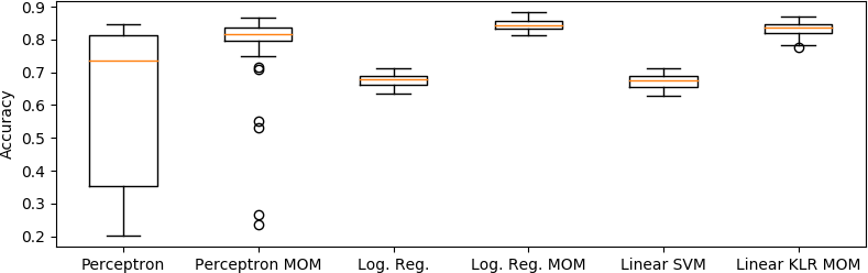
These first results are completed in Figure 6 where we computed accuracy on several run of the algorithms. These results confirm the visual impression of our first experiment.
Finally, we illustrate our results regarding complexities of the algorithms on a simulated example. MOM algorithms have been computed together with state-of-the art algorithms from scikit-learn [60] (we use Random forest, SVM classifier as well as SGD classifier optimizing Huber loss which entail a robustness in but not in , see [34, Chapter 7]) on a simulated dataset composed of two Gaussian blobs and with label respectively and . We sample points for the training dataset and for the test dataset. The parameters used in the algorithms are those for which we obtained the optimal accuracy, (this accuracy is illustrated in the next section). Time of training plus time of evaluation on the test dataset are gathered in Figure 7.
| Algorithm | Perceptron MOM | Log. Reg. MOM | KLR MOM | Fast KLR MOM |
|---|---|---|---|---|
| Time (s) | ||||
| Algorithm | Rand. Forest | SVM | SGD Hub. loss | |
| Time (s) |
Not surprisingly, very efficient versions of linear algorithms from Python’s library are extremely fast (results are sometimes provided before we even charged the dataset in some experiments). The performance of our algorithm are nevertheless acceptable in general (around 5 times longer than random forest for example). The important fact here is that non linear algorithms such as SVM take much more time to provide a result. FAST KLR MOM is able to reduce substantially the execution time of SVM with comparable predictive performance.
5.2 Applications on real datasets
We used the HTRU2 dataset, also studied in [50], that is provided by the UCI Machine Learning Repository. The goal is to detect pulsars (a rare type of Neutron star) based on radio emission detectable on earth from which features are extracted to gives us this dataset. The problem is that most of the signal comes from noise and not pulsar, the goal is then to classify pulsar against noise, using the points in the dataset.
The accuracy of different algorithms is obtained using on several runs of the algorithms each using 4/5 of the datasets for training and for testing algorithms. Boxplots presenting performance of various algorithms are displayed in Figure 8. To improve performance, RBF kernel was used both for KLR MOM and Fast KLR MOM.

5.3 Outlier detection with MOM algorithms
When we run MOM version of a descent algorithm, we select at each step a block of data points realizing the median of a set of “local/block empirical risk” at the current iteration of the algorithm. The number of times a point is selected by the algorithm can be used as a depth function measuring reliability of the data. Note that this definition of depth of a data point has the advantage of taking into account the learning task we want to solve, that is the loss and the class . It means that outliers are considered w.r.t. the problem we want to solve and not w.r.t. some a priori notion of centrality of points in unrelated with the problem considered at the beginning.
We apply this idea on the toy dataset with the Logistic Regression MOM algorithm. Results are gathered in a sorted histogram given in Figure 9. Red bars represent outliers in the original datasets.

Quite remarkably, outliers are in fact those data that have been used the smallest number of times. The method targets a very specific type of outliers, those disturbing the classification task at hand. If there was a point very far away from the bulk of data but in the half-space of its label, it wouldn’t be detected.
This detection algorithm doesn’t scale well when the dataset gets bigger as a large number of iterations is necessary to choose each point a fair number of times. For bigger datasets, we suggest to adapt usual outlier detection algorithms [1]. We emphasize that clustering techniques and K-Means are rather easy to adapt in a MOM algorithm and detect points far from the bulk of data. This technique might greatly improve usual K-Means as MOM K-Means is more robust.
Let us now analyze the effect of on the outlier detection task. The histogram of the smaller counts of points of HTRU2 dataset as gets bigger is plotted in Figure 10.

It appears from Figure 10 that measures the sensitivity of the algorithm. Severe outliers (as in the toy example) are detected for small while mild outliers are only discovered as gets bigger.
It seems therefore that the optimal choice of in MOM depends on the task one is interested in. For classification, should be as small as possible to get better risk bounds (but it still should be larger than the number of outliers) whereas for detecting outliers we may want to choose much larger to even detect an outlier, (but it should also be small enough for the underlying classification to perform correctly). As a proof of concept, for Pulsar database, we got optimal results choosing for classification whereas we only detect a significant amount of outliers when is around .
6 Proofs
6.1 Proof of Theorem 1
We adapt Vapnik’s classical analysis [66] of excess risk bound of ERM to a dataset corrupted by outliers. We first recall that and for all , the excess loss function of is . For simplicity we denote and for all , and .
It follows from the definition of the ERM that . Therefore, if we denote by (resp. ) the empirical measure supported on (resp. ), we have
because a.s.. Then, by the bounded difference inequality [10, Theorem 6.2], since all satisfies , one has, for any ,
Furthermore, by the symmetrization argument (cf. Chapter 4 in [45]),
Therefore, for any , with probability larger than ,
The proof is completed by choosing .
6.2 Proof of Theorem 2
Let . By definition, one has , therefore,
| (7) |
Let us now control the two expressions in the right-hand side of (7). Let . We have
where . Using Markov inequality together with , we obtain
when .
Now, for any , one has iff
| (8) |
Let us now control the probability that (8) holds via an adaptation of the small ball method [41, 55]. Let and let be defined for all . As , one has
where we recall that .
Since, and for all , , we have for all and ,
One has therefore
As , by the bounded-difference inequality, for any , with probability larger than ,
Now, by the symmetrization inequality,
Since is -Lipschitz and , by the contraction principle (see [45, Chapter 4] or more precisely equation (2.1) in [40]),
By the symmetrization principle,
Finally, since is -Lipschitz, by the contraction principle (see equation (2.1) in [40]),
6.3 Proof of Theorem 3
First, hypothesis H-6 implies that, for any , there exists an open convex neighbor of such that for all , . In particular therefore, for any ,
| (9) |
From here, the rest of the proof is identical to the proof of consistency of the SGD. As a proof of concept, we reproduce here the arguments of [8]. In what follows, all results are given conditionally on . We set
By definition of the update of the algorithm, we have
Let be the -algebra spanned by , we have
Then, we use Jensen’s inequality, we have
| (10) |
By convexity of , for any , we have
Therefore,
Hence, using hypothesis H-1 and H-5, we get
| (11) |
Now, defining and , it follows from (11) that
Using hypothesis H-3, we have that
From Doob’s first martingale convergence theorem (see for example [22, Theorem 5.2.8]), there exists such that
We plug this convergence in the inequality (10) to get
Then, using hypothesis H-3, we have
From the hypotheses H-4 and H-5, we can then conclude that
6.4 Proof of Proposition 1
We denote by the blocks such that the corresponding block empirical mean are sorted: . To simplify the notations we denote by that correspond to the rank of the median when is odd, we suppose odd.
Let us take , we show that for all with sufficiently small, we have for all .
To show that, it is sufficient to check that we have
We decompose this difference in three parts,
The two last terms are controlled by the Lipshitz property of ,
Then, we use order statistics and interquantile range to control the first term.
To do that, we use Renyi representation to say that the order statistics of the blocks can be expressed as functions of the order statistics of exponential variables. Let be K i.i.d sample with a standard Exponential law, then using the function where is the c.d.f of the random variable to make the link between the sample and the sample , we have
Then, because the hazard function is the inverse of the derivative of and is bounded by , we have by the mean value inequality,
hence, for all
which we can rewrite as: for all , with probability greater than ,
Finally, with probability greater than ,
Which implies that with probability greater than ,
Then, taking the union bound for , we have
We want to compute the partial derivatives of , to do that we denote by the canonical basis of and we define . We denote by the event
and we study the limiting event .
First, let us note that for all , the sequence of set is non-increasing, hence
then, for all , we can study the with Borel-Cantelli Lemma. Indeed, we have
Hence, the series converges and by Borel Cantelli Lemma, , then for all , .
Rewriting that we have that
Hence,
Hence,
which implies that for all , ,
7 Annex
7.1 Choice of the number of blocks
Let us study the behaviour of our algorithms when the number of blocks changes. We plot the accuracy as a function of averaged on 50 runs to have a good idea of the evolution of the performance with respect to , the result is represented in figure 11.

There is a clear separation around that is consistent with the theory. On the other hand the accuracy doesn’t decrease when gets bigger one would expect. This may be due to the symmetry of the dataset. If we run the same experiment on the real dataset, we get a much more regular plot, see Figure 12.

7.2 Illustration of convergence rate
In this section, we estimate the rate of convergence of the MOM risk minimization algorithm Logistic Regression on two databases (see figure 13). The first dataset is composed of points located on two interlaced half-circle with a Gaussian noise of standard deviation , the two ”moons” are each of a different class. We assume that these moons don’t satisfy the margin property (we checked that the rate was slow for ERM algorithms, using the vanilla logistic regression). The second dataset is composed of two Gaussians and with respective label and , we can prove that this dataset verifies the margin property needed to obtain fast rate in ERM


There are no outliers in the datasets because we only want to test the rate of convergence. To illustrate the rates of convergence of our algorithms, we plot the curve as a function of where the risk is estimated by Monte-Carlo. The figure obtained for Logistic Regression MOM is represented in figure 14. It seems that MOM minimizers can achieve fast rates of convergence even if we did not prove them.


Remark 6.
We used random blocks sampled at each iteration for this application because it is the algorithm that we described earlier but even if we use one partition of blocks for the whole algorithm (as in the theory we developed) we obtain nonetheless fast rate for the Gaussians dataset.
7.3 Comparison with robust algorithms based on M-estimators.
In this section we compare the algorithm Logistic Regression MOM with two other algorithms based on M-estimators, these algorithms are studied on the toy dataset presented in Section 5.
One algorithm is a gradient on the Huber estimation of the loss function, it follows the same reasoning as MOM risk minimization and minimizes using as a proxy the Huber estimator for this quantity. The Huber estimator is then defined as a -estimator, denoted here , solution of
where is the Huber function, . Using this definition of , it is then easy to compute the gradient and then use a gradient descent algorithm. The theory behind this algorithm is studied further in [13].
The second algorithm uses a ”redescending” loss function, in short we do ERM with a bounded loss function. Here we use Tukey biweight loss function rescaled by MADN scale estimator and IRLS algorithm to optimize the empirical risk.

Figure 15 shows that all algorithms perform similarly on this easy, low dimensional dataset. The situation is quite different in higher dimension. In Figure 16 we used a 200 dimensional dataset and the algorithm using a redescending loss function does not perform well. This may be due to local minima in which the algorithm gets stuck, as local minima are multiplied when the dimension gets higher. The other algorithms don’t suffer this drawback since they use a “projection by the loss function” that makes the problem one dimensional.

The algorithm using redescending loss functions is a simple gradient descent that has linear complexity. The Huber gradient algorithm estimates at each iteration a Huber estimator of location. The complexity of this estimator depends on the algorithm used but for most M-estimators a commonly used algorithm is an iteratively reweighted algorithm whose complexity is linear in the sample size. In practice we can nonetheless notice a great complexity of the Huber estimator in some cases where data are not well spread. In most cases, Logistic Regression MOM is the fastest among these three algorithms and the gradient Huber is the slowest, even though logistic regression may need a lot more iterations than the other algorithms.
References
- [1] Charu C. Aggarwal. Outlier Analysis. Springer Publishing Company, Incorporated, 2013.
- [2] Noga Alon, Yossi Matias, and Mario Szegedy. The space complexity of approximating the frequency moments. J. Comput. System Sci., 58(1, part 2):137–147, 1999. Twenty-eighth Annual ACM Symposium on the Theory of Computing (Philadelphia, PA, 1996).
- [3] Sanjeev Arora and Boaz Barak. Computational complexity. Cambridge University Press, Cambridge, 2009. A modern approach.
- [4] Francis Bach, Rodolphe Jenatton, Julien Mairal, and Guillaume Obozinski. Structured sparsity through convex optimization. Statist. Sci., 27(4):450–468, 2012.
- [5] Peter L. Bartlett and Shahar Mendelson. Rademacher and Gaussian complexities: risk bounds and structural results. J. Mach. Learn. Res., 3(Spec. Issue Comput. Learn. Theory):463–482, 2002.
- [6] Peter L. Bartlett and Shahar Mendelson. Empirical minimization. Probab. Theory Related Fields, 135(3):311–334, 2006.
- [7] Derya Birant and Alp Kut. St-dbscan: An algorithm for clustering spatial–temporal data. Data & Knowledge Engineering, 60(1):208–221, 2007.
- [8] Léon Bottou. On-line learning in neural networks. chapter On-line Learning and Stochastic Approximations, pages 9–42. Cambridge University Press, New York, NY, USA, 1998.
- [9] Stéphane Boucheron, Olivier Bousquet, and Gábor Lugosi. Theory of classification: a survey of some recent advances. ESAIM Probab. Stat., 9:323–375, 2005.
- [10] Stéphane Boucheron, Gábor Lugosi, and Pascal Massart. Concentration inequalities: A nonasymptotic theory of independence, 2013.
- [11] Stephen Boyd and Lieven Vandenberghe. Convex optimization. Cambridge University Press, Cambridge, 2004.
- [12] Leo Breiman. Bagging predictors. Machine Learning, 24(2):123–140, 1996.
- [13] Christian Brownlees, Emilien Joly, and Gábor Lugosi. Empirical risk minimization for heavy-tailed losses. Ann. Statist., 43(6):2507–2536, 12 2015.
- [14] S. Bubeck. Convex optimization: Algorithms and complexity. Foundations and Trends in Machine Learning, 8(3-4):231–357, 2015.
- [15] Peter Bühlmann and Bin Yu. Analyzing bagging. The Annals of Statistics, 30(4):927–961, 2002.
- [16] Mengjie Chen, Chao Gao, and Zhao Ren. Robust covariance and scatter matrix estimation under huber’s contamination model. Technical report, University of Chicago and University of Pittsburgh, 2017. Preprint available on arXiv:1506.00691.
- [17] Christophe CROUX and Catherine DEHON. Robust linear discriminant analysis using s-estimators. The Canadian Journal of Statistics / La Revue Canadienne de Statistique, 29(3):473–493, 2001.
- [18] Luc Devroye, László Györfi, and Gábor Lugosi. A Probabilistic Theory of Pattern Recognition, volume 31 of Applications of Mathematics. Springer, corrected 2nd edition, 1997. missing.
- [19] Luc Devroye, Matthieu Lerasle, Gabor Lugosi, and Roberto I. Oliveira. Sub-Gaussian mean estimators. Ann. Statist., 44(6):2695–2725, 2016.
- [20] Luc Devroye, Matthieu Lerasle, Gabor Lugosi, and Roberto I. Oliveira. Sub-gaussian mean estimators. The Annals of Statistics, 44(6):2695–2725, 2016.
- [21] D. Donoho and A. Montanari. Variance breakdown of huber (m)-estimators: . Technical report, Stanford University, 2015. Preprint available on arXiv:1503.02106.
- [22] Rick Durrett. Probability: Theory and examples, 2011.
- [23] Vitaly Feldman, Venkatesan Guruswami, Prasad Raghavendra, and Yi Wu. Agnostic learning of monomials by halfspaces is hard. SIAM J. Comput., 41(6):1558–1590, 2012.
- [24] François Le Gall. Powers of tensors and fast matrix multiplication. CoRR, abs/1401.7714, 2014.
- [25] Chao Gao. Robust regression via mutivariate regression depth. Technical report, University of Chicago, 2017. Preprint available on arXiv:1702.04656.
- [26] Venkatesan Guruswami and Prasad Raghavendra. Hardness of learning halfspaces with noise. SIAM J. Comput., 39(2):742–765, 2009.
- [27] Frank R Hampel. A general qualitative definition of robustness. The Annals of Mathematical Statistics, pages 1887–1896, 1971.
- [28] Frank R Hampel. The influence curve and its role in robust estimation. Journal of the American Statistical Association, 69(346):383–393, 1974.
- [29] Qiyang Han and Jon A. Wellner. A sharp multiplier inequality with applications to heavy-tailed regression problems. arXiv:1706.02410, 2017.
- [30] Xuming He and Wing K Fung. High breakdown estimation for multiple populations with applications to discriminant analysis. Journal of Multivariate Analysis, 72(2):151 – 162, 2000.
- [31] Charles AR Hoare. Quicksort. The Computer Journal, 5(1):10–16, 1962.
- [32] Peter J. Huber. Robust estimation of a location parameter. Ann. Math. Statist., 35:73–101, 1964.
- [33] Peter J Huber. The behavior of maximum likelihood estimates under nonstandard conditions. In Proceedings of the fifth Berkeley symposium on mathematical statistics and probability, volume 1, pages 221–233. Berkeley, CA, 1967.
- [34] Peter J Huber and Elvezio M Ronchetti. Robust statistics; 2nd ed. Wiley Series in Probability and Statistics. Wiley, Hoboken, NJ, 2009.
- [35] Mia Hubert and Katrien Van Driessen. Fast and robust discriminant analysis. Computational Statistics & Data Analysis, 45(2):301 – 320, 2004.
- [36] Mia Hubert and Stephan Van Der Veeken. Robust classification for skewed data. Adv. Data Anal. Classif., 4(4):239–254, December 2010.
- [37] Mark R. Jerrum, Leslie G. Valiant, and Vijay V. Vazirani. Random generation of combinatorial structures from a uniform distribution. Theoret. Comput. Sci., 43(2-3):169–188, 1986.
- [38] Michael I. Jordan. On statistics, computation and scalability. Bernoulli, 19(4):1378–1390, 2013.
- [39] Vladimir Koltchinskii. Oracle inequalities in empirical risk minimization and sparse recovery problems, volume 2033 of Lecture Notes in Mathematics. Springer, Heidelberg, 2011. Lectures from the 38th Probability Summer School held in Saint-Flour, 2008, École d’Été de Probabilités de Saint-Flour. [Saint-Flour Probability Summer School].
- [40] Vladimir Koltchinskii. Oracle inequalities in empirical risk minimization and sparse recovery problems. 2011.
- [41] Vladimir Koltchinskii and Shahar Mendelson. Bounding the smallest singular value of a random matrix without concentration. Int. Math. Res. Not. IMRN, (23):12991–13008, 2015.
- [42] G. Lecué and M. Lerasle. Learning from mom’s principle : Le cam’s approach. Technical report, CNRS, ENSAE, Paris-sud. Preprint available on arXiv:1701.01961.
- [43] G. Lecué and M. Lerasle. Robust machine learning by median-of-means : theory and practice. Technical report, CNRS, ENSAE, Paris-sud. Preprint available on arXiv:1711.10306.
- [44] Guillaume Lecué and Shahar Mendelson. Learning subgaussian classes: Upper and minimax bounds. Technical report, CNRS, Ecole polytechnique and Technion, 2013.
- [45] Michel Ledoux and Michel Talagrand. Probability in Banach spaces. Classics in Mathematics. Springer-Verlag, Berlin, 2011. Isoperimetry and processes, Reprint of the 1991 edition.
- [46] Fei Tony Liu, Kai Ming Ting, and Zhi-Hua Zhou. Isolation forest. In Data Mining, 2008. ICDM’08. Eighth IEEE International Conference on, pages 413–422. IEEE, 2008.
- [47] Gabor Lugosi and Shahar Mendelson. Regularization, sparse recovery, and median-of-means tournaments. Preprint available on arXiv:1701.04112.
- [48] Gabor Lugosi and Shahar Mendelson. Sub-gaussian estimators of the mean of a random vector. Preprint available on arXiv:1702.00482.
- [49] Gabor Lugosi and Shahar Mendelson. Risk minimization by median-of-means tournaments. Preprint available on ArXive:1608.00757, 2017.
- [50] R. J. Lyon, B. W. Stappers, S. Cooper, and J. D. Brooke, J. M. Knowles. Fifty Years of Pulsar Candidate Selection: From simple filters to a new principled real-time classification approach. MNRAS, 000:000–000, 2015.
- [51] Enno Mammen and Alexandre B. Tsybakov. Smooth discrimination analysis. Ann. Statist., 27(6):1808–1829, 1999.
- [52] COLIN McDIARMID. Concentration for independent permutations. Combinatorics, Probability and Computing, 11(2):163–178, 2002.
- [53] Shahar Mendelson. An optimal unrestricted learning procedure. Preprint available on arXiv:1707.05342.
- [54] Shahar Mendelson. Learning without concentration. In Proceedings of the 27th annual conference on Learning Theory COLT14, pages pp 25–39. 2014.
- [55] Shahar Mendelson. Learning without concentration. J. ACM, 62(3):Art. 21, 25, 2015.
- [56] Stanislav Minsker. Geometric median and robust estimation in Banach spaces. Bernoulli, 21(4):2308–2335, 2015.
- [57] Eric Moulines and Francis R Bach. Non-asymptotic analysis of stochastic approximation algorithms for machine learning. In Advances in Neural Information Processing Systems, pages 451–459, 2011.
- [58] Ernest Fokoue Necla Gunduz. Robust classification of high dimension low sample size data. 2015.
- [59] A. S. Nemirovsky and D. B. Yudin. Problem complexity and method efficiency in optimization. A Wiley-Interscience Publication. John Wiley & Sons, Inc., New York, 1983. Translated from the Russian and with a preface by E. R. Dawson, Wiley-Interscience Series in Discrete Mathematics.
- [60] F. Pedregosa, G. Varoquaux, A. Gramfort, V. Michel, B. Thirion, O. Grisel, M. Blondel, P. Prettenhofer, R. Weiss, V. Dubourg, J. Vanderplas, A. Passos, D. Cournapeau, M. Brucher, M. Perrot, and E. Duchesnay. Scikit-learn: Machine learning in Python. Journal of Machine Learning Research, 12:2825–2830, 2011.
- [61] Frank Rosenblatt. The perceptron: A theory of statistical separability in cognitive systems. Cornell Aeronautical Laboratory, Inc., Rep. No. VG-1196-G-1. U.S. Department of Commerce, Office of Technical Services, PB 151247, 1958.
- [62] Volker Roth. Probabilistic discriminative kernel classifiers for multi-class problems, 2001.
- [63] Adrien Saumard. On optimality of empirical risk minimization in linear aggregation. Bernoulli, 24(3):2176–2203, 2018.
- [64] John W Tukey. A survey of sampling from contaminated distributions. Contributions to probability and statistics, 2:448–485, 1960.
- [65] John W Tukey. The future of data analysis. The annals of mathematical statistics, 33(1):1–67, 1962.
- [66] Vladimir N. Vapnik. Statistical learning theory. Adaptive and Learning Systems for Signal Processing, Communications, and Control. John Wiley & Sons, Inc., New York, 1998. A Wiley-Interscience Publication.
- [67] Vladimir N. Vapnik. The nature of statistical learning theory. Statistics for Engineering and Information Science. Springer-Verlag, New York, second edition, 2000.