Log-Aesthetic Curves: Similarity Geometry,
Integrable Discretization and Variational Principles
Jun-ichi Inoguchi
Institute of Mathematics, University of Tsukuba
Tsukuba 305-8571, Japan
e-mail: inoguchi@math.tsukuba.ac.jp
Yoshiki Jikumaru
Institute of Mathematics for Industry, Kyushu University
744 Motooka, Fukuoka 819-0395, Japan
e-mail: y-jikumaru@imi.kyushu-u.ac.jp
Kenji Kajiwara
Institute of Mathematics for Industry, Kyushu University
744 Motooka, Fukuoka 819-0395, Japan
e-mail: kaji@imi.kyushu-u.ac.jp
Kenjiro T. Miura
Graduate School of Science and Technology, Shizuoka University
3-5-1 Johoku, Hamamatsu, Shizuoka, 432-8561, Japan
e-mail: miura.kenjiro@shizuoka.ac.jp
Wolfgang K. Schief
School of Mathematics and Statistics, The University of New South Wales
Sydney, NSW 2052, Australia
e-mail: w.schief@unsw.edu.au
Abstract
In this paper, we consider a class of plane curves called log-aesthetic curves and their generalization which are used in computer aided geometric design. We consider these curves in the framework of the similarity geometry and characterize them as invariant curves under the integrable flow on plane curves which is governed by the Burgers equation. We propose a variational principle for these curves, leading to the stationary Burgers equation as the Euler-Lagrange equation. As an application of the formulation developed here, we propose a discretization of these curves and the associated variational principle which preserves the underlying integrable structure. We finally present algorithms for the generation of discrete log-aesthetic curves for given data based on the similarity geometry. Our method is able to generate -shaped discrete curves with an inflection as well as -shaped curves according to the boundary condition. The resulting discrete curves are regarded as self-adaptive discretization and thus high-quality even with a small number of points.
1 Introduction
In this paper, we consider a class of plane curves in computer aided geometric design called the log-aesthetic curves (LAC) and their generalization called the quasi aesthetic curves (qAC), and present a new mathematical characterization based on the theory of integrable systems and similarity geometry. We then construct the discrete analogue of LAC and qAC within the above-mentioned framework, which gives a new implementation of LAC and qAC with a sound mathematical background as discrete curves.
In the previous paper [7], we have announced the similarity geometric framework of the LAC and the qAC, where these curves have been characterized as the invariant curves under the integrable flow on the plane curves preserving the similarity arc length. More precisely, the evolution of the curves is governed by the similarity curvature which is characterized by the stationary solutions of integrable nonlinear partial differential equation arising from the geometric setting. In addition, we have introduced a fairing energy functional and formulated the LAC and the qAC in terms of a variational principle. Here, we first present a detailed account of those results.
Secondly, we construct a discrete analogue of the LAC and the qAC based on the above formulation, where these curves are characterized as the invariant discrete curves under the discrete integrable flow on discrete plane curves preserving the similarity arc length. We then introduce a discrete fairing functional and formulate these discrete curves in terms of a discrete variational principle. The discrete curves obtained in this manner are not naïve approximations of the original LAC and qAC but admit their own natural geometric characterization.
Finally, we give an implementation of generation method of the discrete LAC obtained above for given endpoints and associated tangent vectors. We consider the cases of the discrete LAC without/with an inflection (“-shaped” / “-shaped”). We note that the discrete LAC based on the similarity geometry gives a kind of self-adaptive mesh discretization of the LAC, since we have dense points where the curvature is large and coarse points where the curvature is small.
2 Log-aesthetic curves and similarity geometry
Originally, LAC has been studied in the framework of Euclidean geometry. Before proceeding to LAC, we give a brief account of the treatment of plane curves in Euclidean geometry. Let be an arc length parametrized plane curve and be arc length. We introduce the Frenet frame by
| (1) |
where and are the tangent and the normal vector fields, respectively, and is the positive -rotation. Since by definition of arc length, we may write , where is called the angle function. The Frenet frame satisfies the Frenet formula
| (2) |
where is the curvature. Note that the curvature is related to the signed radius of curvature and the angle function by
| (3) |
According to [10], an arc length parametrized plane curve is said to be a LAC of slope if its signed curvature radius satisfies
| (4) |
Originally, LAC is characterized as a family of arc length parametrized curves whose logarithmic curvature histogram, a graph of versus , is a line, and is its slope [2, 3].
The class of LAC includes some well known plane curves. For instance, the logarithmic spiral, the clothoid, the Nielsen spiral are included as LAC of slope , , and , respectively. The LAC of slope is also known as the circle involute curve. These examples are illustrated in Figure 1.
LAC are now maturing in industrial and graphics design practices. Figure 2 shows the practical example of a car designed using LA splines. Figure 2(a) shows free-form surface iso-parametric lines generated using LA splines and corresponding zebra maps. Figure 2(b) shows the geometric model with a special lighting condition and 2(c) are photos of a manufactured mockup based on the geometric model. Note that the roof of the car is designed by an LA spline curve with three segments and its zebra maps indicate that the surface is of high quality. Based on our experience, LA splines are generated with most Hermite data. Another direction of application is developed in architecture design [17]. For more details of the LAC, we refer to [8, 12, 13].


Those studies have been carried out based on the basic characterization (4) in the framework of Euclidean geometry. However, (4) is too simple to identify the underlying geometric structure. Consequently, we do not have a good guideline as to how to generate a larger class of aesthetic geometric objects including LAC based on a sound mathematical background. As we have announced in the previous paper [7], it is natural to adopt the framework of similarity geometry, which is a Klein plane geometry associated with the group of similarity transformations, i.e., isometries and scalings:
The natural parameter of plane curves in similarity geometry is the angle function . Let be a plane curve in similarity geometry parametrized by . We introduce the similarity Frenet frame by
| (5) |
where
| (6) |
are the similarity tangent and normal vector fields, respectively.

Note that which follows from and (see Figure 3). Then, the (Euclidean) Frenet formula (2) implies that the similarity Frenet frame satisfies the similarity Frenet formula
| (7) |
for some function which is called the similarity curvature. Moreover, the similarity curvature is related to the signed curvature radius by the Cole-Hopf transformation:
| (8) |
One can check that a plane curve in similarity geometry is uniquely determined by the similarity curvature up to similarity transformations.
The notion of LAC may be shown to be invariant under the similarity transformations. For instance, the slope is expressed as In other words, the LAC is reformulated in terms of the similarity geometry as follows [6, 15]. Due to (3) and (4), a plane curve in similarity geometry is a LAC of slope if its similarity curvature satisfies the Bernoulli equation
| (9) |
so that the similarity curvature itself is explicitly given by
| (10) |
Based on this reformulation, the qAC is introduced in the following manner [16]. A plane curve in similarity geometry is a qAC of slope if its similarity curvature obeys the Riccati equation
| (11) |
3 Burgers flow on similarity plane curves
One of the key techniques to understand the LAC and the qAC is to consider the integrable (time) evolution of plane curves that preserves the invariant parameter of the similarity geometry, which is known to be described by the Burgers hierarchy [1]. The simplest evolution is given by
| (12) |
which is rewritten in terms of the similarity Frenet frame as
| (13) |
The compatibility condition of (7) and (13) yields the Burgers equation
| (14) |
Therefore, the evolution (12) is referred to as the Burgers flow. The Burgers equation is linearized in terms of the signed curvature radius via the Cole-Hopf transformation (8) according to
Imposing the stationarity ansatz reduces the Burgers equation (14) to the Riccati equation
| (15) |
In particular, putting , we recover the Riccati equation (11) with . We note that (11) is obtained formally from (15) by making the substitution . In this sense, the qAC are characterized by the stationary Burgers flow. We also note that the parameter corresponds to a rotation of the curve.
4 Fairing energy in similarity geometry
In this section, we present the details of a variational formulation of LAC and qAC. To this end, we introduce the fairing energy functional [7]
| (16) |
where , is an arbitrary constant and (). The above functional is invariant under the similarity transformations and its name “fairing energy” is motivated by the fairing procedure in digital style design of industrial products. To compute the variation, we consider a deformation of parametrized by
| (17) |
where is the variation of . We distinguish the quantities relevant to the deformed curve from their undeformed counterparts by adding an overbar . For example, the angle function and the similarity curvature of are denoted by and , respectively. In order to obtain the variation of and from (17), we first compare the similarity Frenet formula for and :
| (18) |
where we used (7). Setting
| (19) |
| (20) |
where we omitted the higher order terms in . We next compute in two ways by using (7) and (20):
| (21) |
where we used (7), then (20). On the other hand, using (20) then (7), we have
| (22) |
Comparing (21) and (22), we have
| (23) |
In order to determine consistently, and must satisfy the equation obtained from (23) by eliminating :
| (24) |
Substituting (20), we obtain from the term
| (25) |
Thus, and are seen to be
| (26) |
We compute the variation of by using , where is the Euclidean inner product, so that . Then, is computed from (19) and (21) as
Therefore, we have
| (27) |
Now, we are ready to calculate the variation of :
| (28) |
We have, by virtue of (27),
| (29) |
where
| (30) |
Then, we obtain the first variation formula from (28) after some straightforward calculations by using (26) and (29):
| (31) |
where
| (32) |
The first variation formula implies that if is a critical point of the fairing energy for deformations which respect the boundary condition eliminating the first term in (31), then satisfies
| (33) |
which is equivalent to the Riccati equation for qAC (11) together with (8). Indeed, elimination of via differentiation and evaluation modulo (8) lead to the stationary Burgers equation obtained by differentiating (11). Hence, the parameter plays the role of a constant of integration.
Let us examine the boundary condition required in the above computation. Noticing that is a first integral of (33), we put . Then, the boundary term in (31) gives
| (34) |
where , . If we require preservation of the total turning angle, that is, , which is the analogue of the preservation of arc length in Euclidean geometry, then it follows from (26) that so that, by virtue of (27), the boundary term vanishes if
| (35) |
Hence, we conclude that , namely, the ratio of length of tangent vectors at the endpoints is preserved by the variation. Note that this condition is invariant with respect to similarity transformations. Summarizing the discussion above, we obtain the following theorem:
Theorem 4.1.
If a plane curve is a critical point of the fairing energy (16) under the assumption of preservation of the total turning angle and the boundary condition that the ratio of length of tangent vectors at the endpoints is preserved, then the similarity curvature satisfies , where is a constant. Therefore, quasi aesthetic curves of slope are critical points of the fairing functional.
5 Discrete LAC and qAC
One of the benefits of the formulation developed in the preceding sections is that one is led to the construction of a natural discrete analogue of LAC and qAC which preserves the underlying integrable nature of these curves. It is expected that these discrete curves obtained on the principle of structure preservation have better quality as discrete curves compared to other existing discretizations regarded as approximations (cf. Section 7). In this section, we construct the discrete analogue of LAC and qAC by using the framework of integrable evolution of discrete plane curves in similarity geometry as discussed in [9].

Let , be a discrete plane curve. As shown in Figure 4, we introduce the similarity Frenet frame according to
| (36) |
where and are discrete tangent and normal vectors, respectively, and we write
| (37) |
Then, satisfies the discrete similarity Frenet formula
| (38) |
where plays the role of a discrete counterpart of the similarity curvature of smooth plane curves. Hereafter, we assume that the discrete turning angle , and the associated discrete curves may be regarded as the similarity geometric analogues of arc length parameterized discrete curves in Euclidean geometry. Such discrete curves may be referred to as “similarity arc length parametrized”.
Remark 5.1.
There is an interesting correspondence on the radii of osculating circles for both arc length parameterized discrete curves in the Euclidean geometry and the similarity geometry (see Figure 5). In the Euclidean geometry, a discrete plane curve is said to be an arc length parameterized discrete curve if the segment length is constant [5], i.e., . Then, there exists a circle touching the two segments and at their midpoints, and its radius is given by , where . On the other hand, in the similarity geometry, there exists a circle touching simultaneously the three consecutive segments , , with the second segment being touched at its midpoint. The radius of the circle is given by , which is the same expression as in the Euclidean case. Note that in the case of similarity geometry. From this observation one may regard as a discrete analogue of the Eulidean curvature, and one can trace its change along the discrete curve by .


We consider a discrete (time) evolution of a discrete curve preserving the constant turning angle . We denote the original discrete curve by and the curve obtained after discrete time steps is labelled by . The quantities relevant to these discrete curves are written in a similar manner. For example, and . Then, the simplest evolution is known to be given by [9]
| (39) |
where the frame satisfies
| (40) |
and is a constant. Note that the first equation is nothing but the discrete similarity Frenet formula. The compatibility condition of (40), , yields the discrete Burgers equation [4, 14]
| (41) |
which is linearized in terms of to
| (42) |
Note that the continuum limit (14) of (41) with is obtained by setting
| (43) |
Imposing the stationarity ansatz on the discrete Burgers equation and neglecting the superscript , we obtain the discrete stationary Burgers equation
| (44) |
whose continuum limit gives the stationary Burgers equation
| (45) |
Equation (44) can be integrated to yield the discrete Riccati equation
| (46) |
where is an integration constant. The existence of the continuum limit of (46) requires the parametrization , leading to
| (47) |
In order to construct the discrete analogue of (9) and (11), we replace by , where , to obtain
| (48) |
and
| (49) |
respectively. This dependence is consistent with the parametrization (43) which comes from a geometric restriction on the continuum limit. Actually, noticing that , we see that (48) and (49) reduce to (9) and (11), respectively, if we set . Let us consider the solution of (49), which may be linearized according to
| (50) |
by putting
| (51) |
In the case , the solution of (50) is given by with being arbitrary constants to yield
| (52) |
where . It is evident that (52) yields the original expression for the similarity curvature of LAC (10) by applying the continuum limit (43). The above discussion motivates the following natural definition.
Definition 5.2.
Let be a discrete plane curve of constant turning angle . is said to be a discrete LAC (dLAC) of slope if satisfies
| (53) |
is said to be a discrete qAC (dqAC) of slope if satisfies
| (54) |
In both cases, .
Figure 6 illustrates some qAC and dqAC with the same parameters and .


6 Variational formulation of dLAC and dqAC
It turns out that, as in the continuous case, the dLAC and the dqAC proposed in Section 5 may be obtained via a variational principle. Indeed, in the following, we demonstrate that the dLAC and the dqAC may be characterized as the stationary curves of constant turning angle of the discrete fairing energy functional given by
| (55) |
with respect to an arbitrary variation of the discrete curve which we write as
| (56) |
To this end, we first compute the variation of the frame by using the discrete similarity Frenet formula (38) as
| (57) |
or
| (58) |
where
| (59) |
The variation of the frame (58) must be compatible with the similarity Frenet formula (38). Accordingly, the associated compatibility condition results in the pair
| (60) |
from which we obtain the variation of and as
| (61) |
Taking the variation of , we have . Then, from (58), we obtain the variation of as
| (62) |
Note that can also be calculated by using , which is consistent with (61).
On use of the variations (61) and (62), the variation of the discrete fairing energy functional is seen to be
| (63) |
where
| (64) |
The first variation formula (63) implies that if is a critical point of the discrete fairing energy for deformations which respect the boundary condition, then satisfies
| (65) |
which is equivalent to (48) or (46) together with in the same manner as in the continuous case. The boundary term vanishes iff , which implies that from (62). This means that the ratio of length of segments at the endpoints is preserved by the variation, which is the discrete analogue of the boundary condition in the smooth curve case.
Theorem 6.1.
If a discrete plane curve is a critical point of the discrete fairing energy (55) under the boundary condition that the ratio of length of segments at the endpoints is preserved, then satisfies (44). Therefore, discrete quasi aesthetic curves of slope are those discrete curves of constant turning angle which constitute critical points of the discrete fairing functional.
Remark 6.2.
Since does not enter the variation (63) of the discrete fairing functional, whether the variation of the curve preserves the constancy of the turning angle or not does not affect the discrete Euler-Lagrange equation. However, if is to be preserved by the variation then, by virtue of (61), is no longer arbitrary but constrained by . It is also observed that the structure of the variation (63) may be interpreted in a simple geometric manner. Since, up to Euclidean motions, a discrete curve is uniquely determined by the angles and the lengths of the segments, we may regard as independent quantities in the variation of the energy functional. More precisely, in order to respect invariance under similarity transformations, appropriate independent variations are given by , where . Hence, since the energy functional depends on only with , its variation may be expressed entirely in terms of . In this manner, one retrieves the variation (63) if one takes into account that, for instance, .
7 Generation of dLAC
In this section, we consider the problem of Hermite interpolation by using dLAC, namely, we generate the dLAC with specified endpoints and the direction of segments (tangent vectors) at the endpoints. This problem was formulated and solved for LAC in [18]. In Section 7.1 we present a method to generate dLAC based on the similaity geometry. In this formulation, we assume that the discrete curves are similarity arc length parametrized; it has a constant turning angle, or, each angle between the adjacent segments are the same, and the segment length are the variables. This implies that this method can generate dLACs without inflection, namely “-shaped” curves only. On the other hand, the curve segments with an inflection point, namely “-shaped” curves are also important in the industrial design [11]. A method of generating LAC with an inflection point has been proposed in [11] when the slope is negative. In Section 7.2, we present a method to generate an -shaped dLAC based on the similarity geometry.
7.1 dLAC without inflection
We consider a generation method of dLAC without inflection based on the similarity geometry. As mentioned above, we assume that the discrete curve is similarity arc length parametrized. For simplicity, we first construct dLAC consisting of four points for given endpoints, and , and the direction of the segments at those points with the specified parameter . Consider the triangle on the plane shown in Figure 7. The problem is equivalent to determining on AB and on BC such that , where . In other words, the length of the segments is subject to the constraints
| (66) | ||||
| (67) |
where we have chosen the coordinates such that and () without loss of generality. Moreover, satisfies
| (68) |
for specified real number . Therefore, the three unknown variables , and are determined from equations (66), (67) and (68), in principle, and , are given by
| (69) |
It is straightforward to generalize the above procedure to generate dLAC with points, , for given and being on the respective edges of the specified triangle depicted in the second picture of Figure 7. Then, () satisfy the following equations:
| (70) | ||||
| (71) | ||||
| (72) |
where . It is possible to determine in principle, since we have equations for unknown variables (). Then, we have
| (73) |

Now, equations (70)–(72) may be solved numerically as follows:
- (1)
- (2)
Substituting the above expressions into (72), we have an equation in . We then solve the equation to obtain .
- (3)
Compute () by using (74) to get linear expressions in terms of .
- (4)
Solve (71) for .
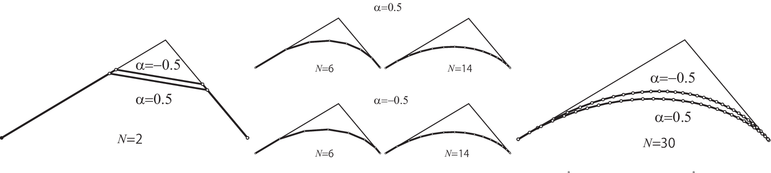
Figure 8 illustrates the examples of dLACs generated by the above method. Despite the different values, the shape of the curves in the top and bottom rows of the middle picture are similar. When (total number of vertices is ), the triangle cut by the vertices polyline of is a little bit larger than that of as shown in the superimposed figure on the left. The right figure illustrates the case of for and the area bounded by the control polyline with the curve for is larger than that with the one for , that is consistent with the left and middle figures. Each curve reasonably approximates its continuous counterpart and the difference of those curves is reasonable when compared with the case of continuous LAC as in [18]. The discrete curvature of the curves (see Remark 5.1) is monotonically increasing from left to right and reproducing continuous LAC’s property very well. The computation time to generate dLAC on a Core i7 6700 3.4GHz is from to msec according to to implemented in Matlab®. The computation time based on numerical discretization of continuous LAC described in [18] takes about msec in Matlab® and the discrete implementation is much faster since fine numerical integration to obtain the shape of the curves is not required and only coarse summation expressed in (73) to keep the boundary conditions is necessary.
The above advantage may be understood to be due to the geometric characterization of dLAC themselves as discrete curves. Namely, in the similarity geometry, the turning angles of the discrete plane curves are constant , so that the shape is controlled by the segment length . Since a discrete analogue of the curvature is given by , which is the reciprocal of the radius of the osculating circle touching the three consecutive edges (see Remark 5.1), if the curvature is large (resp. small) the segment length is small (resp. large). Therefore the distribution of the vertices is dense (resp. coarse) where the curvature is large (resp. small), which implies that the discrete plane curve under the similarity geometry is regarded as a self-adaptive discretization. Even a coarse discrete curve can generate sufficiently good shape. Especially, during the design stage, a designer tries to generate as various as possible curves as to pursue the desired shape. Coarse discrete curves are good enough and desirable because one can generate curves quickly and check their suitability.
7.2 dLAC with an inflection
In this section, we propose a method of generating dLAC with an inflection, i.e. -shaped dLAC based on the similarity geometry.
Unlike the case where there is no inflection as discussed in Section 7.1, here, uniqueness of the solution is not guaranteed. As in the previous section, we assume that the discrete curve has -vertices (). Suppose that for given the turning angles at the vertices are a constant , and those at are . The edge corresponds to the “inflection edge” where the turning angles change the sign at the left and right vertices. We put so that there are vertices to the left of the inflection edge and vertices on the right.

The Euclidean curvature of smooth LAC with an inflection point is given by [11]
| (75) |
where , are parameters. For the similarity curvature of the LAC (10), the unsigned curvature radius is computed by using (8) as
| (76) |
where
| (77) |
and , , are parameters. Moreover, corresponds to the value of the angle function at the inflection point. As mentioned in Remark 5.1, a discrete analogue of the curvature radius for the similarity arc length parametrized discrete plane curve is given by , where is the segment length. In view of this and Definition 5.2 applied to the two parts of the dLAC, we introduce () as
| (78) |
where are parameters to be determined. Then () satisfies the following equations:
| (79) | ||||
| (80) | ||||
| (81) |
From (81) we have
| (82) |
For a given number of vertices , the slope , the endpoints , , the angles at , respectively, and the index of the inflection, one can compute the pair by solving (79) and (80) and the dLAC with an inflection can be generated accordingly. It should be remarked that in the discrete case, must be prescribed and cannot be determined from the equations, so that the dLAC cannot be uniquely determined, while in the smooth case LAC with an inflection point can be uniquely determined under a certain moderate condition [11].
However, if we prescribe the index of the inflection, sometimes there is no solution , or the triplet generates a discrete curve with undesirable shape as illustrated in Figure 10. Therefore, we impose the following assumptions in order to guarantee the existence of the solution and to exclude discrete curves of the type displayed in Figure 10:
| (83) | ||||
| (84) |


Equations (83) and (84) are for excluding the dLACs on the left and on the right of Figure 10, respectively. We remark, however, that it is possible to control the number of loops if desired. Then, we have the following restriction for the index of the inflection, that is, even though is still not unique, it is restricted considerably in the following manner:
Lemma 7.1.
Assume that . Then we have the following estimate:
| (85) |
Proof.
We consider the first case. From the conditions (82), (83) and , we have
Since the assumptions and give , we have
Therefore we conclude
where we used the condition . The remaining part of the estimate can be shown in a similar manner. By the assumption (84), we have
The condition implies that the numerator of the last expression is non-negative, and therefore we have
which proves the first case. The second case is proved in a similar manner noting that . ∎
Note that it is straightfoward to deduce that the indices of inflection satisfying (82) exist if
| (86) |
In summary, one can compute to generate dLAC with an inflection from the given data for each in the relevant range (85) as follows:
This computation generates several dLACs and the choice may be left to the user, but a criteria may be given as follows. Consider the discrete fairing energy
| (87) |
whose Euler-Lagrange equation is given by
| (88) |
Proposition 7.2.
The discrete fairing energy for dLAC with an inflection (78) is given by
| (89) |
Proof.
We first note that we have from (78)
| (90) |
and that satisfies
| (91) |
The constant in (88) for dLAC can be computed by using (90) as
| (92) |
Then we see by using (91) that
| (93) |
where we used . We also have by using (90) and (92)
| (94) |
Then, noticing by (90) that
| (95) |
we obtain from (93), (94) and (95)
| (96) |
which proves the statement. ∎
We may choose the dLAC that attains the minimum of the discrete fairing energy (89). Practically, we may choose the dLAC corresponding to the maximum value of among those generated, since (89) is monotonically decreasing with respect to for each , and the change of the energy with respect to is much smaller than that with respect to .
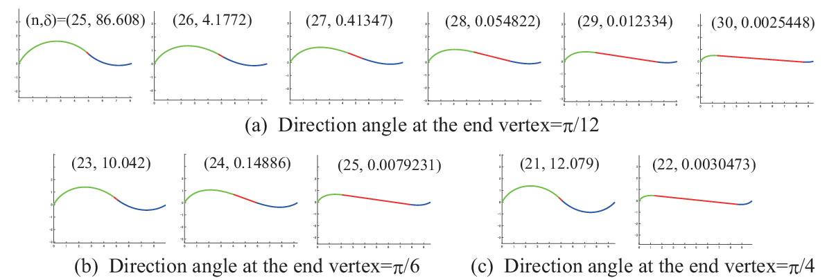
Figure 11 shows various dLAC examples with an inflection edge. We specified , so the total number of the vertices is . and the direction angle at the start (left) vertex is equal to . We changed the direction angle at the end (right) vertex to be , and . The edge in red is an inflection edge in each curve. The sign of the discrete turning angle of the curve segment in green is negative and that in blue is positive. For , there are 6 solutions for , while for and , and solutions exist, respectively. For each curve, we described its corresponding values. As increases, decreases. The discrete fairing energy is the lowest for the left curve in each group, in which its inflection edge is the shortest.
Remark 7.3.
More rigourously, the summation of the fairing energy (87) for the dLAC with an inflection should be taken separately for the left and right sides of the inflection, respectively, and so the variation with the boundary conditions in Theorem 6.1 imposed on both cases. The Euler-Lagrange equation (88) covers the case of in (91), but not the case of . Nervertheless, the computations in the above proof is valid, and the criterion of choosing the largest implies the smallest , which seems natural. This is an intricate problem and more analysis needs to be done to make a rigorous statement. This problem will be dealt with in a future publication.
.
Acknowledgment
This work was supported by JST CREST Grant Number JPMJCR1911. It was also supported by JSPS KAKENHI Grant Numbers JP19K03461, JP19H02048, JP25289021, JP16H03941, JP16K13763, JP15K04834, JP26630038, JST RISTEX Service Science, Solutions and Foundation Integrated Research Program, and ImPACT Program of the Council for Science, Technology and Innovation. The authors acknowledge the support by IMI Joint Use Program Short-Term Joint Research “Differential Geometry and Discrete Differential Geometry for Industrial Design” (September 2016) and “New developments of Discrete Differential Geometry: from industrial design to architecture” (September 2018). The authors would like to express their sincere gratitude to Prof. Miyuki Koiso, Prof. Hiroyuki Ochiai, Prof. Nozomu Matsuura and Prof. Sampei Hirose for invaluable comments and fruitful discussions.
References
- [1] Chou, K.-S., Qu, C.-Z.: Integrable equations arising from motions of plane curves. Phys. D 162, 9–33 (2002). https://doi.org/10.1016/S0167-2789(01)00364-5
- [2] Harada, T., Mori, N. and Sugiyama, K., Curves’ physical characteristics and self-affine properties, Design Study 42(3), 30–40(1995) (in Japanese)
- [3] Harada, T., Study of Quantitative Analysis of the Characteristics of a Curve, Forma 12(1) 55-63(1997).
- [4] Hirota, R.: Nonlinear partial difference equations. V: Nonlinear equations reducible to linear ones, J. Phys. Soc. Japan. 49, 312–319 (1979). https://doi.org/10.1143/JPSJ.46.312
- [5] Hoffmann, T.: Discrete Differential Geometry of Curves and Surfaces, MI Lecture Notes 18, Kyushu University, Fukuoka (2009).
- [6] Inoguchi, J.: Attractive plane curves in differential geometry. In: Dobashi, Y., Ochiai, H. (eds.) Mathematical Progress in Expressive Image Synthesis III. Mathematics for Industry, vol 24, pp. 121–135. Springer, Singapore (2016). https://doi.org/10.1007/978-981-10-1076-7_13
- [7] Inoguchi, J., Kajiwara, K., Miura, K.T., Sato, M., Schief, W.K., Shimizu, Y.: Log-aesthetic curves as similarity geometric analogue of Euler’s elasticae. Comput. Aided Geom. Des. 61, 1–5 (2018). https://doi.org/10.1016/j.cagd.2018.02.002
- [8] Inoguchi, J., Ziatdinov, R., Miura, K.T.: Generalization of log-aesthetic curves via similarity geometry. Japan J. Indust. Appl. Math. 36, 239–259 (2019). https://doi.org/10.1007/s13160-018-0335-7
- [9] Kajiwara, K., Kuroda, T., Matsuura, N.: Isogonal deformation of discrete plane curves and discrete Burgers hierarchy. Pac. J. Math. Ind. 8:3, 14 pages (2016). https://doi.org/10.1186/s40736-016-0022-z
- [10] Miura, K.T.: A general equation of aesthetic curves and its self-affinity. Comput.-Aided Design Appl. 3(1-4) , 457–464 (2006). https://doi.org/10.1080/16864360.2006.10738484
- [11] Miura, K.T., Shibuya, D., Gobithaasan, R.U., Usuki, S.: Designing log-aesthetic splines with G2 Continuity. Comput.-Aided Design Appl. 10(6), 1021–1032 (2013).
- [12] Miura, K.T., Gobithaasan R.U.: Aesthetic curves and surfaces in computer aided geometric design. Int. J. of Automation Technol. 8(3), 304–316 (2014). https://doi.org/10.20965/ijat.2014.p0304
- [13] Miura K.T., Gobithaasan R.U: Aesthetic design with log-aesthetic curves and surfaces. In: Dobashi, Y., Ochiai, H. (eds.) Mathematical Progress in Expressive Image Synthesis III. Mathematics for Industry, vol 24, pp.107–119. Springer, Singapore (2016). https://doi.org/10.1007/978-981-10-1076-7_12
- [14] Nishinari, K., Takahashi, D.: Analytical properties of ultradiscrete Burgers equation and rule-184 cellular automaton. J. Phys. A. Math. Theoret. 31, 5439–5450 (1998). https://doi.org/10.1088/0305-4470/31/24/006
- [15] Sato M., Shimizu, Y.: Log-aesthetic curves and Riccati equations from the viewpoint of similarity geometry. JSIAM Letters 7, 21–24 (2015). https://doi.org/10.14495/jsiaml.7.21
- [16] Sato, M., Shimizu, Y.: Generalization of log-aesthetic curves by Hamiltonian formalism. JSIAM Letters 8, 49–52 (2016). https://doi.org/10.14495/jsiaml.8.49
- [17] Suzuki, T.: Application of log-aesthetic curves to the roof design of a wooden house. Archi-Cultural Interactions through the Silkroad, 4th International Conference, Mukogawa Women’s University, Nishinomiya, Japan, July 16-18, 2016, Selected Papers 121–126 (2017).
- [18] Yoshida, N., Saito, Y.: Interactive aesthetic curve segments. Visual Comput. 22, 896–905 (2006). https://doi.org/10.1007/s00371-006-0076-5