Shape tensor and geometry of embedded manifolds

In this article we are concerned with both intrinsic and extrinsic geometry of manifolds of arbitrary dimension embedded in an arbitrary-dimensional Euclidean space. The central object of this study, the shape tensor, is introduced, and its basic properties are reviewed, in Sec. II. The shape tensor is closely related to the second fundamental form of a surface, and its significance for the study of differentiable manifolds was emphasized by D. Hestenes in his work on geometric algebra and calculus [1, 2].

In Sec. III, the parallel transport is defined as a process when infinitesimal rotations implemented by the shape tensor are used to maintain tangency of vectors transported along the manifold. In this way we reproduce the standard Levi-Civita transport of classical differential geometry. The covariant derivative and curvature are then defined in a standard way in Secs. IV and V. Importantly, the prescription for covariant derivative can be directly applied to both tangent and transverse vectors. As a consequence, the curvature naturally splits into two parts — the intrinsic and the extrinsic one. The shape-tensor-based approach therefore automatically encodes both intrinsic and extrinsic geometry of an embedded manifold.

Frames and coordinates play little role in our discussion, however, we use them in Sec. VI to make contact with the traditional treatment of differential geometry of surfaces, in particular, to recover the connection coefficients.

In Sec. VII the concept of shape-minimizing curves is introduced. They are defined as curves connecting two given points, for which integrated value of the shape tensor magnitude is minimal. (This should be compared to the definition of geodesics as distance-minimizing curves.)

Finally, we provide three examples in Sec. VIII to illustrate the ease and clarity of calculations when employing the shape tensor and geometric algebra techniques. It is advisable to consult the corresponding parts of these examples after each section of the article.

Apart from Sec. VII, this work is largely inspired by (and for the most part summarizes the results of) monographs [1] and [3] about the mathematical language of geometric algebra and calculus, and its use in pure and applied mathematics and in physics. Although we do not attempt to provide a thorough introduction into this formalism, we do recall the basic definitions in Appendix A in the scope necessary for understanding the main text.

Let $\mathcal{M}$ be a smooth $n$-dimensional manifold embedded in the Euclidean space $\mathbb{R}^{N}$. At each point $x\in\mathcal{M}$, we identify the tangent space $T_{x}\mathcal{M}$, including a choice of its orientation, with a simple unit multivector of grade $n$, $I_{\mathcal{M}}(x)$. $I_{\mathcal{M}}$ is referred to as the pseudoscalar of manifold $\mathcal{M}$. It is a smooth function of $x$ provided $\mathcal{M}$ is smooth. ¹¹ 1 Each tangent space possesses two unit pseudoscalars, which differ by a minus sign. Manifolds are orientable if $I_{\mathcal{M}}(x)$ is a single-valued function, and we shall assume this to be the case throughout the text.²² 2 The mapping $x\mapsto I_{\mathcal{M}}(x)$ generalizes the Gauss map that assigns to every point on $\mathcal{M}$ the corresponding normal vector, but which is uniquely defined only if the codimension of $T_{x}\mathcal{M}$ is one.

At each point $x\in\mathcal{M}$, we define the shape tensor ³³ 3 The function defined by Eq. (1) is referred to as the curl of the manifold in Ref. [1], whereas the term ‘shape tensor’ is reserved for a more general object. Our use of the term ‘shape tensor’ is in accordance with Ref. [3, Ch. 6.5.3]. as the directional derivative

where $a$ is a tangent vector at $x$. $S(a;x)$ is therefore a linear function of $a$, and a generic function of $x$. It is illuminating to choose a frame of orthonormal tangent vector fields to express the pseudoscalar as $I_{\mathcal{M}}=e_{1}\ldots e_{n}$, and cast

Here, $\mathsf{P}$ is the operator of projection onto the tangent space, $\mathsf{P}_{\perp}$ is the projection onto the transverse space (the orthogonal complement of the tangent space in the ambient space $\mathbb{R}^{N}$), and we have use the fact that $a\cdot\partial e_{k}$ is perpendicular to $e_{k}$ due to the normalization condition $e_{k}^{2}=1$. In the last expression, the Einstein summation over the repeated index is implied.

The representation (2) makes it obvious that $S(a)$ is a bivector (in general not simple) that consists of terms of the form (tangent vector)$\wedge$(transverse vector) (see Fig. 1). The latter observation implies that $S(a)$ anticommutes ⁴⁴ 4 This can be derived also by differentiating the equation $I_{\mathcal{M}}^{-1}I_{\mathcal{M}}=1$, and taking into account that $I_{\mathcal{M}}^{-1}=(-1)^{n(n-1)/2}I_{\mathcal{M}}$. with $I_{\mathcal{M}}$,

and so we can write

We realize that the shape tensor can be interpreted as the angular velocity of the pseudoscalar $I_{\mathcal{M}}$ as it slides along the manifold, i.e., as the bivector field that implements infinitesimal rotations keeping $I_{\mathcal{M}}$ tangent. ⁵⁵ 5 For hypersurfaces, i.e., submanifolds of dimension $N-1$, dotting Eq. (2) with a tangent vector $b$ and the unit normal $n$ gives $n\cdot\big(b\cdot S(a)\big)=n\cdot(a\cdot\partial b)$ — the second fundamental form of $\mathcal{M}$ [4, Ch. 11.4].

Finally, let us remark that for a pair of tangent vector fields $a$ and $b$, the Lie bracket $[a,b]=a\cdot\partial\,b-b\cdot\partial\,a$ is again tangent, and Eq. (2) thus implies the following symmetry property of the shape tensor:

Parallel transport along the manifold $\mathcal{M}$ can be defined in an intuitive way using the shape tensor. Suppose $A(x)$ is a multivector at some point $x$ (which may contain tangent as well as transverse components), and define the parallel-transported multivector at a close point ${x+\varepsilon a\in\mathcal{M}}$ by composing parallel transport in the ambient Euclidean space, and infinitesimal rotation by the bivector $S(a)$ (see Fig. 2):

According to this definition the pseudoscalar $I_{\mathcal{M}}$ is parallel transported along $\mathcal{M}$ (cf. Eq. (4)). Since rotations commute with the geometric product (and hence with any other product composed from the geometric product, such as $``\cdot"$, $``\wedge"$ or $``\times"$), the parallel transport preserves tangency and transversality, as well as the inner product between vectors. ⁶⁶ 6 For example, if $v(x)$ is tangent at $x$, i.e., $v(x)\wedge I_{\mathcal{M}}(x)=0$, at a nearby point we find $$v(x+\varepsilon a)\wedge I_{\mathcal{M}}(x+\varepsilon a)=e^{-\frac{\varepsilon}{2}S(a)}v(x)\wedge I_{\mathcal{M}}(x)e^{\frac{\varepsilon}{2}S(a)}=0.$$ ⁷⁷ 7 In an alternative definition of the parallel transport, tangent vectors are kept tangent by projection onto the tangent space of the manifold: $$v(x+\varepsilon a)=v(x)\cdot e_{j}(x+\varepsilon a)e_{j}(x+\varepsilon a).$$ Here, $e_{j}$’s form an orthonormal frame, and $v$ is assumed to be tangent at point $x$. Expanding the right-hand side we find $$\frac{1}{\varepsilon}\big(v(x+\varepsilon a)-v(x)\big)\approx v\cdot(a\cdot\partial e_{j})e_{j}+v\cdot e_{j}a\cdot\partial e_{j}=-v\cdot e_{k}\mathsf{P}(a\cdot\partial e_{k})+v\cdot e_{k}a\cdot\partial e_{k}=v\cdot\big(e_{k}\wedge\mathsf{P}_{\perp}(a\cdot\partial e_{k})\big),$$ which agrees with Eq. (6) by virtue of Formula (2).

By Eq. (6), a multivector $A$ is parallel-transported along a curve $\gamma\subset\mathcal{M}$ (whose unit tangent vector we denote by $u$), if

In particular, if $u$ itself is parallel-transported, i.e., $u\cdot\partial u=u\cdot S(u)$, then $\gamma$ is a geodesic.

In order to achieve a finite parallel transport we integrate the infinitesimal rotations of Eq. (6) along $\gamma$ to obtain a finite rotor $R_{\gamma}$, which takes $A(x)$ at some point $x$ into a parallel multivector $A(x^{\prime})=R_{\gamma}(x^{\prime})A(x)\widetilde{R}_{\gamma}(x^{\prime})$. It satisfies $R_{\gamma}(x+\varepsilon u)=e^{-\frac{\varepsilon}{2}S(u;x)}R_{\gamma}(x)$, $\forall x\in\gamma$, or in other words, the differential equation

The solution of this equation can be expressed as a path-ordered exponential

where $d\Gamma=u|d\Gamma|$ is the line element of the curve $\gamma$.

The parallel transport between $x$ and $x^{\prime}$ typically depends upon the choice of path between the two points, since different paths encounter different bivectors $S(u)$ along the way. In explicit terms, $R_{\gamma}(x^{\prime})\neq R_{\gamma^{\prime}}(x^{\prime})$ in general. ⁸⁸ 8 When we consider closed loops $\gamma$, the rotors $R_{\gamma}$ form the holonomy group of the manifold $\mathcal{M}$.

With the notion of parallel transport in hand, one defines the covariant derivative of a multivector field $A(x)$ in a direction $a$ as the difference between the result of the parallel transport of $A$ from a nearby point $x+\varepsilon a$ to $x$, and the value of $A$ at $x$:

Since the parallel transport preserves tangency and transversality of objects it acts on, so does the covariant derivative. Comparison with Eq. (6) shows that $A$ is parallel-transported in direction $a$ if and only if the covariant derivative $a\cdot DA$ vanishes.

Several properties of the covariant derivative follow easily.

If $v$ is a tangent vector field, $v\cdot S(a)$ is transverse, and so the projection of Eq. (10) onto the tangent space yields ⁹⁹ 9 Recall that the commutator product of a vector and a bivector reduces to the inner product: $v\times S(a)=v\cdot S(a)$.

Likewise, for a transverse vector field $w$, the expression $w\cdot S(a)$ is a tangent vector, and we find

The covariant Leibniz rule is a consequence of the Leibniz rule for ordinary derivatives, and identity (60):

Mere rewriting of Eq. (4) demonstrates that the pseudoscalar of manifold $\mathcal{M}$ is covariantly conserved,

Another important result concerns covariant derivative of the shape tensor. From its definition (1), and the anticommutation property (3), we find

where $a$ and $b$ are arbitrary tangent vector fields.

Curvature of a manifold is introduced as a measure of non-commutativity of covariant derivatives in different directions. Therefore, let $A$ be a ‘test’ multivector field, and let us calculate

We have used the definition of covariant derivative, Eq. (10), the covariant Leibniz rule, Eq. (13), the identity (15), and, finally, the Jacobi identity (61). The final result features the quantity

which we call (in agreement with [1, Ch. 5-1]) the (total) curvature. It is an $x$-dependent bivector-valued linear function of a tangent bivector argument. ¹⁰¹⁰ 10 The last claim can be understood with a help of an orthonormal basis of the tangent space, since one can then write explicitly $$S(a)\times S(b)=\frac{1}{2}(a\wedge b)\cdot(e_{j}\wedge e_{k})S(e_{k})\times S(e_{j}).$$ ¹¹¹¹ 11 Eq. (17) defines $\Omega$ only for simple bivectors $a\wedge b$, but we may linearly extend the definition to all tangent bivectors.

The total curvature, being a commutator product of two bivectors of the form (tangent vector)$\wedge$(transverse vector), is a sum of a purely tangent bivector, and purely a transverse bivector. ¹²¹² 12 This becomes clear once we realize that for two bivectors $v_{1}\wedge w_{1}$ and $v_{2}\wedge w_{2}$, where $v_{1}$, $v_{2}$ are tangent and $w_{1}$, $w_{2}$ transverse, $$(v_{1}\wedge w_{1})\times(v_{2}\wedge w_{2})=-v_{1}\cdot v_{2}\,w_{1}\wedge w_{2}-w_{1}\cdot w_{2}\,v_{1}\wedge v_{2}.$$ The tangent, or intrinsic, part is commonly referred to as the Riemann tensor

The transverse, or extrinsic, part of the curvature is denoted by

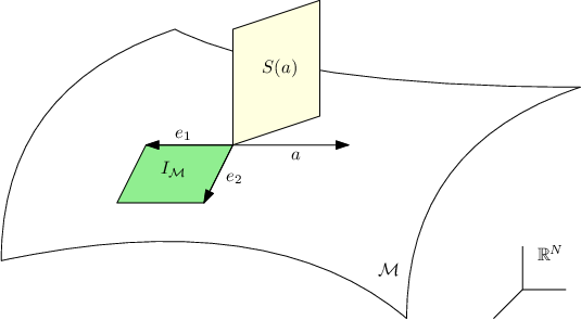
[See the cartoon representation of Fig. 3.]

Note that since the shape tensor lies partly in the tangent and partly in the transverse space, its scalar product with the curvature bivector always vanishes.

In this section we choose, smoothly at each point of the manifold, a basis $\{e_{j}\}_{j=1}^{n}$ of the tangent space, and a basis $\{e_{b}\}_{b=n+1}^{N}$ of the transverse space. The vector fields ${e}_{1},\ldots,{e}_{n}$ form a tangent frame, while the fields $e_{n+1},\ldots,e_{N}$ form a transverse frame. The respective reciprocal frames consist of the unique vector fields $\{e^{j}\}_{j=1}^{n}$ and $\{e^{b}\}_{b=n+1}^{N}$ that satisfy

With the basis decomposition of a generic vector $v=v^{j}e_{j}+v^{b}e_{b}$, where the components $v^{j}=v\cdot e^{j}$ and $v^{b}=v\cdot e^{b}$ are scalar functions, we may cast the covariant derivative as

where

are the connection coefficients in the tangent and transverse space, respectively. [We have used the covariant Leibniz rule, and Eqs. (11) and (12).]

There is a preferred basis of the tangent space when local coordinates on $\mathcal{M}$ are given — the coordinate frame $\{\mathsf{e}_{j}\}_{j=1}^{n}$, with the property $[\mathsf{e}_{j},\mathsf{e}_{k}]=0$. The coefficients $\Gamma(a)_{j}^{k}$ are then the Christoffel symbols, which can be expressed in terms of the metric $g_{ij}=\mathsf{e}_{i}\cdot\mathsf{e}_{j}$, and its inverse $g^{ij}=\mathsf{e}^{i}\cdot\mathsf{e}^{j}$ in a standard way.

Another option to specify frames is to demand that the scalar products $e_{j}\cdot e_{k}$, $e_{b}\cdot e_{c}$ be constant in $x$ for all $j,k,b,c$. We assume this to be the case until the end of this section. The covariant derivative can now be cast in a somewhat more transparent form

where

are tangent- and transverse-space bivectors, respectively (see Fig. 4). They are referred to as the connection bivectors.

Working out now the commutator of covariant derivatives, we obtain an expression for the intrinsic and extrinsic curvatures in terms of $\omega$ and $A$:

Yet another representation is derived by utilizing the bivector bases $e_{J}=e_{j_{1}}\wedge e_{j_{2}}$, $e_{B}=e_{b_{1}}\wedge e_{b_{2}}$, and their reciprocals $e^{J}=e^{j_{2}}\wedge e^{j_{1}}$, $e^{B}=e^{b_{2}}\wedge e^{b_{1}}$ to expand

where $\omega(a)^{J}=\omega(a)\cdot e^{J}$ and $A(a)^{B}=A(a)\cdot e^{B}$. [Summations over repeated multi-indices $J=(j_{1},j_{2})$, $j_{1}<j_{2}$, and $B=(b_{1},b_{2})$, $b_{1}<b_{2}$, are implied.] Note that for $v=e_{j}$ Eq. (23) simplifies to $a\cdot De_{j}=e_{j}\cdot\omega(a)$, and the covariant Leibniz rule then gives $a\cdot De_{J}=e_{J}\times\omega(a)$. Analogously, $a\cdot De_{B}=e_{B}\times A(a)$. We thus find

and finally arrive at

In analogy with geodesics, i.e., curves that minimize distance between two given points $x_{1}$ and $x_{2}$, let us study curves that minimize the functional

where $d\Gamma$ is the oriented line element of a curve $\gamma$, which can be written as a product $d\Gamma=u|d\Gamma|$ of the unoriented line element $|d\Gamma|$, and the unit tangent vector $u$. We refer to curves that minimize the functional $\Sigma[\gamma]$ as shape-minimizing curves.

Let $\gamma^{\prime}=\{x+\varepsilon a(x)\,|\,x\in\gamma\}$ be a variation of $\gamma$, governed by a vector field $a$, that fixes the endpoints: $a(x_{1})=a(x_{2})=0$. The line element and the shape tensor are varied as follows:

and

Taking into account Eq. (15), we can further rearrange

Variation of the functional $\Sigma[\gamma]$ is carried out conveniently with a help of Formula (70),

where we have made integration by parts, and noticed that $\widetilde{S}(d\Gamma)\cdot(S(d\Gamma)\times S(a))=0$ since the scalar product between the curvature and the shape bivectors always vanishes. (They belong to different bivector subspaces.) Extremal curves satisfy the differential equation

for all tangent vectors $a$.

The derivation, and the final equation (34), only make sense under the assumption $|S(u)|>0$. The expression $\widetilde{S}(a)\cdot S(b)$ can be understood as an alternative metric on the manifold $\mathcal{M}$, which, however, may well be degenerate. ¹³¹³ 13 Note that for a plane (for example), the shape tensor identically vanishes, and so all curves have the same value of $\Sigma[\gamma]$, which is equal to 0.

The partial derivative $u\cdot\partial$ in Eq. (34) can be replaced by a covariant derivative $u\cdot D$, as these two only differ by a term proportional to $S(u)\times S(u)=0$. Then, it is clear that the bivector in the square bracket is composed of terms of the form (tangent vector)$\wedge$(transverse vector). Therefore, if the space of such bivectors is spanned by the shape bivectors $S(a)$, which will be the case in Example VIII.3, Eq. (34) is equivalent to

In this article we reintroduced some basic concepts of differential geometry (parallel transport, covariant derivative, curvature) in the case of embedded manifolds. We did so with a help of the shape tensor — an object, which encodes intrinsic as well as extrinsic geometry of the manifold.

In analogy with geodesics, we introduced shape-minimizing curves as extremals of the functional that measures the ‘shape’-distance, i.e., the integrated value of the shape tensor magnitude accumulated along the path. They have been found explicitly on a generic ellipsoid.

To phrase the presented ideas in a more abstract setting, one may consider an $N$-dimensional vector bundle over an $n$-dimensional base manifold $\mathcal{M}$, together with a map relating the tangent spaces $T_{x}\mathcal{M}$ with certain $n$-dimensional subspaces of the fibres. The complements of these subspaces are then the transverse spaces. Over each fibre we can introduce a geometric algebra, and the shape tensor can be regraded as a one-form with values in its bivector part. Further details shall be discussed in a separate article.

References

- [1] D. Hestenes and G. Sobczyk, Clifford Algebra to Geometric Calculus, Springer (1987).
- [2] D. Hestenes, The Shape of Differential Geometry in Geometric Calculus, In: L. Dorst and J. Lasenby (eds.), Guide to Geometric Algebra in Practice, Springer, London (2011).
- [3] C. Doran and A. Lasenby, Geometric Algebra for Physicists, Cambridge Univ. Press (2007).
- [4] T. Frankel, The Geometry of Physics: An Introduction, 2nd. Ed., Cambridge Univ. Press (2004).
- [5] W. Klingenberg, Riemannian Geometry, W. de Gruyter (1982).