Advances in Distributed Graph FilteringThanks: The authors are with the faculty of Electrical Engineering, Mathematics and Computer Science, Delft University of Technology, 2826 CD Delft, The Netherlands. E-mails: $\{$m.a.coutinominguez, e.isufi-1, g.j.t.leus$\}$@tudelft.nl. This research is supported in part by the ASPIRE project (project 14926 within the STW OTP programme), financed by the Netherlands Organization for Scientific Research (NWO). Mario Coutino is partially supported by CONACYT. A conference version of this work was presented in [1].

Driven by the practical need to implement a linear function with few local operations, the works in [9, 27] have put efforts to ease the communication and computational costs of graph filters (GF).

In [9], the authors modified the polynomial graph filters (i.e., the FIR structure) to graph filters with node-dependent weights. This architecture, referred to as a node-variant (NV) FIR graph filter, assigns different weights to different nodes and yields the same distributable implementation as the classical FIR graph filter [6, 4]. The NV FIR filter addresses a broader family of linear operators (e.g., analog network coding) that goes beyond the class of shift-invariant graph filters. However, the NV FIR filter uses the same weight for all signals arriving at a particular node, ignoring the affinity between neighbors. As we show next, this limits the ability of the NV FIR filter in approximating the desired linear operator with very low orders.

The work in [27] introduced stochastic sparsification to reduce the cost of a distributable implementation. Here, the authors considered random edge sampling in each aggregation step to implement the filter output with a lower complexity. Although conceptually similar to this work, the filter following [27] is stochastic and, therefore, the results hold only in expectation. Moreover, since this approach applies only to shift invariant filters, such as the FIR filter [6, 4] and the IIR [10] implementations, it cannot address linear operators that are not shift invariant.

Another related problem, which can be interpreted like graph filtering, is the multilayer sparse approximation of matrices [28]. Different from the previous two approaches, here a dense linear transform (matrix) is approximated through a sequence of sparse matrix multiplications to obtain a computational speedup. While this framework can be considered as sequential diffusions over a network, the support of such sparse matrices differs in each iteration. This in practice can be a limitation since it often requires information from non-adjacent nodes within an iteration. Finally, in [29] the problem of optimal subspace projection by local interactions was studied. This paper proposed an algorithm to design the weights of a network to achieve the fastest convergence rate for this kind of linear operators. Although their method provides optimal weights for projecting the data to a particular subspace, it does not address the GSP setup of interest: implementation of graph filters or general linear operators.

The main contribution of this work is the extension of the state-of-the-art graph filters to edge-variant (EV) graph filters. Due to the increased degrees of freedom (DoF), these filters allow for a complexity reduction of the distributed implementation while maintaining the approximation accuracy of current approaches. The salient points that broaden the existing literature are listed below.

• –

  We present edge-variant architectures to implement FIR and IIR graph filtering. This framework extends the state-of-the-art graph filters by allowing nodes to weigh differently the information coming from different neighbors. In this way, only local exchanges are needed for each shift, thus yielding an efficient distributable implementation. Three forms are analyzed: First, the general class of linear edge-variant FIR filters is presented and its distributable implementation is discussed. Then, following the per-tone equalization idea [30], the constrained edge-variant FIR graph filter is introduced. This filter maintains a similar distributable implementation as the general form, yet allowing a simple least-squares design. Finally, the family of edge-variant autoregressive moving average graph filters of order one (ARMA₁) is treated. This new IIR distributable architecture allows a better trade-off between approximation accuracy and convergence rate than current approaches.

• –

  Through the definition of the filter modal response, we give a Fourier interpretation to a particular family of edge-variant graph filters. This subfamily shows a shift-invariant nature and links the filtering operation with the scaling applied on the graph modes (e.g., the graph shift eigenvectors).

• –

  Besides outperforming state-of-the-art graph filters in GSP tasks such as approximating a user-provided frequency response, distributed consensus, and Tikhonov denoising, we present two new applications that could be addressed distributively with the proposed edge-variant graph filter. The latter includes a distributed solution of an inverse problem and distributed beamforming.

This paper is organized as follows: Section II reviews the preliminaries of GSP, distributed graph filtering, and further defines the modal response of a graph filter. Section III generalizes the FIR graph filters to the edge-variant version. Here, we introduce the shift-invariant edge-variant graph filter and characterize its graph modal response. Section IV analyzes a particular subfamily of edge-variant FIR graph filters, which enjoys a similar distributed implementation and a least-squares design strategy. In Section V, we generalize the idea of edge-variant filtering to the class of IIR graph filters. Section VI corroborates our findings with numerical results and Section VII concludes this paper.

In this paper, we adopt the following notation. Scalars, vectors, matrices, and sets are denoted by lowercase letters $(x)$, lowercase boldface letters $(\bm{x})$, uppercase boldface letters $(\bm{X})$, and calligraphic letters $(\mathcal{X})$, respectively. $[\bm{X}]_{ij}$ denotes the $(i,j)$th entry of the matrix $\bm{X}$ whereas $[\bm{x}]_{i}$ represents the $i$th entry of the vector $\bm{x}$. $\bm{X}^{\mathsf{T}}$, $\bm{X}^{\mathsf{H}}$, and $\bm{X}^{-1}$ are respectively the transpose, the Hermitian, and inverse of $\bm{X}$. The Moore-Penrose pseudoinverse of $\bm{X}$ is $\bm{X}^{\dagger}$. The Khatri-Rao product between $\bm{X}$ and $\bm{Y}$ is written as $\bm{X}\ast\bm{Y}$, while their Hadamard product as $\bm{X}\odot\bm{Y}$. $\bm{1}$ and $\bm{I}$ are the all-one vector and identity matrix of appropriate size, respectively. ${\rm vec}(\cdot)$ is the vectorization operation. ${\rm diag}(\cdot)$ refers to a diagoal matrix with its argument on the main diagonal. ${\rm null}\{\cdot\}$ and ${\rm span}\{\cdot\}$ denote the nullspace and span of their argument. ${\rm nnz}(\bm{X})$ and ${\rm supp}\{\bm{X}\}$ are the number of nonzero entries and the support of $\bm{X}$. Finally, we define the set $[K]=\{1,2,\ldots,K\}$.

Consider an extension of the above edge-dependent fusion to several diffusion steps (signal shifts) where in each shift a different set of weights is used. At the $k$th diffusion, node $v_{i}$ weighs its neighbouring node $v_{l}$ with the weight $\phi_{i,l}^{(k)}$. Hence, in each shift $k\in[K]$, and for each node $v_{i}$, there is a set of coefficients $\{\phi_{i,l}^{(k)}\}$ for $l\in\mathcal{N}_{v_{i}}$. Here, $\mathcal{N}_{v_{i}}$ denotes the set of nodes adjacent to $v_{i}$, and $K$ is the number of shifts. Mathematically, the above behavior can be written through an order-$K$ general EV FIR graph filter defined as

where $\bm{\Phi}_{k:1}=\bm{\Phi}_{k}\bm{\Phi}_{k-1}\cdots\bm{\Phi}_{1}$ and $\bm{\Phi}_{j}\in\mathbb{C}^{N\times N}$ is an edge-weighting matrix constructed from the coefficient set $\{\{\phi_{1,l}^{(j)}\},\cdots,\{\phi_{N,l}^{(j)}\}\}$, more specifically $[\bm{\Phi}_{j}]_{il}=\phi_{i,l}^{(j)}$. By construction, the support of $\bm{\Phi}_{j}$ and $\bm{S}+\bm{I}$ is the same $\forall\;j\in[K]$. Since $\bm{S}$ might have zero entries on its diagonal, i.e., $\bm{S}=\bm{W}$, here we extend the support of $\{\bm{\Phi}_{j}\}_{j\in[K]}$ to allow each node to use also its own information. Note that definition (9) does not impose any symmetry on the coefficient matrices $\bm{\Phi}_{j}$. Depending on how adjacent nodes trust each other, the applied weights can be different.

The filter can differently be interpreted through time-varying shift operators [32, 33], where $\bm{\Phi}_{j}$ is the weighted, possibly directed shift operator for the $j$th diffusion step with the support of $\bm{S}+\bm{I}$. Therefore, the general EV FIR filter accounts for signals that are generated through time-varying systems in directed subgraphs of the original graph. Here, the filter coefficient matrix only allows for edge deletion or a re-weighting of graph flows.

Note that recursion (9) is a distributed graph filter. To compute the output $\bm{y}=\bm{H}_{\rm ev}\bm{x}$, each node is only required to track the following quantities:

• •

  the shifted signal output $\bm{x}^{(k)}=\bm{\Phi}_{k}\bm{x}^{(k-1)},\bm{x}^{(0)}=\bm{x}$,

• •

  the accumulator output $\bm{y}^{(k)}=\bm{y}^{(k-1)}+\bm{x}^{(k)},\bm{y}^{(0)}=\bm{0}$.

Both these operations can be computed locally in each node by combining only neighboring data. Hence, (9) preserves the efficient distributed implementation of the classical FIR graph filter (4) with a complexity of $\mathcal{O}(MK)$.

Before addressing the design strategy of the filter (9), in the sequel, we introduce a particular structure of EV FIR graph filters that enjoy a graph Fourier domain interpretation.

An important family of graph filters is that of shift-invariant graph filters, i.e., filters that commute with the graph shift operator $\bm{S}$. That is, given the shift $\bm{S}$ and the filter matrix $\bm{H}$, the following holds

For a non-defective shift operator $\bm{S}$ and filter $\bm{H}$, i.e., the matrices accept an eigenvalue decomposition, condition (10) is equivalent to saying that the matrices $\bm{S}$ and $\bm{H}$ are jointly diagonalizable, or that their eigenbases coincide.

There is no reason to believe that the graph filters of form (9) are shift invariant. However, it is possible to characterize a subset of edge-variant graph filters that satisfy this property. To do that, we rely on the following assumptions:

• $(A.0)$ $\bm{S}$ is diagonalizable;

• $(A.1)$ Each $\bm{\Phi}_{j},\,j\in[K]$ is diagonalizable with the eigenbasis of $\bm{S}$;

• $(A.2)$ Each $\bm{\Phi}_{j},\,j\in[K]$ shares the support with $\bm{S}+\bm{I}$.

Given the above assumptions hold, we can rewrite (9) as

where we substituted $\bm{\Phi}_{j}=\bm{U}\bm{\Lambda}_{j}\bm{U}^{-1}$. To provide a closed-form expression for the effect of such graph filters on the graph modes, let us first describe the set of fixed-support matrices that are diagonalizable with a particular eigenbasis (i.e., matrices that meet $(A.1)$ and $(A.2)$). Mathematically, this set is defined as

where $\mathcal{A}$ is the index set defining the zero entries of $\bm{S}+\bm{I}$ and $\bm{\Omega}$ is diagonal. The fixed-support condition in $\mathcal{J}_{\bm{U}}^{\mathcal{A}}$ can be expressed in the linear system form

with $\bm{\Phi}_{\mathcal{A}}\in\{0,1\}^{|\mathcal{A}|\times N^{2}}$ denoting the selection matrix whose rows are the rows of an $N^{2}\times N^{2}$ identity matrix indexed by the set $\mathcal{A}$. By leveraging the vectorization operation properties and the knowledge of the eigenbasis of $\bm{A}$, we can rewrite (13) as

where “$\ast$” represents the Kathri-Rao product and $\bm{\omega}=[[\bm{\Omega}]_{11},[\bm{\Omega}]_{22},\ldots,[\bm{\Omega}]_{NN}]^{\mathsf{T}}$ is the vector containing the eigenvalues of $\bm{A}$. From (14), we see that $\bm{\omega}$ characterizes the intersection of the nullspace of $\bm{\Phi}_{\mathcal{A}}$ and the range of $\bm{U}^{-\mathsf{T}}\ast\bm{U}$. More formally, we write

with $\bm{T}_{\bm{U}}^{\mathcal{A}}=\bm{\Phi}_{\mathcal{A}}(\bm{U}^{-\mathsf{T}}\ast\bm{U})$.

With this in place, the following proposition characterizes the matrices that belong to the set $\mathcal{J}_{\bm{U}}^{\mathcal{A}}$.

The above result is not entirely surprising and has been used for assessing the uniqueness of the graph shift operator in topology identification [34]. Here, we leverage Proposition 1 for interpreting the response of the SIEV graph filters. More specifically, under $(A.1)$ and $(A.2)$ we can express each matrix $\bm{\Phi}_{j}$ of (9) as

and write any SIEV FIR filter as

The following proposition formally characterizes the frequency interpretation of such filters in terms of the modal response.

An interesting outcome from Proposition 2 is that the filter response is independent of the graph frequencies. This is clear from (19), where we see that the eigenvalue $\lambda_{i}$ does not appear in the expression of $h_{i}$. Therefore, we can interpret the SIEV FIR graph filters as eigenvector filters, since they act on the eigenmodes of the graph. That is, for each graph eigenmode (eigenvector) $\bm{u}_{i}$, $\bm{H}_{\rm siev}$ might apply a different gain given by (19) (independent of $\lambda_{i}$) to the component of the input signal $\bm{x}$ in the direction of $\bm{u}_{i}$. This is in contrast to classical FIR graph filters which apply the same polynomial expression to all modes $\{\bm{u}_{i}\}_{i\in[N]}$.

The following section introduces methods for designing EV FIR graph filters in the node domain and SIEV FIR graph filters using the parametrization in (19).

General form. Given a desired operator $\tilde{\bm{H}}$, we design an EV FIR filter $\bm{H}_{\rm{ev}}$ [cf. (9)] that approximates $\tilde{\bm{H}}$ as the solution of the optimization problem

where $\|\cdot\|$ is an appropriate distance measure, e.g., the Frobenius norm ($\|\cdot\|_{F}$), or the spectral norm ($\|\cdot\|_{2}$).

Unfortunately, (20) is a high-dimensional nonconvex problem and hard to optimize. An approach to finding a local solution for it is through block coordinate methods, which provide local convergence guarantees when applied to such problems [35]. In fact, the cost in (20) is a block multi-convex function, i.e., the cost function is a convex function of $\bm{\Phi}_{i}$ with all the other variables fixed.

Starting then with an initial set of matrices $\{\bm{\Phi}_{j}^{(0)}\}_{j\in[K]}$ (potentially initialized with an order-$K$ classical FIR filter), we solve a sequence of optimization problems where at the $i$th step, the matrix $\bm{\Phi}_{i}$ is found. That is, at the $i$th iteration, we fix the matrices $\{\bm{\Phi}_{j}^{(0)}\}_{j\in[K]\backslash\{i\}}$ and solve the convex problem

where $\bm{\Phi}_{a:b}^{(0)}=\bm{\Phi}_{a}^{(0)}\bm{\Phi}_{a-1}^{(0)}\ldots\bm{\Phi}_{b+1}^{(0)}\bm{\Phi}_{b}^{(0)}$ for $a\geq b$ and $\bm{\Phi}_{a:b}^{(0)}=\bm{I}$, otherwise. Then, the matrix $\bm{\Phi}_{i}^{(0)}$ is updated with its solution and the procedure is repeated for all $\{\bm{\Phi}_{j}\}_{j\in[K]}$. If the final fitting error is large, the whole process can be repeated until the desired performance is reached, or until a local minimum is found.

Although filter (9) is the most general EV FIR filter form, the non-convexity encountered in the above design strategy may often lead to a local solution with an unacceptable performance. To tackle such issue, in Section IV, we introduce a constrained EV FIR filter which provides a higher flexibility than the state-of-the-art graph filters while accepting a simple least squares design.

SIEV form. Besides enjoying the modal response interpretation, the SIEV FIR filter also has a simpler design than the general form (9). For $\{\tilde{h}_{i}\}_{i=1}^{N}$ being the desired graph modal response¹¹ 1 This can be for instance a low-pass form if we want to keep only the eigenvector contribution associated with the low graph frequencies., the SIEV FIR filter design consists of solving the optimization problem

Similarly to (20), problem (22) is nonconvex and cannot in general be solved up to global optimality with standard convex optimization methods. However, (22) is also a block multi-convex function in each $\bm{\alpha}_{i}$, $i\in[K]$ individually and, therefore, the block coordinate descent methods [35] can be employed to find a local minimum. Alternatively, the straightforward analytical expression of the gradient of the cost function allows the use of off-the-shelf solvers for global optimization, such as the MATLAB’s built-in fmincon function [36].

The constrained EV (CEV) FIR graph filter is defined as

where the edge-weighting matrices $\{\bm{\Phi}_{k}\}_{k\in[K]}$ again share the support with $\bm{S}+\bm{I}$. These filters enjoy the same distributed implementation of the general form (9). In fact, each node can compute locally the filter output by tracking the following quantities:

• •

  the regular shift output $\bm{x}^{(k)}=\bm{S}\bm{x}^{(k-1)},~\bm{x}^{(0)}=\bm{x}$,

• •

  the weighted shift output $\bm{z}^{(k)}=\bm{\Phi}_{k}\bm{x}^{(k-1)}$,

• •

  the accumulator output $\bm{y}^{(k)}=\bm{y}^{(k-1)}+\bm{z}^{(k)},~\bm{y}^{(0)}=\bm{0}$.

From the locality of $\bm{S}$ and $\bm{\Phi}_{k}$, both $\bm{x}^{(k)}$ and $\bm{z}^{(k)}$ require only neighboring information. The final filter output is $\bm{y}=\bm{y}^{(K)}$ which yields the same computational complexity of $\mathcal{O}(MK)$.

Note that construction (23) still applies different weights to the signal coming from different edges. However, instead of adopting a different diffusion matrix at every step, the signal diffusion occurs through the graph shift $\bm{S}$. The additional extra step mixes locally $\bm{x}^{(k-1)}$ using edge-dependent weights, which are allowed to vary for each $k$. We here adopt the term constrained for this implementation from the observation that the diffusion is performed using only a single shift operator matrix. Fig. 1(a) visually illustrates the differences between the different graph filters analyzed so far.

Following the same lines of Section III-B, we can use the set $\mathcal{J}_{\bm{U}}^{\mathcal{A}}$ (12) to characterize the graph modal response of the CEV FIR graph filter when the matrices $\{\bm{\Phi}_{k}\}_{k=1}^{K}$ satisfy $(A.1)$ and $(A.2)$. This subset of CEV FIR graph filters, which we refer to as shift-invariant CEV (SICEV) FIR graph filters, can again be expressed in terms of $\bm{B}_{\bm{U}}^{\mathcal{A}}$ and $\{\bm{\alpha}_{k}\}_{k=0}^{K}$ as

where $\bm{\lambda}^{\odot k}$ denotes the $k$th element-wise power of the eigenvalue vector of the shift operator $\bm{S}$. The subsequent proposition formalizes the modal response of these filters.

From (25), we see that there is a substantial difference between the SICEV FIR filter and the more general SIEV FIR graph filters. Here, the modal response is a polynomial in the graph frequencies. This is similar as for the classical FIR filter (4), but now each frequency has a different set of coefficients. In other words, the modal response of the SICEV FIR filter is a mode-dependent polynomial. For readers more familiar with traditional discrete-time processing, this behavior can be interpreted as applying different polynomial filters to each frequency bin (see e.g., [30]).

General form. Following a similar approach as in Section III-C, we can approximate a desired operator $\tilde{\bm{H}}$ with a CEV FIR filter by solving the problem

Exploiting then the properties of the vectorization operator and the Frobenius norm, we can transform (26) into

Since the support of the weighting matrices is known, problem (27) can be written in the reduced-size form

where, $\check{\bm{\phi}}_{k}$ is the vector $\bm{\phi}_{k}$ with the zero entries removed, $\check{\bm{S}}_{k}$ is the matrix $(\bm{S}^{k}\otimes\bm{I})$ with the appropriate columns removed. In addition, if a regularized solution is desired, a natural penalization term might be the convex $\ell_{1}$-norm which induces sparsity in the solution yielding only few active coefficients.

Problem (27) has a unique solution as long as $\bm{\Psi}$ is full column rank, i.e., ${\rm rank}(\bm{\Psi})={\rm nnz}(\bm{S})\cdot K+N$. Otherwise, regularization must be used to obtain a unique solution.

SICEV form. Similar to the more general CEV FIR filter, the design of $\{\bm{\alpha}_{k}\}_{k=1}^{K}$ for the SICEV form can be performed in a least squares fashion.

First, for a set of vectors $\{\bm{\alpha}_{k}\}_{k=1}^{K}$ the modal response for the SICEV FIR filter reads as

where $\bm{h}_{\lambda}$ is obtained by stacking the modal responses, i.e., $\{h_{i}\}_{i=1}^{N}$, in a column vector. By using the properties of the Hadamard product, we can rewrite (29) as

with $\bm{M}_{k}={\rm diag}(\bm{\lambda}^{\odot(k-1)})\bm{B}_{\bm{U}}^{\mathcal{A}}$. Defining then $\bm{M}=[\bm{M}_{1},\ldots,\bm{M}_{K}]$, and $\bm{\alpha}=[\bm{\alpha}_{1}^{\mathsf{T}},\ldots,\bm{\alpha}_{K}^{\mathsf{T}}]^{\mathsf{T}}$, we obtain the linear relation

Therefore, the approximation of a desired response $\tilde{\bm{h}}_{\bm{\lambda}}=~[\tilde{h}_{1},\ldots,\tilde{h}_{N}]^{\mathsf{T}}$ consists of solving the least squares problem

which has a unique solution when $\bm{M}$ is full column rank, i.e., ${\rm rank}(\bm{M})=d(K+1)\leq N$.

We build an edge-variant ARMA₁ recursion on graphs by modifying (6) as

where $\bm{\Phi}_{0}$ and $\bm{\Phi}_{1}$ are the edge-weighting matrices having the support of $\bm{S}+\bm{I}$ that respectively weight locally the entries of $\bm{y}_{t-1}$ and $\bm{x}$. Proceeding similarly as in [10], for $\|\bm{\Phi}_{1}\|_{2}<1$, the steady-state output of (33) is

where now we notice the inverse relation w.r.t. the edge-weighting matrix $\bm{\Phi}_{1}$. Recursion (33) converges to (34) linearly with a rate governed by $\|\bm{\Phi}_{1}\|_{2}$. The classical form (6) can be obtained by substituting $\bm{\Phi}_{1}=\psi\bm{S}$ and $\bm{\Phi}_{0}=\varphi\bm{I}$.

The edge-variant ARMA₁ filter presents the same frequency interpretation challenges as the FIR filter counterpart. Therefore, we next analyze the shift-invariant version of it and we will see a rational modal response.

By limiting the choices of $\{\bm{\Phi}_{0},\bm{\Phi}_{1}\}$ to the one that satisfy $(A.1)$ and $(A.2)$, we obtain the shift-invariant edge-variant ARMA₁ (SIEVA₁) graph filter

where $\bm{\alpha}_{0}$ and $\bm{\alpha}_{1}$ are the respective basis expansion vectors of $\bm{\Phi}_{0}$ and $\bm{\Phi}_{1}$ onto the nullspace of $\bm{T}_{\bm{U}}^{\mathcal{A}}$ (see Proposition 1). From (35), we see that the inverse relation that appears in (34) indeed appears as a function affecting the graph eigenmodes. The following proposition concludes this section by stating this finding in a formal way.

Edge-Variant ARMA₁ form. Here, we extend the design approach of [38] and design $\{\bm{\Phi}_{0},\bm{\Phi}_{1}\}$ by using the Prony’s method. For $\tilde{\bm{H}}$ being the desired operator, we can define the fitting error matrix

which similar to the classical Prony design presents nonlinearities in the denominator coefficients, i.e., in $\bm{\Phi}_{1}$. To tackle these issues, we consider the modified fitting error matrix

which is obtained by multiplying both sides of (37) by $\bm{I}-\bm{\Phi}_{1}$.

This way, the filter design is transformed in solving the convex optimization problem

The objective function in (39) aims at reducing the modified error $\bm{E}^{\prime}$, while the first constraint trades the convergence rate of (33) with approximation accuracy.

SIEVA₁ form. Following the same idea as in (37)-(39), the modified fitting error of a SIEVA₁ graph filter is

with $\tilde{h}_{i}$, $(\bm{b}_{\bm{U},i}^{\mathcal{A}})^{\mathsf{T}}\bm{\alpha}_{0}$, and $(\bm{b}_{\bm{U},i}^{\mathcal{A}})^{\mathsf{T}}\bm{\alpha}_{1}$ denoting respectively the desired modal response and the eigenvalues of $\bm{\Phi}_{0}$ and $\bm{\Phi}_{1}$ w.r.t. the $i$th mode. In vector form, (40) is be written as

with ${\bm{e}^{\prime}}=[e_{1}^{\prime},\ldots,e_{N}^{\prime}]^{\mathsf{T}}$, $\tilde{\bm{h}}_{\lambda}=[\tilde{h}_{1},\ldots,\tilde{h}_{N}]^{\mathsf{T}}$, $\bm{\Psi}_{\lambda}=[\bm{B}_{\bm{U}}^{\mathcal{A}},\;{\rm diag}(\tilde{\bm{h}}_{\lambda})\bm{B}_{\bm{U}}^{\mathcal{A}}]$, and $\bar{\bm{\alpha}}=[\bm{\alpha}_{0}^{\mathsf{T}}\;\bm{\alpha}_{1}^{\mathsf{T}}]^{\mathsf{T}}$. Then, $\{\bm{\alpha}_{0},\bm{\alpha}_{1}\}$ can be estimated as the solution of the constrained least squares problem

Problem (42) again aims at minimizing the modified fitting error, while tuning the convergence rate through $\delta$.

Differently from the general EV-ARMA₁, here the number of unknowns is reduced to $2d$, as now only the vectors $\bm{\alpha}_{0}$ and $\bm{\alpha}_{1}$ need to be designed. Therefore, due to this low dimensionality, one can also opt for global optimization solvers to find an acceptable local minimum of the true error (i.e., the equivalent of (37)).

We here test the proposed FIR graph filters in approximating a user-provided frequency response. We consider a random community graph of $N=256$ nodes and shift operator $\bm{S}=\bm{L}$. The frequency responses of interest are two commonly used responses in the GSP community, i.e.,

• $(i)$

  the exponential kernel

  $$\tilde{h}(\lambda)\coloneqq e^{-\gamma(\lambda-\mu)^{2}},$$

  with $\gamma$ and $\mu$ being the spectrum decaying factor and the central parameter respectively;

• $(ii)$

  the ideal low-pass filter

  $$\tilde{h}(\lambda)=\begin{cases}1&0\leq\lambda\leq\lambda_{\text{c}}\\ 0&\text{otherwise},\end{cases}$$

  with $\lambda_{\text{c}}$ being the cut-off frequency.

The approximation accuracy of the different filters is evaluated in terms of the normalized squared error $\text{NSE}=\|\tilde{\bm{H}}-\bm{H}_{\rm{fit}}\|_{F}^{2}/\|\tilde{\bm{H}}\|_{F}^{2}$. $\bm{H}_{\rm{fit}}$ stands for the filter matrix of the fitted filters.

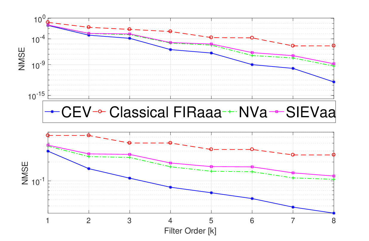
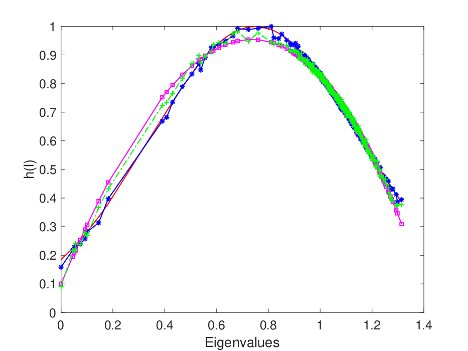
Fig. 2 illustrates the performances of the different filters. In the exponential kernel scenario, we observe that the CEV FIR filter outperforms the other alternatives by showing a performance improvement of up to two orders of magnitude. A similar result is also seen in the low-pass example, where the CEV FIR filter achieves the error floor for $K=8$, while the NV graph filter for $K=13$ and the classical FIR filter for $K=17$. Additionally, we observe that the SIEV FIR filter achieves the same performance as the NV FIR filter. This result suggests that despite the additional DoF of the SIEV FIR filter, the nonconvex design strategy (22) yields in a local minimum that does not exploit the filter full capabilities.

The above observations further motivate the use of the CEV FIR filter, which trades off better the simplicity of the design and the available DoF. In fact, even though the CEV FIR filter has less DoF than the SIEV graph filter, it performs better than the latter. Similarly, the larger DoF of the CEV FIR filter compared to the NV FIR filter (i.e., $\rm{nnz}(\textbf{S})\cdot K+N$ vs $N\cdot(K+1)$) allow the CEV FIR filter to better approximate the desired response. In a distributed setting, these benefits translate into communication and computational savings.

Several distributed tasks of interest consist of performing a linear operation $\bm{A}\in\mathbb{R}^{N\times N}$ over a network. This can be for instance a beamforming matrix over a distributed array or consensus matrix. In most of these cases, such linear operators cannot be straightforwardly distributed. In this section, we illustrate the capabilities of the developed graph filters in addressing this task.

Given a desired linear operator $\bm{A}$, we aim at implementing this linear operator distributively through the solution of the optimization problem

where $\bm{H}(\bm{S},\bm{\theta})$ stands for the used graph filter parametrized by the shift $\bm{S}$ and a set of parameters $\bm{\theta}$ living in the domain $\Theta$.

Distributed Consensus. For distributed consensus, the operator ${\bm{A}}$ has the form ${\bm{A}}=\frac{1}{N}\bm{1}\bm{1}^{T}$, which for $\bm{S}=\bm{L}$ translates into a low-pass graph filter passing only the DC signal component.

Fig. 3 compares the fitting $\text{NSE}=\|\bm{A}-\bm{H}_{\rm{fit}}\|_{F}^{2}/\|\tilde{\bm{H}}\|_{F}^{2}$ for the different FIR graph filters. We note once again that the CEV implementation offers the best approximation accuracy among the contenders achieving an NSE of order $10^{-4}$ in only $10$ exchanges. These results yield also different insights about the SIEV and SICEV graph filters.

First, both the SIEV and the SICEV implementations fail to compare well with the CEV, though the linear operator $\bm{A}$ is shift invariant. We attribute this degradation in performance to assumption (A.1) necessary for these filters to have a modal response interpretation. In fact, forcing each filter coefficient matrix to be shift invariant seems limiting the filter ability to match well the consensus operator.

Second, the different design strategies used in SIEV and SICEV further discriminate the two filters. We can see that the least squares design of the SICEV implementation is more beneficial, though the SIEV filter has more DoF. Unfortunately, this is the main drawback of the latter graph filter, which due to the nonconvexity of the design problem leads to suboptimal solutions. However, we remark that both these filters outperform (or compare equally with) the classical FIR filter. Further investigation in this direction is needed to understand if the SIEV, or SICEV structures can be used to achieve finite-time consensus as carried out in [42, 43].

Wiener-based denoising. For instances when the statistics of the graph signal and noise signal are available, a typical approach for performing denoising is the Wiener filter. This filter is obtained by minimizing the mean-squared error, i.e.,

where $\bm{z}=\bm{x}+\bm{n}$ is the graph signal corrupted with additive noise. For the case of zero-mean signals $\bm{x}$ and $\bm{n}$ with covariance matrices $\bm{\Sigma}_{\bm{x}}$ and $\bm{\Sigma}_{\bm{n}}$, respectively, the solution for (44) is

given $\bm{\Sigma}_{\bm{x}}+\bm{\Sigma}_{\bm{n}}$ is not singular. When the covariance matrices $\bm{\Sigma}_{\bm{x}}$ and $\bm{\Sigma}_{\bm{n}}$ share the eigenvectors with the graph shift operator, the optimal filter $\tilde{\bm{H}}$ can be applied through classical graph filters. However, in many instances, the signal covariance matrix $\bm{\Sigma}_{\bm{x}}$ is not diagonalizable by the eigenvectors of $\bm{S}$ [44]. When $\tilde{\bm{H}}$ is not jointly diagonalizable, a typical approach is to consider only the diagonal entries of its projection onto the eigenvectors of the shift operator, $\bm{D}={\bm{U}^{-1}\tilde{\bm{H}}\bm{U}}$. Then, a filter $\bar{\bm{H}}=\bm{U}{\rm diag}([\bm{D}]_{11},\ldots,[\bm{D}]_{NN})\bm{U}^{-1}$ is used instead of $\tilde{\bm{H}}$ as an approximation. For cases where $\bm{D}$ is approximately diagonal this is a good way to approximate the Wiener filter in a distributable manner. However, for general matrices $\tilde{\bm{H}}$ this is not a necessary good approach.

We illustrate an example where instead of approximating the Wiener filter through a classical FIR graph filter, we employ a CEV FIR filter. For this example we consider the Molene dataset³³ 3 Access to the raw data through the link donneespubliques.meteofrance.fr/donnees_libres/Hackathon/RADOMEH.tar.gz, where the temperature data of several cities in France has been recorded. The graph employed is taken from [45] and the graph signal has been corrupted with white Guassian noise. The results in terms of NSE for the different fitted graph filters are shown in Fig. 4. From this plot we observe that the CEV FIR filter outperforms all the other alternatives. This is due to the fact that the optimal Wiener filter is not jointly diagonalizable with the eigenbasis of the shift operator, i.e., covariance matrix of data is not shift invariant, hence classical graph filters are not appropriate to approximate the filter.

Distributed Beamforming. We here consider the task of applying a beamforming matrix $\bm{W}^{\mathsf{H}}$ to signals acquired on a distributed array. More specifically, we aim at obtaining the output

where $\bm{x}$ is the data acquired in a distributed way. Since $\bm{W}^{\mathsf{H}}$ might often be a dense matrix, e.g., in zero-forcing beamforming, operation (46) cannot be readily distributed. To obtain the output at each node, we approximate the beamforming matrix with different graph filters.

We quantify this scenario in a distributed $2$D sensor array. The network is generated using $N=40$ random locations on a $2$D plane where the communication network is an $8$-nearest neighbors graph. The beamforming matrix is the matched filter [46] matrix for a uniform angular grid of $N=40$ points in the range $(-180,180]$. In other words, every node will see the information from a small sector of approximately nine degrees. Since in general $\bm{W}^{\mathsf{H}}$ does not share the eigenbasis with $\bm{S}$, classical graph filters fail to address this task. Therefore, here we compare only the CEV FIR filter and the NV FIR filter. Fig. 5 shows two output beampatterns obtained by solving (43) with $\bm{A}=\bm{W}^{\mathsf{H}}$ for the two considered filters with order $K=5$. We notice that the CEV outperforms the NV FIR filter as it follows more closely the desired beampattern.

Note that the above framework treats the distributed beamforming differently from approaches based on distributed optimization tools [47]. The latter methods usually aim at computing the beamforming matrix (i.e., the weighting matrix is data dependent) and then perform consensus. On the other hand we assume that $\bm{W}^{\mathsf{H}}$ is fixed and that it must be applied to the array data. However, this problem can also be solved through distributed convex optimization tools by solving the least squares problem

Differently from (43), formulation avoids the computation of the pseudo-inverse and the graph-filtering based approach requires only five iterations to compute the final beampattern.

In the upcoming section, we compare the CEV and the NV graph filters with distributed optimization tools in solving a general inverse problem.

We now compare the proposed graph filters with the primal dual method of multipliers (PDMM)⁴⁴ 4 PDMM is an alternative distributed optimization tool to the classical alternating direction method of multipliers (ADMM), which is often characterized by a faster converge [48]. [48] solving distributively the least squares problem

for a matrix $\bm{A}$. Without loss of generality we consider $\bm{A}$ to be an $N\times N$ matrix. The baseline assumption for all distributed optimization methods is that $v_{i}$ knows its own regressor, i.e., the $i$th row of $\bm{A}$, $\bm{a}_{i}^{\mathsf{T}}$. The task is that each node retrieves the full vector ${\bm{x}}_{\text{ls}}=\bm{A}^{\dagger}\bm{y}$ by means of local communications.

For the graph filter-based approaches, we approximate $\bm{A}^{\dagger}$ through a set of rank one matrices $\{\tilde{\bm{H}}_{i}\triangleq\bm{1}\tilde{\bm{a}}_{i}^{\mathsf{T}}\}_{i=1}^{N}$ with $\tilde{\bm{a}_{i}}$ being the $i$th row of $\bm{A}^{\dagger}$. This means that in contrast to distributed optimization methods, here every node $v_{i}$ needs to know the full $\bm{A}$. Each $\tilde{\bm{H}}_{i}$ is then fitted with the NV and CEV recursions to approximate $\bm{x}_{\text{ls}}$ as the output after filtering the graph signal $\bm{y}$. It must be noticed that the number of communications between adjacent nodes does not scale with $N$. In fact, both the NV and the CEV will shift the signal only $K$ times and the nodes can locally apply the respective coefficients to obtain the outputs.

To quantify the performance, we perform $100$ Monte Carlo simulations with a randomly generated system matrix and solution vector. Fig. 6 compares the graph filter approaches with the distributed optimization methods in terms of the $\text{NSE}=\|\bm{x}-\hat{\bm{x}}^{(k)}\|_{2}^{2}/\|\bm{x}\|_{2}^{2}$. The graph filter methods achieve a faster decay compared to the distributed optimization method in the first hundred iterations. However, since perfect approximation of the desired response is not possible both graph filters exhibit an error floor. PDMM, on the other hand, does not run into this issue and guarantees convergence to the true solution. Despite this difference in performance, the graph filter approaches can be employed for cases where the accuracy requirements are not strict, or as warm starts for the distributed optimization methods. The above comparison, besides proposing graph filters as an alternative for solving distributed least squares problems, raises the question on how graph filters relate to distributed convex optimization. In fact, further research is needed to relate the design and implementation of distributed EV graph filters with the well-established theory of distributed optimization.

One of the central problems in GSP is that of recovering an unknown signal $\bm{x}$ from a noisy realization $\bm{z}=\bm{x}+\bm{n}$ given that $\bm{x}$ is smooth w.r.t. the underlying graph [3]. Differently known as the Tikhonov denoiser, the estimation of $\bm{x}$ can be obtained by solving the regularized least squares problem

References

- [1] M. Coutino, E. Isufi, and G. Leus, “Distributed edge-variant graph filters,” in IEEE 7th Int. Workshop Comp. Adv. in Multi-Sensor Adap. Proc.(CAMSAP). IEEE, 2017.
- [2] G. Taubin, “Geometric signal processing on polygonal meshes,” in EUROGRAPHICS, 2000.
- [3] D. I. Shuman, S. K. Narang, P. Frossard, A. Ortega, and P. Vandergheynst, “The emerging field of signal processing on graphs: Extending high-dimensional data analysis to networks and other irregular domains,” IEEE Sig. Proc. Mag., vol. 30, no. 3, pp. 83–98, 2013.
- [4] A. Sandryhaila and J. M. Moura, “Discrete signal processing on graphs,” IEEE Trans. Signal Process, vol. 61, no. 7, pp. 1644–1656, 2013.
- [5] G. Taubin, T. Zhang, and G. Golub, “Optimal surface smoothing as filter design,” in European Conf. on Computer Vision. Springer, 1996, pp. 283–292.
- [6] D. I. Shuman, P. Vandergheynst, and P. Frossard, “Distributed signal processing via chebyshev polynomial approximation,” arXiv preprint arXiv:1111.5239, 2011.
- [7] S. K. Narang, A. Gadde, and A. Ortega, “Signal processing techniques for interpolation in graph structured data,” in Proc. IEEE Int. Conf. Acoust., Speech Signal Process. (ICASSP). IEEE, 2013, pp. 5445–5449.
- [8] M. Onuki, S. Ono, M. Yamagishi, and Y. Tanaka, “Graph signal denoising via trilateral filter on graph spectral domain,” IEEE Trans. on Sig. and Inf. Proc. over Netw., vol. 2, no. 2, pp. 137–148, 2016.
- [9] S. Segarra, A. Marques, and A. Ribeiro, “Optimal graph-filter design and applications to distributed linear network operators,” IEEE Trans. Signal Process, 2017.
- [10] E. Isufi, A. Loukas, A. Simonetto, and G. Leus, “Autoregressive moving average graph filtering,” IEEE Trans. Signal Process, vol. 65, no. 2, pp. 274–288, 2017.
- [11] D. I. Shuman, B. Ricaud, and P. Vandergheynst, “Vertex-frequency analysis on graphs,” Applied and Computational Harmonic Analysis, vol. 40, no. 2, pp. 260–291, 2016.
- [12] A. Sandryhaila and J. M. Moura, “Discrete signal processing on graphs: Frequency analysis.” IEEE Trans. Signal Processing, vol. 62, no. 12, pp. 3042–3054, 2014.
- [13] M. Belkin, P. Niyogi, and V. Sindhwani, “Manifold regularization: A geometric framework for learning from labeled and unlabeled examples,” Journal of machine learning research, vol. 7, no. Nov, pp. 2399–2434, 2006.
- [14] J. Ma, W. Huang, S. Segarra, and A. Ribeiro, “Diffusion filtering of graph signals and its use in recommendation systems,” in Proc. IEEE Int. Conf. Acoust., Speech Signal Process. (ICASSP). IEEE, 2016, pp. 4563–4567.
- [15] B. Girault, P. Gonçalves, E. Fleury, and A. S. Mor, “Semi-supervised learning for graph to signal mapping: A graph signal wiener filter interpretation,” in Proc. IEEE Int. Conf. Acoust., Speech Signal Process. (ICASSP). IEEE, 2014, pp. 1115–1119.
- [16] E. Isufi, P. Di Lorenzo, P. Banelli, and G. Leus, “Distributed wiener-based reconstruction of graph signals,” in IEEE Stat. Sig. Proc. (SSP) Workshop, 2018.
- [17] F. Zhang and E. R. Hancock, “Graph spectral image smoothing using the heat kernel,” Pattern Recognition, vol. 41, no. 11, pp. 3328–3342, 2008.
- [18] A. C. Yağan and M. T. Özgen, “A spectral graph wiener filter in graph fourier domain for improved image denoising,” in Sig. and Inf. Proc. (GlobalSIP), 2016 IEEE Global Conference on. IEEE, 2016, pp. 450–454.
- [19] E. Isufi and G. Leus, “Distributed sparsified graph filters for denoising and diffusion tasks,” in Proc. IEEE Int. Conf. Acoust., Speech Signal Process. (ICASSP). IEEE, 2017, pp. 5865–5869.
- [20] N. Tremblay, G. Puy, R. Gribonval, and P. Vandergheynst, “Compressive spectral clustering,” in Int. Conf. on Machine Learning, 2016, pp. 1002–1011.
- [21] D. B. Tay and Z. Lin, “Design of near orthogonal graph filter banks,” IEEE Sig. Proc. Lett., vol. 22, no. 6, pp. 701–704, 2015.
- [22] O. Teke and P. P. Vaidyanathan, “Extending classical multirate signal processing theory to graphs part ii: M-channel filter banks,” IEEE Trans. Signal Process, vol. 65, no. 2, pp. 423–437, 2017.
- [23] D. K. Hammond, P. Vandergheynst, and R. Gribonval, “Wavelets on graphs via spectral graph theory,” Applied and Computational Harmonic Analysis, vol. 30, no. 2, pp. 129–150, 2011.
- [24] M. Defferrard, X. Bresson, and P. Vandergheynst, “Convolutional neural networks on graphs with fast localized spectral filtering,” in Advances in Neural Information Processing Systems, 2016, pp. 3844–3852.
- [25] F. Gama, A. G. Marques, G. Leus, and A. Ribeiro, “Convolutional neural networks architectures for signals supported on graphs,” arXiv preprint arXiv:1805.00165, 2018.
- [26] X. Shi, H. Feng, M. Zhai, T. Yang, and B. Hu, “Infinite impulse response graph filters in wireless sensor networks,” IEEE Sig. Proc. Lett., vol. 22, no. 8, pp. 1113–1117, 2015.
- [27] E. Isufi, A. Loukas, A. Simonetto, and G. Leus, “Filtering Random Graph Processes Over Random Time-Varying Graphs,” IEEE Trans. Signal Process, 2017.
- [28] L. L. Magoarou and R. Gribonval, “Flexible multilayer sparse approximations of matrices and applications,” IEEE Journal of Sel. Topics in Sig. Proc., vol. 10, no. 4, pp. 688–700, June 2016.
- [29] S. Barbarossa, G. Scutari, and T. Battisti, “Distributed signal subspace projection algorithms with maximum convergence rate for sensor networks with topological constraints,” in Proc. IEEE Int. Conf. Acoust., Speech Signal Process. (ICASSP). IEEE, 2009.
- [30] K. Van Acker, G. Leus, M. Moonen, O. Van de Wiel, and T. Pollet, “Per tone equalization for dmt-based systems,” IEEE Trans. Commun., vol. 49, no. 1, pp. 109–119, 2001.
- [31] E. Isufi and G. Leus, “Distributed sparsified graph filters for denoising and diffusion tasks,” in Proc. IEEE Int. Conf. Acoust., Speech Signal Process. (ICASSP). IEEE, 2017, pp. 5865–5869.
- [32] V. Kalofolias, A. Loukas, D. Thanou, and P. Frossard, “Learning time varying graphs,” in Proc. IEEE Int. Conf. Acoust., Speech Signal Process. (ICASSP). IEEE, 2017, pp. 2826–2830.
- [33] M. Kolar, L. Song, A. Ahmed, and E. P. Xing, “Estimating time-varying networks,” The Annals of App. Stats., pp. 94–123, 2010.
- [34] M. Coutino, S. Chepuri, and G. Leus, “Sparsest network support estimation: A submodular approach,” in 2018 IEEE Data Science Workshop, 2018.
- [35] Y. Xu and W. Yin, “A block coordinate descent method for regularized multiconvex optimization with applications to nonnegative tensor factorization and completion,” SIAM Journal on imaging sciences, vol. 6, no. 3, pp. 1758–1789, 2013.
- [36] MATLAB Optimization Toolbox, The MathWorks, Inc., Natick, Massachusetts, United States.
- [37] C. Manss, D. Shutin, and G. Leus, “Distributed splitting-over-features sparse bayesian learning with alternating direction method of multipliers,” in Proc. IEEE Int. Conf. Acoust., Speech Signal Process. (ICASSP), 2017.
- [38] E. Isufi, A. Loukas, and G. Leus, “Autoregressive moving average graph filters a stable distributed implementation,” in Proc. IEEE Int. Conf. Acoust., Speech Signal Process. (ICASSP), 2017.
- [39] J. L. Shanks, “Recursion filters for digital processing,” Geophysics, vol. 32, no. 1, pp. 33–51, 1967.
- [40] J. Liu, E. Isufi, and G. Leus, “Filter design for autoregressive moving average graph filters,” arXiv preprint arXiv:1711.09086, 2017.
- [41] N. Perraudin, J. Paratte, D. Shuman, L. Martin, V. Kalofolias, P. Vandergheynst, and D. K. Hammond, “GSPBOX: A toolbox for signal processing on graphs,” ArXiv e-prints, Aug. 2014.
- [42] L. Wang and F. Xiao, “Finite-time consensus problems for networks of dynamic agents,” IEEE Trans. on Autom. Control, vol. 55, no. 4, pp. 950–955, 2010.
- [43] A. Sandryhaila, S. Kar, and J. M. Moura, “Finite-time distributed consensus through graph filters,” in Proc. IEEE Int. Conf. Acoust., Speech Signal Process. (ICASSP). IEEE, 2014, pp. 1080–1084.
- [44] A. G. Marques, S. Segarra, G. Leus, and A. Ribeiro, “Stationary graph processes and spectral estimation,” IEEE Trans. Signal Process, 2017.
- [45] N. Perraudin and P. Vandergheynst, “Stationary signal processing on graphs,” IEEE Trans. Signal Process, vol. 65, no. 13, pp. 3462–3477, 2017.
- [46] L. Harry and V. Trees, “Optimum array processing,” Part IV of Detection, Estimation and Modulation Theory, 2002.
- [47] T. Sherson, W. B. Kleijn, and R. Heusdens, “A distributed algorithm for robust lcmv beamforming,” in Proc. IEEE Int. Conf. Acoust., Speech Signal Process. (ICASSP). IEEE, 2016, pp. 101–105.
- [48] G. Zhang and R. Heusdens, “Distributed optimization using the primal-dual method of multipliers,” IEEE Trans. on Sig. and Inf. Proc. over Netw., vol. 4, no. 1, pp. 173–187, 2018.