Infinite Ergodic Theory for Heterogeneous Diffusion Processes

To gain insight on the long-time limit of the solution we write Eq. (2) as $\partial_{t}P=-\partial_{x}J$, where

$$J\equiv-\frac{1}{2}D(x)^{1-\frac{A}{2}}\partial_{x}\left[D(x)^{\frac{A}{2}}P(x,t)\right].$$

(12)

In many circumstances, when setting $J=0$ the steady-state solution $P(x,t)=P_{ss}(x)$, which is an invariant density, is obtained. In our case, there is no steady state in the usual sense, but still we search for a solution ${\cal I}_{\infty}(x)$ that satisfies

$$D(x)^{1-\frac{A}{2}}\partial_{x}\left[D(x)^{\frac{A}{2}}{\cal I}_{\infty}(x)\right]=0,$$

(13)

which is an infinite density. Here, the solution of zero current, $J=0$, obtained from Eq. (13), is

$${\cal I}_{\infty}(x)=CD(x)^{-\frac{A}{2}}=C\frac{1}{(2D_{0}\alpha^{2})^{A/2}}\left(\frac{x}{\ell}\right)^{A\left(-1+\frac{1}{\alpha}\right)}.$$

(14)

While solving $\partial_{t}P=0$ one finds another solution which diverges when $x$ goes to infinity, hence cannot capture a physical sense, thus the only solution is given when $J=0$. However, the solution Eq. (14), is not normalizable, hence as a stand alone solution it is not valid. Therefore, the constant $C$ is not related to the normalization in the usual way. Note that since $U_{0}<1$ and $\alpha\geq 1$ [equivalent to $-1<A(-1+1/\alpha)\leq 0$] the divergence in the spatial integral $\int_{0}^{\infty}{\rm d}x{\cal I}_{\infty}(x)$ is caused by the large $x$ behavior of ${\cal I}_{\infty}(x)$. Importantly, note that there is a relation between the nonnormalizable zero-current solution Eq. (14) and the time-dependent distribution Eq. (11) via

	$\displaystyle\lim_{t\rightarrow\infty}P(x,t)t^{\frac{\alpha}{2}-\frac{A}{2}(\alpha-1)}={\cal I}_{\infty}(x)$
	$\displaystyle=C\frac{1}{({2D_{0}\alpha^{2}})^{A/2}}\left(\frac{x}{\ell}\right)^{A\left(-1+\frac{1}{\alpha}\right)},$		(15)

where $C={2^{1-\alpha(1-A)-\frac{A}{2}}D_{0}^{-\frac{\alpha(1-A)}{2}}\ell^{-U_{0}}|\alpha|^{A-1}}/{\Gamma\left[\frac{1-U_{0}}{2}\right]}$. This solution is called an infinite density in the sense that it is nonnormalizable. From Eq. (15) it is easy to understand why ${\cal I}_{\infty}(x)$ is not normalized. On the left-hand side we have $P(x,t)$ times a prefactor that increases with time. Since the area under $P(x,t)$ is unity, but $t^{(\alpha-A\alpha+1)/2}\rightarrow\infty$, clearly the integral over ${\cal I}_{\infty}$ must blow up. More surprising is that this nonnormalized state captures some of the physical properties of the process as is shown below.

Consider an observable ${\cal O}[x(t)]$, which depends on the realization $x(t)$. Assume that the observable ${\cal O}[x(t)]$ fulfills the following requirement

$$\int_{0}^{\infty}{\rm d}x{\cal O}[x]{\cal I}_{\infty}(x)<\infty,$$

(16)

namely the observable is integrable with respect to ${\cal I}_{\infty}(x)$. The time average of ${\cal O}[x(t)]$ is defined as

$$\overline{{\cal O}}_{t}\equiv\frac{1}{t}\int_{0}^{t}{\rm d}t^{\prime}{\cal O}[x(t^{\prime})],$$

(17)

and the ensemble average reads

$$\langle{\cal O}_{t}\rangle\equiv\int_{0}^{\infty}{\rm d}x{\cal O}[x]P(x,t).$$

(18)

Generally both $\overline{{\cal O}}_{t}$ and $\langle{\cal O}\rangle$ are time dependent. In the long time limit, using Eq. (15), we obtain

$$\langle{\cal O}_{t}\rangle\stackrel{{\scriptstyle t\rightarrow\infty}}{{\approx}}t^{\beta-1}\int_{0}^{\infty}{\rm d}x{\cal O}[x]{\cal I}_{\infty}(x),$$

(19)

with

$$\beta=1-\frac{\alpha}{2}-\frac{A}{2}(1-\alpha)=\frac{1}{2}+\frac{U_{0}}{2}.$$

(20)

Now consider the ensemble average of the time average

	$\displaystyle\langle\overline{\cal O}_{t}\rangle$	$\displaystyle\equiv$	$\displaystyle\int_{0}^{\infty}{\rm d}xP(x,t)\frac{1}{t}\int_{0}^{t}{\rm d}t^{\prime}{\cal O}[x(t^{\prime})]$		(21)
		$\displaystyle\equiv$	$\displaystyle\frac{1}{t}\int_{0}^{t}{\rm d}t^{\prime}\int_{0}^{\infty}{\rm d}x{\cal O}[x]P(x,t^{\prime}).$

Therefore we find

	$\displaystyle\langle\overline{\cal O}_{t}\rangle$	$\displaystyle\equiv$	$\displaystyle\frac{1}{t}\int_{0}^{t}{\rm d}t^{\prime}\int_{0}^{\infty}{\rm d}x{\cal O}[x]P(x,t^{\prime})$		(22)
		$\displaystyle\stackrel{{\scriptstyle t\rightarrow\infty}}{{\approx}}$	$\displaystyle\frac{1}{t}\int_{0}^{t}{\rm d}t^{\prime}t^{\prime\beta-1}\int_{0}^{\infty}{\rm d}x{\cal O}[x]{\cal I}_{\infty}(x)$
		$\displaystyle=$	$\displaystyle\frac{t^{\beta-1}}{\beta}\int_{0}^{\infty}{\rm d}x{\cal O}[x]{\cal I}_{\infty}(x),$

where the prefactor $1/\beta$ [see Eq. (20)] comes from the time integration. Hence, using Eqs. (19) and (22), we conclude that

$$\lim_{t{\rightarrow\infty}}\frac{\beta\langle\overline{{\cal O}}_{t}\rangle}{\langle{\cal O}_{t}\rangle}=1.$$

(23)

Thus, time and ensemble averages are related, and the limit $\beta\rightarrow 1$ corresponds to the standard ergodic theroy.

Furthermore, $\overline{\cal O}_{t}$ is a stochastic variable determined by the trajectory of $x(t)$ thus we define the random variable

$$\xi\equiv\lim_{t{\rightarrow\infty}}\frac{\beta\overline{{\cal O}}_{t}}{\langle{\cal O}_{t}\rangle}.$$

(24)

In the following we examine the PDF of $\xi$ (clearly with $\langle\xi\rangle=1$), where $0<\beta<1$ (i.e. $-1<U_{0}<1$, weak potential).

For example let us consider the observable ${\cal O}[x(t)]=\theta(0.4<x(t)<0.6)$ which is a pulse function. Thus ${\cal O}[x(t)]$ alternates between ${\cal O}[x(t)]=1$ when $x(t)\in(0.4,0.6)$ and ${\cal O}[x(t)]=0$ otherwise. The time integration of the pulse function is the occupation time in the domain, so $\overline{\cal O}_{t}$ is the time spent by the process in the interval $(0.4,0.6)$ divided by the measurement time. Using [8, 40, 39] we deduce that the sojourn times (i.e. first passage time) PDF when ${\cal O}[x(t)]=0$ (i.e. outside the interval) follows

$$\psi(\tau)\sim\tau^{-1-\beta},$$

(25)

in the long time limit (see [8, 40, 39] and App. C). Here the average sojourn time of the particle beyond the observation domain [outside the interval $(0.4,0.6)$] diverges $\langle\tau\rangle=\infty$ since $0<\beta<1$. The number of times $x(t)$ re-enter the interval under observation until time $t$ is $n(t)$, $\overline{\cal O}_{t}\propto n$ and since $\langle\xi\rangle=1$ (as mentioned) we have

$$\xi\equiv\beta\overline{\cal O}_{t}/\langle{\cal O}\rangle\sim n(t)/\langle n\rangle.$$

(26)

This equation means that the distribution of the normalized time-average is the same as the distribution of the number of renewals. From the renewal processes studies we know that the number of renewals up to time $t$ divided with its mean (i.e. the variable $\xi$) is given by Mittag-Leffler distribution of order of $\beta$, ${\cal M}_{\beta}(\xi)$, see e.g. [41, 42]. Therefore the distribution of $\xi$ is expected to follow the Mittag-Leffler distribution as well, i.e.

$${\rm P}(\xi)={\cal M}_{\beta}(\xi)\equiv\frac{\Gamma^{\frac{1}{\beta}}(1+\beta)}{\beta\xi^{1+\frac{1}{\beta}}}L_{\beta}\left[\frac{\Gamma^{\frac{1}{\beta}}(1+\beta)}{\beta\xi^{\frac{1}{\beta}}}\right],$$

(27)

where $L_{\beta}(z)$ is the one-sided Lévy density of order $\beta$, which is defined through the following inverse Laplace transform from $s$ to $z$; $L_{\beta}(z)\equiv{\cal L}^{-1}\left[\exp(-s^{\beta})\right]$, see App. D. The above argument, Eq.(27), also applies to any observable which fulfills Eq. (16), namely where it is integrable with respect to an infinite measure of a system [30]. This result is in the spirit of the Aaronson-Darling-Kac theorem usually applied in the context of deterministic setting [29].

For some intuition of the results consider a free Brownian particle with realization $y(t)$. There, the sojourn times $\tau$ of the trajectory $y(t)$ outside a given finite interval are distributed with $\psi(\tau)\sim\tau^{-3/2}$. The transformation $y(x)$ given in Eq. (8) is stretching or compressing the space in such a way that the temporal properties such as the return times behave similarly for $y$ and $x$. Therefore, the sojourn times of the realization $x(t)$ with Stratonovich interpretation (which is mapped into a free Brownian particle) outside a finite interval in $x$ space, is $\psi(\tau)\sim\tau^{-3/2}$, namely $\beta=1/2$. For Itô and Hänggi-Klimontovich interpretations the results, Eqs. (23) (27) with (20), are similar to the ones found in diffusion in Logarithmic potential [28]. Roughly speaking, now with the mapping to Bessel processes at our hand, we can apply these general results, to the case under study here: diffusion in inhomogeneous medium.

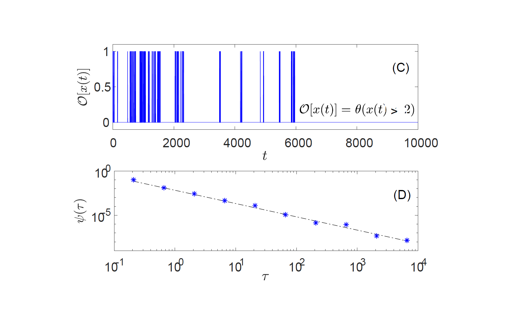
In Fig. 1 we demonstrate the long sojourn times close to zero. We generate a trajectory $x(t)$ from the Langevin equation (1) with (4) and Stratonovich interpretation. We use $\alpha=3/2$ and the measurement time is $10^{4}$. In all simulations in this paper we use $D_{0}=1/2$ and $\ell=1$. $x(t)$ is given in the panel (A). In panel (B) we present the observable ${\cal O}[x(t)]=\theta(0.4<x(t)<0.6)$ where $x(t)$ is the same realization given in (A). In panel (C) we show the mathematical observable ${\cal O}[x(t)]=\sin\left[1/x(t)\right]$, which is chosen to demonstrate the fact that the choice of a specific observable is not important. Both observables [in panels (B) and (C)] are integrable with respect to the infinite density. Therefore, they share a similar property; the observables have long sojourn times close to zero, thus Eq. (27) with $\beta=1/2$ in agreement with Eq. (20) is valid, see Fig. 1.

In Fig. 2 we present the simulation results of $P(x,t)$ for processes $\sqrt{D(x)}=\alpha x^{1-1/\alpha}$ where $\alpha=3/2$. Panel (A) presents the results for Hänggi-Klimontovich interpretation $(A=0)$, panel (B) for Stratonovich ($A=1$), and (C) shows results for Itô interpretation $(A=2)$. The agreement between the simulation results (symbols), the time-dependent solution Eq. (11) (solid lines) and the limit distribution Eq. (15) (dashed lines) is visible. These simulations clearly demonstrate that the nonnormalized state is measurable. Of-course for finite times we see deviations, however as we increase the measurement time, the nonnormalized state is approached.

As explained above, for an observable ${\cal O}[x(t)]$ which is integrable with respect to ${\cal I}_{\infty}(x)$ infinite ergodic theory holds. For the illustration we choose ${\cal O}[x(t)]=\theta(0.4<x(t)<0.6)$ and define the random variable $\xi$ using Eq. (24). Then, in the long time limit, ${\rm P}(\xi)$ follows the Mittag-Leffler distribution of order $\beta$. In Fig. 3 we present the simulation results (with symbols) for the PDF of $\xi$ where $\alpha=1.4$, $t=10^{3}$ and $10^{5}$ particles. Panel (A) presents results for Hänggi-Klimontovich (Mittag-Leffler function of order 0.3), panel (B) presents the results for Stratonovich (Mittag-Leffler of order 0.5) and (C) for Itô interpretation (Mittag-Leffler or order 0.7). Here we demonstrate that the statistics of $\xi$ depends on the stochastic interpretation of the Langevin equation (1).

As was mentioned in the Introduction, we study processes where, in the vicinity of some point $\tilde{x}$, the diffusion coefficient is Eq. (3). In the previous subsections we considered a specific form of $D(x)$, Eq. (4), which allowed us to obtain exact results for any time $t$. Our aim now is to show that the features such as the infinite density are generally valid, in particular for processes with $D(x)\neq 0$ on $x=0$. For example consider a process with

$$\sqrt{D(x)}=\sqrt{2D_{0}}\cdot\begin{cases}1&|x|<x_{c}\\ \alpha\left|\frac{x}{\ell}\right|^{1-1/\alpha}&|x|\geq x_{c}\end{cases}$$

(28)

where $x_{c}=\ell\alpha^{\frac{\alpha}{1-\alpha}}$, so $D(x)$ is continuous. We define the process in $(-\infty,\infty)$. Furthermore, to fulfill the growth condition we demand $\alpha>0$, see [4] and App. A. Here, using the transformation $y(x)\equiv\int_{0}^{x}{\rm d}x^{\prime}D(x)^{-1/2}$, we find

$$\frac{d\sqrt{D(y)}}{dy}\frac{1}{\sqrt{D(y)}}=\begin{cases}0&|y|<y_{c}\\ \frac{-U_{0}}{|y|}&|y|>y_{c},\end{cases}$$

(29)

which is the effective force defined in Eq. (8). The concentration of Brownian particles with the effective force Eq. (29), initially on the origin and $-1<U_{0}<1$, is

$$P(y,t)\approx\begin{cases}\frac{1}{\Gamma\left(\frac{1}{2}-\frac{U_{0}}{2}\right)}|y|^{-U_{0}}(2t)^{\frac{U_{0}}{2}-\frac{1}{2}}e^{-\frac{y^{2}}{2t}}&|y|>y_{c}\\ \frac{1}{\Gamma\left(\frac{1}{2}-\frac{U_{0}}{2}\right)}(y_{c})^{-U_{0}}(2t)^{\frac{U_{0}}{2}-\frac{1}{2}}&|y|<y_{c},\end{cases}$$

(30)

when the long-time limit is taken, see derivation in [43]. Back to $P(x,t)$ we obtain

	$\displaystyle P(x,t)$		$\displaystyle\approx\frac{1}{\Gamma\left[\frac{1-U_{0}}{2}\right]}\frac{\ell^{-U_{0}+\frac{U_{0}}{\alpha}}}{(4D_{0}t)^{({1-U_{0}})/{2}}}\cdot$		(31)
			$\displaystyle\begin{cases}\frac{1}{\alpha}\left|\frac{x}{\ell}\right|^{-1+\frac{1}{\alpha}}|x|^{-\frac{U_{0}}{\alpha}}\exp\left[-\frac{\ell^{2-\frac{2}{\alpha}}x^{\frac{2}{\alpha}}}{4D_{0}t}\right],&|x|\geq x_{c},\\ x_{c}^{-\frac{U_{0}}{\alpha}},&|x|<x_{c}.\end{cases}$

The infinite density, given by the condition $J=0$, is

	$\displaystyle{\cal I}_{\infty}(x)=CD(x)^{-\frac{A}{2}}=$		(32)
	$\displaystyle\frac{C}{(2D_{0})^{A/2}}\begin{cases}|\alpha|^{-A}\left|\frac{x}{\ell}\right|^{A(-1+\frac{1}{\alpha})},&|x|\geq x_{c},\\ 1,&|x|<x_{c}\end{cases}$

so the relation

$$\lim_{t\rightarrow\infty}P(x,t)t^{\frac{\alpha}{2}-\frac{A}{2}(\alpha-1)}={\cal I}_{\infty}(x),$$

(33)

holds, similarly to Eq. (15), with $C=2^{-\alpha(1-A)-\frac{A}{2}}D_{0}^{-{\alpha(1-A)}/{2}}\ell^{-U_{0}}|\alpha|^{A-1}/{\Gamma\left[\frac{1-U_{0}}{2}\right]}$. As was mentioned above, from the existence of a nonnormalizable solution ${\cal I}_{\infty}(x)$ related to $P(x,t)$, as given in (33), one can prove that Eqs. (23) and (27) with $\beta$ given in Eq. (20) still hold, so infinite ergodic theory is valid. The proof and the results are similar to Sec. II.2. From Eq. (32) we see that the nonnormalized state has a structure, which deviates from a pure power law Eq. (14). Generally, since ${\cal I}_{\infty}(x)\propto D(x)^{-A/2}$, the infinite density is specific to the details of the system.

In Eq. (28) we have regularized $D(x)$ in the vicinity of the origin [compare with Eq. (4)], namely $D(x)\neq 0$ when $x\rightarrow 0$. Therefore, when $U_{0}>1$, one finds a normalizable steady state and the process is ergodic, see [43, 8]. The equilibrium distribution is given by

	$\displaystyle P_{\rm eq}(x)=$		(34)
	$\displaystyle\frac{1-U_{0}}{2x_{c}(1-U_{0}-\alpha)}\begin{cases}|\alpha|^{-A}\left|\frac{x}{\ell}\right|^{A(-1+\frac{1}{\alpha})},&|x|\geq x_{c},\\ 1,&|x|<x_{c}\end{cases}$

which is now normalized as usual, i.e. $\int_{-\infty}^{\infty}P_{\rm eq}(x){\rm d}x=1$, and the standard ergodic theory holds. It means that in the long time limit, when ${\cal O}[x(t)]$ is integrable with respect to the equilibrium state, one finds

$${\rm P}(\xi)=\delta(\xi-1),$$

(35)

where here $\xi\equiv\lim_{t\rightarrow\infty}{\overline{\cal O}}/{\langle{\cal O}\rangle}$. Interestingly, this ergodic phase is obtained when using Itô interpretation with $\alpha>2$. For other forms (i.e. Stratonovich or Hänggi-Klimantovich) with $\alpha>0$ the ergodic phase cannot be obtained with Eq. (1). Needless to say that in this case, when adding a binding force to the Langevin equation (1), e.g. an harmonic potential, one may obtain an ergodic phase, with all interpretations.

For simplicity here we consider only the Stratonovich interpretation. The process is bounded in $[0,L]$ and

$$\sqrt{D(x)}=\sqrt{2D_{0}}|\alpha|(x/\ell)^{1-1/\alpha}{\rm\ when\ }0\leq x\leq L$$

(38)

with $\alpha<0$. Clearly as $x\rightarrow 0$ the diffusivity becomes small, and hence intuitively a particle in the vicinity of zero is slowed down. This, in turn, implies a pile up of particles close to zero, which is associated with the non-integrable state. Then the infinite density which, as mentioned, is defined via Eq. (13), is

$${\cal I}_{\infty}(x)=CD(x)^{-1/2}=C\frac{\ell^{1-1/\alpha}}{\sqrt{2D_{0}\alpha^{2}}}x^{-1+1/\alpha},$$

(39)

where $C$ is determined below using the time-dependent solution. Here ${\cal I}_{\infty}(x)$ is nonnormalizable due to its behavior close to zero.

To solve the Fokker-Planck equation (5), we define a new variable

$$y(x)\equiv\int_{x}^{L}\frac{{\rm d}x^{\prime}}{\sqrt{D(x^{\prime})}}=\frac{\ell^{1-1/\alpha}}{\sqrt{2D_{0}}}\left[x^{1/\alpha}-L^{1/\alpha}\right],$$

(40)

then Eq. (5), with $A=1$ (i.e. Stratonovich form), transforms into

$$\frac{\partial}{\partial t}P(y,t)=\frac{1}{2}\frac{\partial^{2}}{\partial y^{2}}P(y,t)$$

(41)

in the interval $y\in[0,\infty)$ with the reflecting boundary condition $\partial_{y}P(y,t)|_{y=0}=0$. Solving Eq. (41) with the method of images, considering the initial condition $y(t)|_{t=0}=y_{0}$, and transforming back to $x$ using Eq. (40), gives

	$\displaystyle P(x,t)=\frac{(x/\ell)^{-1+\frac{1}{\alpha}}}{\sqrt{4D_{0}\pi t}|\alpha|}\left\{\exp\left[-\frac{\left(x^{\frac{1}{\alpha}}-x_{0}^{\frac{1}{\alpha}}\right)^{2}\ell^{2-\frac{2}{\alpha}}}{4D_{0}t}\right]\right.$
	$\displaystyle\left.+\exp\left[-{\frac{\left(x^{\frac{1}{\alpha}}+x_{0}^{\frac{1}{\alpha}}-2L^{\frac{1}{\alpha}}\right)^{2}\ell^{2-\frac{2}{\alpha}}}{4D_{0}t}}\right]\right\}.$		(42)

The following relation between the time-dependent solution $P(x,t)$ and the infinite density in Eq. (39) is fulfilled

$$\lim_{t\rightarrow\infty}t^{1/2}P(x,t)=\sqrt{\frac{1}{\pi D_{0}\alpha^{2}}}(x/\ell)^{-1+1/\alpha}={\cal I}_{\infty}(x),$$

(43)

hence we identify the constant to be $C=(2\pi)^{-1/2}$.

In Fig. 7 we present $t^{1/2}P(x,t)$ versus $x$ for several times. The symbols are the simulation results and the solid curves represent the analytic prediction. The collapse of the data for large $x$ and the approach to ${\cal I}_{\infty}(x)$ while increasing the time are clearly visible.

In the previous example ${\cal I}_{\infty}(x)$ decays as a power law in the whole domain $[0,L]$ peaking on $x=0$. We now consider

	$\displaystyle\sqrt{D(x)}=$		(46)
	$\displaystyle\sqrt{2D_{0}}\left[|\alpha|\left(\frac{x}{\ell}\right)^{1-1/\alpha}\theta(0\leq x\leq x_{c})+\theta(x_{c}<x\leq L)\right]$

where $\alpha$ is negative. $x_{c}$ is chosen so $D(x)$ is continuous. Similar to the previous example, $D(x)$ vanishes when $x\rightarrow 0$, but the field $D(x)$ has some structure. Also here we define $y(x)=\int_{x}^{L}{{\rm d}x^{\prime}}\left[{D(x^{\prime})}\right]^{-1/2}$ and find the time dependent solution

	$\displaystyle P(x,t)=$		$\displaystyle\frac{1}{\sqrt{2\pi tD(x)}}\left\{\exp\left[-\frac{\left(y(x)-y(x_{0})\right)^{2}}{2t}\right]\right.$		(47)
			$\displaystyle\left.+\exp\left[-{\frac{\left(y(x)+y(x_{0})\right)^{2}}{2t}}\right]\right\}.$

The solution obtained from $J=0$, see Eq. (13), is

$${\cal I}_{\infty}(x)=\sqrt{\frac{1}{\pi D_{0}}}\begin{cases}\frac{1}{|\alpha|}\left(\frac{x}{\ell}\right)^{-1+1/\alpha}&0<x<x_{c}\\ 1&x_{c}<x<L\end{cases}$$

(48)

which diverges due to its behavior in $x=0$. Here, $\lim_{t\rightarrow\infty}t^{1/2}P(x,t)={\cal I}_{\infty}(x)$. In Fig. 10 we show $t^{1/2}P(x,t)$ versus $x$ which approaches ${\cal I}_{\infty}(x)$ as we increase $t$. Clearly, it illustrates that the structure of the infinite density ${\cal I}_{\infty}(x)$ depends on $D(x)$.

References

- [1] P. Lançon, G. Batrouni, L. Lobry, and N. Ostrowsky, Euro. Phys. Lett. 54, 28 (2001).
- [2] J. Pešek, P. Baerts, B. Smeets, C. Maes, and H. Ramon, Soft matter 12, 3360 (2016).
- [3] S. Regev, N. Grønbech-Jensen, and O. Farago, Physical Review E 94, 012116 (2016).
- [4] C. W. Gardiner, Handbook of Stochastic Methods for Physics, Chemistry and the Natural Sciences (Springer, 2003).
- [5] C. Cohen-Tannoudji, in Fundamental Systems in Quantum Optics, Les Houches session LIII, edited by J. Dalibard, J. M. Raimond, and J. Zinn-Justin (Elsevier Science, Amsterdam, 1992).
- [6] F. Bardou, J.-P. Bouchaus, A. Aspect, and C. Cohen-Tannoudji, Lévy statistics and laser cooling: how rare events bring atoms to rest (Cambridge University Press, 2002).
- [7] O. Farago and N. Grønbech-Jensen, The Journal of chemical physics 144, 084102 (2016).
- [8] A. Bray, Physical Review E 62, 103 (2000).
- [9] B. Oksendal, Stochastic differential equations: an introduction with applications (Springer Science & Business Media, 2013).
- [10] S. Pieprzyk, D. Heyes, and A. Brańka, Biomicrofluidics 10, 054118 (2016).
- [11] A. M. Berezhkovskii and D. E. Makarov, The Journal of chemical physics 147, 201102 (2017).
- [12] T. Kühn, T. O. Ihalainen, J. Hyväluoma, N. Dross, S. F. Willman, J. Langowski, M. Vihinen-Ranta, and J. Timonen, PLoS One 6, e22962 (2011).
- [13] B. Kaulakys and M. Alaburda, J. Stat. Mech. Theo. Exp p. P02051 (2009).
- [14] K. Itô, Proceedings of the Imperial Academy 20, 519 (1944).
- [15] R. Stratonovich, SIAM Journal on Control 4, 362 (1966).
- [16] P. Hanggi, Physical Review A 25, 1130 (1982).
- [17] Y. L. Klimontovich, Physica A: Statistical Mechanics and its Applications 163, 515 (1990).
- [18] R. Kubo, M. Toda, and N. Hashitsume, Statistical physics II: nonequilibrium statistical mechanics (Springer, 2012).
- [19] E. Wong and M. Zakai, Ann. Math. Stat 36, 1560 (1965).
- [20] G. Volpe and J. Wehr, Rep. Prog. Phys 79, 053901 (2016).
- [21] J. Von Neumann, Invariant measures (American Mathematical Soc., 1991).
- [22] M. Thaler, Israel J. Math 46, 67 (1983).
- [23] M. Thaler and R. Zweimüller, Probab. Theory Related Fields 135, 15 (2006).
- [24] N. Korabel and E. Barkai, Phys. Rev. Lett. 102, 050601 (2009).
- [25] T. Akimoto and T. Miyaguchi, Physical Review E 82, 030102(R) (2010).
- [26] D. A. Kessler and E. Barkai, Phys. Rev. Lett 105, 120602 (2010).
- [27] A. Rebenshtok, S. Denisov, P. Hänggi, and E. Barkai, Phys. Rev. E 90, 062135 (2014).
- [28] E. Aghion, D. A. Kessler, and E. Barkai, arXiv preprint arXiv:1804.05571 (2018).
- [29] J. Aaronson, An introduction to infinite ergodic theory, 50 (American Mathematical Soc., 1997).
- [30] J. Aaronson, M. Thaler, and R. Zweimüller, Ergodic Theory and Dynamical Systems 25, 959 (2005).
- [31] L. F. Richardson, Proc. R. Soc. Lond. A 110, 709 (1926).
- [32] G. Biroli, G. Bunin, and C. Cammarota, arXiv preprint arXiv:1710.03606 (2017).
- [33] A. G. Cherstvy, A. V. Chechkin, and R. Metzler, New J. Phys. 15, 083039 (2013).
- [34] A. G. Cherstvy and R. Metzler, Phys. Chem. Chem. Phys. 15, 20220 (2013).
- [35] A. G. Cherstvy and R. Metzler, Phys. Rev. E 90, 012134 (2014).
- [36] A. G. Cherstvy and R. Metzler, J. Stat. Mech: Theo. Exp. 2015, P05010 (2015).
- [37] B. O’Shaughnessy and I. Procaccia, Physical Review Letters 54, 455 (1985).
- [38] S. Havlin and D. Ben-Avraham, Advances in Physics 36, 695 (1987).
- [39] E. Martin, U. Behn, and G. Germano, Physical Review E 83, 051115 (2011).
- [40] S. Redner, A guide to first-passage processes (Cambridge University Press, 2001).
- [41] C. Godreche and J. Luck, J. Stat. Phys. 104, 489 (2001).
- [42] R. Metzler, J.-H. Jeon, A. G. Cherstvy, and E. Barkai, Physical Chemistry Chemical Physics 16, 24128 (2014).
- [43] A. Dechant, E. Lutz, E. Barkai, and D. Kessler, Journal of Statistical Physics 145, 1524 (2011).
- [44] G. Margolin and E. Barkai, J. Stat. Phys. 122, 137 (2006).
- [45] T. Akimoto, Journal of Statistical Physics 132, 171 (2008).
- [46] W. Feller, An Introduction to Probability Theory and Its Applications (1965).
- [47] T. Akimoto and E. Barkai, Phys. Rev. E 87, 032915 (2013).