跳到论文正文
W Papers独立论文阅读器 arXiv:1808.02419 论文正文 计算阅读时间 · 0%
引用这篇论文根据当前论文元数据生成,正式投稿前建议核对。


License: arXiv.org perpetual non-exclusive license
arXiv:1808.02419v3 [math-ph] 22 Aug 2018

The largest real eigenvalue in the real Ginibre ensemble and its relation to the Zakharov-Shabat systemThanks: T.B. acknowledges support of the AMS and the Simons Foundation through a travel grant and is grateful to B. Rider, P. Deift, and P. Miller for stimulating discussions about this project. J.B. is supported by the NSF grant DMS-1664692. Both authors initiated this work during the 2017 PCMI summer session on random matrices, funded in part by the NSF grant DMS-1441467. The authors would also like to thank P. Forrester for bringing [19] to their attention.

Jinho Baik Address: Department of Mathematics, University of Michigan, 2074 East Hall, 530 Church Street, Ann Arbor, MI 48109-1043, United States Email address: baik@umich.edu and Thomas Bothner Address: Department of Mathematics, University of Michigan, 2074 East Hall, 530 Church Street, Ann Arbor, MI 48109-1043, United States Email address: bothner@umich.edu
Date: August 24, 2026
Abstract.

The real Ginibre ensemble consists of n×nn\times n real matrices 𝐗{\bf X} whose entries are i.i.d. standard normal random variables. In sharp contrast to the complex and quaternion Ginibre ensemble, real eigenvalues in the real Ginibre ensemble attain positive likelihood. In turn, the spectral radius Rn=max1≤j≤n⁡|zj​(𝐗)|R_{n}=\max_{1\leq j\leq n}|z_{j}({\bf X})| of the eigenvalues zj​(𝐗)∈ℂz_{j}({\bf X})\in\mathbb{C} of a real Ginibre matrix 𝐗{\bf X} follows a different limiting law (as n→∞n\rightarrow\infty) for zj​(𝐗)∈ℝz_{j}({\bf X})\in\mathbb{R} than for zj​(𝐗)∈ℂ∖ℝz_{j}({\bf X})\in\mathbb{C}\setminus\mathbb{R}. Building on previous work by Rider, Sinclair [26] and Poplavskyi, Tribe, Zaboronski [25], we show that the limiting distribution of maxj:zj∈ℝzj(𝐗)\max_{j:z_{j}\in\mathbb{R}}z_{j}({\bf X}) admits a closed form expression in terms of a distinguished solution to an inverse scattering problem for the Zakharov-Shabat system. As byproducts of our analysis we also obtain a new determinantal representation for the limiting distribution of maxj:zj∈ℝzj(𝐗)\max_{j:z_{j}\in\mathbb{R}}z_{j}({\bf X}) and extend recent tail estimates in [25] via nonlinear steepest descent techniques.

Key words and phrases: 
Real Ginibre ensemble, extreme value statistics, Riemann-Hilbert problem, Zakharov-Shabat system, inverse scattering theory, Deift-Zhou nonlinear steepest descent method.
2010 Mathematics Subject Classification
Primary 60B20; Secondary 45M05, 60G70.

1. Introduction and statement of results

This paper is foremost concerned with the derivation of an integrable system for the limiting distribution function

limn→∞ℙ(maxj:zj∈ℝzj(𝐗)≤n+t),t∈ℝ,\lim_{n\rightarrow\infty}\mathbb{P}\left(\max_{j:z_{j}\in\mathbb{R}}z_{j}({\bf X})\leq\sqrt{n}+t\right),\ \ \ \ t\in\mathbb{R},

of the largest real eigenvalue of a random matrix 𝐗∈ℝn×n{\bf X}\in\mathbb{R}^{n\times n} chosen from the real Ginibre ensemble.

Definition 1.1 (Ginibre [21], 1965).

A random matrix 𝐗∈ℝn×n{\bf X}\in\mathbb{R}^{n\times n} is said to belong to the real Ginibre ensemble (GinOE) if its entries are independently chosen with pdf’s

12​π​e−12​xj​k2, 1≤j,k≤n.\frac{1}{\sqrt{2\pi}}\mathrm{e}^{-\frac{1}{2}x_{jk}^{2}},\ \ \ \ 1\leq j,k\leq n.

Equivalently, the joint pdf of all the independent entries equals

f(𝐗)=∏1≤j,k≤n12​πe−12​xj​k2=(2π)−12​n2e−12∑j,k=1nxj​k2=(2π)−12​n2e−12​tr​(𝐗𝐗⊺).f({\bf X})=\prod_{1\leq j,k\leq n}\frac{1}{\sqrt{2\pi}}\mathrm{e}^{-\frac{1}{2}x_{jk}^{2}}=(2\pi)^{-\frac{1}{2}n^{2}}\mathrm{e}^{-\frac{1}{2}\sum_{j,k=1}^{n}x_{jk}^{2}}=(2\pi)^{-\frac{1}{2}n^{2}}\mathrm{e}^{-\frac{1}{2}\textnormal{tr}({\bf X}{\bf X}^{\intercal})}.

The GinOE displays certain similarities to the classical Gaussian Orthogonal Ensemble (GOE) but the presence of, both, real and complex eigenvalues introduces also new phenomena. For instance, on a global scale, Wigner’s semicircle law in the GOE is replaced by the following circular law [14]: let

μ𝐗(s,t)=1n#{1≤j≤n:ℜzj(𝐗)≤s,ℑzj(𝐗)≤t},s,t∈ℝ\mu_{\bf X}(s,t)=\frac{1}{n}\#\big\{1\leq j\leq n:\ \Re z_{j}({\bf X})\leq s,\ \Im z_{j}({\bf X})\leq t\big\},\ \ \ s,t\in\mathbb{R}

denote the empirical spectral distribution of the eigenvalues {zj​(𝐗)}j=1n\{z_{j}({\bf X})\}_{j=1}^{n} of a matrix 𝐗∈GinOE{\bf X}\in\textnormal{GinOE}, then the random measure μ𝐗/n\mu_{\bf X}/\sqrt{n} converges almost surely (as n→∞n\rightarrow\infty) to the uniform distribution on the unit disk, see Figure 1 below.

Remark 1.2.

The circular law is a universal limiting law: it holds true for any n×nn\times n random matrix 𝐗{\bf X} whose entries are i.i.d. complex random variables with mean zero and variance one, see [29] and references therein to the long and rich history of the circular law.

Refer to caption
Refer to caption
Figure 1. The circular law for 10001000 real (rescaled) Ginibre matrices of varying dimensions n×nn\times n in comparison with the unit circle boundary. We plot n=2,4,8,16n=2,4,8,16 from left to right. A saturn effect is clearly visible on the real line.

On a local scale, Figure 1 indicates that fluctuations of the spectral radius Rn=max1≤j≤n⁡|zj​(𝐗)|R_{n}=\max_{1\leq j\leq n}|z_{j}({\bf X})| around n\sqrt{n} behave differently depending on whether zj∈ℝz_{j}\in\mathbb{R} or zj∈ℂ∖ℝz_{j}\in\mathbb{C}\setminus\mathbb{R}. And indeed, the above-mentioned saturn effect was quantified recently and the following central limit theorem derived.

Theorem 1.3 (Rider, Sinclair [26], 2014; Poplavskyi, Tribe, Zaboronski [25], 2017).

Let {zj​(𝐗)}j=1n\{z_{j}({\bf X})\}_{j=1}^{n} denote the eigenvalues of a n×nn\times n random matrix 𝐗∈GinOE{\bf X}\in\textnormal{GinOE}. Then,

limn→∞ℙ(maxj:zj∈ℂ∖ℝ|zj(𝐗)|≤n+γn4+t4​γn)=e−12​e−t,t∈ℝ\lim_{n\rightarrow\infty}\mathbb{P}\left(\max_{j:z_{j}\in\mathbb{C}\setminus\mathbb{R}}|z_{j}({\bf X})|\leq\sqrt{n}+\sqrt{\frac{\gamma_{n}}{4}}+\frac{t}{\sqrt{4\gamma_{n}}}\right)=\mathrm{e}^{-\frac{1}{2}\mathrm{e}^{-t}},\ \ \ \ t\in\mathbb{R}

with γn=ln⁡(n/(2​π​(ln⁡n)2))\gamma_{n}=\ln(n/(2\pi(\ln n)^{2})). In addition,

limn→∞ℙ(maxj:zj∈ℝzj(𝐗)≤n+t)=det(1−Tχt↾L2​(ℝ))Γt,t∈ℝ,\lim_{n\rightarrow\infty}\mathbb{P}\left(\max_{j:z_{j}\in\mathbb{R}}z_{j}({\bf X})\leq\sqrt{n}+t\right)=\sqrt{\det(1-T\chi_{t}\upharpoonright_{L^{2}(\mathbb{R})})\Gamma_{t}},\ \ \ \ \ t\in\mathbb{R}, (1.1)

where χt\chi_{t} is the operator of multiplication by χ(t,+∞)​(x)\chi_{(t,+\infty)}(x), the characteristic function of (t,+∞)⊂ℝ(t,+\infty)\subset\mathbb{R}, and T:L2​(ℝ)→L2​(ℝ)T:L^{2}(\mathbb{R})\rightarrow L^{2}(\mathbb{R}) the trace-class integral operator with kernel

T⁡(x,y)=1π​∫0∞e−(x+u)2​e−(y+u)2​𝑑u.T(x,y)=\frac{1}{\pi}\int_{0}^{\infty}\mathrm{e}^{-(x+u)^{2}}\mathrm{e}^{-(y+u)^{2}}\,{\mathrm{d}}u. (1.2)

Moreover,

Γt=1−∫t∞G(x)((1−Tχt↾L2​(ℝ))−1g)(x)dx\Gamma_{t}=1-\int_{t}^{\infty}G(x)\big((1-T\chi_{t}\upharpoonright_{L^{2}(\mathbb{R})})^{-1}g\big)(x)\,{\mathrm{d}}x (1.3)

with g⁡(x)=1π​e−x2g(x)=\frac{1}{\sqrt{\pi}}\mathrm{e}^{-x^{2}} and G⁡(x)=∫−∞xg⁡(y)​𝑑yG(x)=\int_{-\infty}^{x}g(y)\,{\mathrm{d}}y.

When compared to the GOE, (1.1) plays the analogue of the celebrated Tracy-Widom edge law for the largest eigenvalue λmax\lambda_{\max}, cf. [31]. Indeed we recall that in the GOE, as n→∞n\rightarrow\infty,

λmax⇒2​n+12​n16​F1,\lambda_{\max}\Rightarrow\sqrt{2n}+\frac{1}{\sqrt{2}\,n^{\frac{1}{6}}}F_{1},

with the cdf

F1​(t)=det(1−Kχt↾L2​(ℝ))Γ^t,t∈ℝ,F_{1}(t)=\sqrt{\det(1-K\chi_{t}\upharpoonright_{L^{2}(\mathbb{R})})\widehat{\Gamma}_{t}},\ \ \ \ \ t\in\mathbb{R}, (1.4)

where K:L2​(ℝ)→L2​(ℝ)K:L^{2}(\mathbb{R})\rightarrow L^{2}(\mathbb{R}) is the integral operator with Airy kernel K⁡(x,y)=∫0∞Ai​(x+u)​Ai​(y+u)​𝑑uK(x,y)=\int_{0}^{\infty}\textnormal{Ai}(x+u)\textnormal{Ai}(y+u)\,{\mathrm{d}}u in terms of the Airy function Ai​(z)\textnormal{Ai}(z), [24]. Moreover, see e.g. [18, Section 9.79.7],

Γ^t=1−∫t∞A(x)((1−Kχt↾L2​(ℝ))−1Ai)(x)dx;A(x)=∫−∞xAi(y)dy.\widehat{\Gamma}_{t}=1-\int_{t}^{\infty}A(x)\big((1-K\chi_{t}\upharpoonright_{L^{2}(\mathbb{R})})^{-1}\textnormal{Ai}\big)(x)\,{\mathrm{d}}x;\ \ \ \ \ \ \ A(x)=\int_{-\infty}^{x}\textnormal{Ai}(y)\,{\mathrm{d}}y. (1.5)

1.1. An integrable system for (1.1)

The formal similarities between (1.4), (1.5) and (1.1), (1.3) are quite obvious, still while the operator KK is of integrable type in the sense of [23], i.e. has a kernel of the form

K⁡(x,y)=𝐟⊺​(x)​𝐠​(y)x−y,𝐟⁡(z)=[Ai​(z)−Ai′​(z)],𝐠⁡(z)=[Ai′​(z)Ai​(z)],K(x,y)=\frac{{\bf f}^{\intercal}(x){\bf g}(y)}{x-y},\ \ \ \ {\bf f}(z)=\begin{bmatrix}\textnormal{Ai}(z)\\ -\textnormal{Ai}^{\prime}(z)\end{bmatrix},\ \ \ {\bf g}(z)=\begin{bmatrix}\textnormal{Ai}^{\prime}(z)\\ \textnormal{Ai}(z)\end{bmatrix}, (1.6)

this is not true for TT with kernel (1.2), see explicitly [26, Section 4]. For this reason neither the standard Tracy-Widom method [30] used in the derivation of an integrable system (a.k.a. a closed form expression) for the limiting distribution function (1.1) nor the Riemann-Hilbert problem based techniques of Borodin and Deift [9] are directly applicable. However, as we will show below, the situation with (1.2) is not too bad, since the operator T​χtT\chi_{t} is of integrable type up to Fourier conjugation, see Proposition 3.3 below. This observation combined with certain additional manipulations for the Fredholm determinant and the factor Γt\Gamma_{t} in (1.1), see Sections 2, 3 and 4 below, yields an explicit integrable system for F⁡(t)F(t) and a subsequent closed form, Tracy-Widom like, formula. In fact we shall state the sought after closed form expression for the following generalization of (1.1) that contains a generating function parameter γ∈[0,1]\gamma\in[0,1],

F(t;γ):=det(1−γTχt↾L2​(ℝ))Γt​γ,withΓt​γ:=1−γ∫t∞G(x)((1−γTχt↾L2​(ℝ))−1g)(x)dx.F(t;\gamma):=\sqrt{\det(1-\gamma T\chi_{t}\upharpoonright_{L^{2}(\mathbb{R})})\Gamma_{t\gamma}},\ \ \textnormal{with}\ \ \Gamma_{t\gamma}:=1-\gamma\int_{t}^{\infty}G(x)\big((1-\gamma T\chi_{t}\upharpoonright_{L^{2}(\mathbb{R})})^{-1}g\big)(x)\,{\mathrm{d}}x. (1.7)

The main result of our paper, see Theorem 1.5 below, is a closed form expression for F⁡(t,γ)F(t;\gamma) in terms of a distinguished solution to an inverse scattering problem for the Zakharov-Shabat (ZS) system [32, 1]. As it is standard in scattering theory, we shall formulate this inverse problem as a Riemann-Hilbert problem (RHP):

Riemann-Hilbert Problem 1.4.

For any (x,γ)∈ℝ×[0,1](x,\gamma)\in\mathbb{R}\times[0,1], determine 𝐗⁡(z)=𝐗⁡(z,x,γ)∈ℂ2×2{\bf X}(z)={\bf X}(z;x,\gamma)\in\mathbb{C}^{2\times 2} such that

  1. (1)

    𝐗⁡(z){\bf X}(z) is analytic for z∈ℂ∖ℝz\in\mathbb{C}\setminus\mathbb{R} and has a continuous extension on the closed upper and lower half-planes.

  2. (2)

    The limiting values 𝐗±​(z)=limϵ↓0𝐗⁡(z±i​ϵ),z∈ℝ{\bf X}_{\pm}(z)=\lim_{\epsilon\downarrow 0}{\bf X}(z\pm\mathrm{i}\epsilon),z\in\mathbb{R} satisfy the jump condition

    𝐗+(z)=𝐗−(z)[1−|r⁡(z)|2−r¯​(z)​e−2​i​x​zr⁡(z)​e2​i​x​z1],z∈ℝwithr(z)=r(z;γ)=−iγe−14​z2.{\bf X}_{+}(z)={\bf X}_{-}(z)\begin{bmatrix}1-|r(z)|^{2}&-\bar{r}(z)\mathrm{e}^{-2\mathrm{i}xz}\vskip 3.0pt plus 1.0pt minus 1.0pt\\ r(z)\mathrm{e}^{2\mathrm{i}xz}&1\end{bmatrix},\ \ z\in\mathbb{R}\ \ \ \ \ \textnormal{with}\ \ \ r(z)=r(z;\gamma)=-\mathrm{i}\sqrt{\gamma}\,\mathrm{e}^{-\frac{1}{4}z^{2}}. (1.8)
  3. (3)

    As z→∞z\rightarrow\infty, we require the normalization

    𝐗⁡(z)=𝕀+𝐗1​z−1+𝐗2​z−2+𝒪⁡(z−3);𝐗i=𝐗i​(x,γ)=[Xij​k​(x,γ)]j,k=12.{\bf X}(z)=\mathbb{I}+{\bf X}_{1}z^{-1}+{\bf X}_{2}z^{-2}+\mathcal{O}\big(z^{-3}\big);\ \ \ \ \ {\bf X}_{i}={\bf X}_{i}(x,\gamma)=\big[X_{i}^{jk}(x,\gamma)\big]_{j,k=1}^{2}.

Note that r⁡(z,γ)∈𝒮⁡(ℝ)r(z;\gamma)\in\mathcal{S}(\mathbb{R}), the Schwartz space on the line, but ‖r‖∞=supz∈ℝ|r⁡(z)|<1\|r\|_{\infty}=\sup_{z\in\mathbb{R}}|r(z)|<1 only for γ∈[0,1)\gamma\in[0,1). Hence r⁡(z,γ)r(z;\gamma), the so-called reflection coefficient, does not belong to the standard Beals-Coifman class of reflection coefficients, cf. [3, 4], in the case (1.1) most relevant to the GinOE. For this reason we will prove unique solvability of RHP 1.4 for all (x,γ)∈ℝ×[0,1](x,\gamma)\in\mathbb{R}\times[0,1] and thus also existence of the coefficients 𝐗i​(x,γ){\bf X}_{i}(x,\gamma) directly in the sections below. We now present our main result.

Theorem 1.5.

For any (t,γ)∈ℝ×[0,1](t,\gamma)\in\mathbb{R}\times[0,1],

(F(t;γ))2=exp[−14∫t∞(x−t)|y(x2;γ)|2dx]{coshμ(t;γ)−γsinhμ(t;γ)},\big(F(t;\gamma)\big)^{2}=\exp\bigg[-\frac{1}{4}\int_{t}^{\infty}(x-t)\left|y\left(\frac{x}{2};\gamma\right)\right|^{2}{\mathrm{d}}x\bigg]\bigg\{\cosh\mu(t;\gamma)-\sqrt{\gamma}\sinh\mu(t;\gamma)\bigg\}, (1.9)

using the abbreviation

μ(t;γ):=−i2∫t∞y(x2;γ)dx,\mu(t;\gamma):=-\frac{\mathrm{i}}{2}\int_{t}^{\infty}y\left(\frac{x}{2};\gamma\right)\,{\mathrm{d}}x,

and where y=y⁡(x,γ):ℝ×[0,1]→i​ℝy=y(x;\gamma):\mathbb{R}\times[0,1]\rightarrow\mathrm{i}\mathbb{R} equals y⁡(x,γ):=2​i​X112​(x,γ)y(x;\gamma):=2\mathrm{i}X_{1}^{12}(x,\gamma) in terms of the matrix coefficient 𝐗1​(x,γ){\bf X}_{1}(x,\gamma) in condition (3) of RHP 1.4 above.

Identity (1.9) is the analogue of the Tracy-Widom Painlevé-II formula for F1​(t)F_{1}(t) in case γ=1\gamma=1, see [31]. For γ∈[0,1)\gamma\in[0,1), our definition (1.7) is motivated by the generating function of the soft-edge scaled (t,+∞)(t,+\infty) gap probabilities for the superimposed, cf. [18, Section 6.66.6], orthogonal ensemble

odd​(OEn​(e−x2)∪OEn​(e−x2)).\textnormal{odd}\big(\textnormal{OE}_{n}(\mathrm{e}^{-x^{2}})\cup\textnormal{OE}_{n}(\mathrm{e}^{-x^{2}})\big).

In this context, (1.9) is the direct analogue of [18, (9.150)(9.150)], modulo the replacement of the Painlevé-II transcendent with the above solution entry y⁡(x,γ)y(x;\gamma) of RHP 1.4.

Remark 1.6.

Another possible motivation for the introduction of γ\gamma in (1.7) could arise from studying a thinned version of the real eigenvalues in the GinOE, i.e. from analyzing the point process

𝔛γ={zjγ​(𝐗):zjγ​(𝐗)∈ℝ}j=1n⁡(γ), 1≤n⁡(γ)≤n,\mathfrak{X}^{\gamma}=\{z_{j}^{\gamma}({\bf X}):z_{j}^{\gamma}({\bf X})\in\mathbb{R}\}_{j=1}^{n(\gamma)},\ \ \ 1\leq n(\gamma)\leq n,

obtained from 𝔛={zj(𝐗)∈ℝ}j=1n\mathfrak{X}=\{z_{j}({\bf X})\in\mathbb{R}\}_{j=1}^{n} with 𝐗∈GinOE{\bf X}\in\textnormal{GinOE} by independently removing each real eigenvalue with likelihood γ∈[0,1]\gamma\in[0,1]. For GOE, the largest eigenvalue distribution function after thinning admits a Painlevé closed form expression, see [10, (1.6)(1.6)], in case of GinOE the corresponding result is unknown. It is also not immediately clear whether (1.7) has a probabilistic interpretation in the thinned superimposed orthogonal ensemble. We plan to address this question in a future publication.

Remark 1.7.

We prove existence of y⁡(x,γ)y(x;\gamma) for (x,γ)∈ℝ×[0,1](x,\gamma)\in\mathbb{R}\times[0,1] in Theorem 3.9 and continuity of y⁡(x,γ),x∈ℝy(x;\gamma),x\in\mathbb{R} for any fixed γ∈[0,1]\gamma\in[0,1] in Lemma 2.1 and Corollary 3.6. Moreover we show that y⁡(x,γ)y(x;\gamma) for (x,γ)∈ℝ×[0,1](x,\gamma)\in\mathbb{R}\times[0,1] is purely imaginary and

y⁡(x,γ)=2​i​γπ​e−4​x2​(1+𝒪⁡(e−4​x2)),x→+∞,y(x;\gamma)=2\mathrm{i}\sqrt{\frac{\gamma}{\pi}}\,\mathrm{e}^{-4x^{2}}\left(1+\mathcal{O}\left(\mathrm{e}^{-4x^{2}}\right)\right),\ \ \ x\rightarrow+\infty, (1.10)

i.e. the right-hand side in (1.9) is well-defined.

Returning to the afore-mentioned comparison between GinOE and GOE we see from (1.9) and [31, (53)(53)] that, overall, the main difference in GinOE arises from the presence of the inverse scattering type RHP 1.4 and its solution entry y⁡(x,γ)y(x;\gamma) instead of the more common Painlevé transcendents in the Gaussian invariant ensembles. For this reason we shall briefly review a few selected aspects of the integrability theory of RHP 1.4, see [1, 3, 4, 32] for more details.

1.2. The Zakharov-Shabat system in a nutshell

Note that

𝚿⁡(z):=𝐗⁡(z)​e−i​x​z​σ3,z∈ℂ∖ℝ{\bf\Psi}(z):={\bf X}(z)\mathrm{e}^{-\mathrm{i}xz\sigma_{3}},\ \ \ z\in\mathbb{C}\setminus\mathbb{R}

solves a RHP with an xx-independent jump on ℝ\mathbb{R}, thus ∂𝚿∂x​𝚿−1\frac{\partial{\bf\Psi}}{\partial x}{\bf\Psi}^{-1} is an entire function. In fact, using condition (3) in RHP 1.4 and Liouville’s theorem, we find

∂𝚿∂x={−i​z​σ3+2​i​[0X112−X1210]}​𝚿.\frac{\partial{\bf\Psi}}{\partial x}=\left\{-\mathrm{i}z\sigma_{3}+2\mathrm{i}\begin{bmatrix}0&X_{1}^{12}\vskip 3.0pt plus 1.0pt minus 1.0pt\\ -X_{1}^{21}&0\end{bmatrix}\right\}{\bf\Psi}. (1.11)

But since RHP 1.4 enjoys the symmetry

𝐗⁡(z,x,γ)=σ1​𝐗⁡(z¯,x,γ)¯​σ1,z∈ℂ∖ℝ;σ1=[0110],{\bf X}(z;x,\gamma)=\sigma_{1}\overline{{\bf X}(\bar{z};x,\gamma)}\sigma_{1},\ \ \ \ z\in\mathbb{C}\setminus\mathbb{R};\ \ \ \ \sigma_{1}=\begin{bmatrix}0&1\\ 1&0\end{bmatrix}, (1.12)

we learn that Xi11​(x,γ)=Xi22​(x,γ)¯X_{i}^{11}(x,\gamma)=\overline{X_{i}^{22}(x,\gamma)} as well as Xi21​(x,γ)=Xi12​(x,γ)¯X_{i}^{21}(x,\gamma)=\overline{X_{i}^{12}(x,\gamma)} and thus with y=2​i​X112y=2\mathrm{i}X_{1}^{12} from (1.11),

∂𝚿∂x={−i​z​σ3+[0yy¯0]}​𝚿≡𝐔⁡(z,x,γ)​𝚿.\frac{\partial{\bf\Psi}}{\partial x}=\left\{-\mathrm{i}z\sigma_{3}+\begin{bmatrix}0&y\\ \bar{y}&0\end{bmatrix}\right\}{\bf\Psi}\equiv{\bf U}(z;x,\gamma){\bf\Psi}. (1.13)

This celebrated first order system, known as ZS-system, is directly related to several of the most interesting nonlinear evolution equations in 1+11+1 dimensions which are solvable by the inverse scattering method. For instance, in order to solve the Cauchy problem for the defocusing nonlinear Schrödinger equation,

i​yt+yx​x−2​|y|2​y=0,y⁡(x,0)=y0​(x)∈𝒮⁡(ℝ);y=y⁡(x,t):ℝ2→ℂ,\mathrm{i}y_{t}+y_{xx}-2|y|^{2}y=0,\ \ \ \ y(x,0)=y_{0}(x)\in\mathcal{S}(\mathbb{R});\ \ \ \ \ y=y(x,t):\mathbb{R}^{2}\rightarrow\mathbb{C}, (1.14)

one first computes the reflection coefficient r⁡(z)∈𝒮⁡(ℝ)r(z)\in\mathcal{S}(\mathbb{R}) associated to the initial data y0y_{0} through the direct scattering transform. A basic fact of the scattering theory for the Zhakarov-Shabat system (1.13) states that this transform, i.e. the map y0→ry_{0}\rightarrow r, is a bijection from 𝒮⁡(ℝ)\mathcal{S}(\mathbb{R}) onto 𝒮⁡(ℝ)∩{r:‖r‖∞=supz∈ℝ|r⁡(z)|<1}\mathcal{S}(\mathbb{R})\cap\{r:\,\|r\|_{\infty}=\sup_{z\in\mathbb{R}}|r(z)|<1\}, cf. [3]. Second, one considers RHP 1.4 above subject to the replacement

e2​i​x​z→e2​i​(2​t​z2+x​z),t∈ℝ,\mathrm{e}^{2\mathrm{i}xz}\rightarrow\mathrm{e}^{2\mathrm{i}(2tz^{2}+xz)},\ \ \ t\in\mathbb{R},

and provided this problem is solvable, its (unique) solution in turn leads to a solution of (1.14) with y​(x,0)=y0​(x)y(x,0)=y_{0}(x) via the formula y⁡(x,t)=2​i​X112​(x,t)y(x,t)=2\mathrm{i}X_{1}^{12}(x,t). Thus, in order to solve (1.14), one must solve the tt-modified RHP 1.4 (a.k.a. the inverse scattering transform) for the given reflection coefficient r⁡(z)r(z), determined under the aforementioned bijection y0→ry_{0}\rightarrow r. Returning now to our context, we see that (1.9) therefore depends on a distinguished solution y⁡(x,γ)y(x;\gamma) of the inverse scattering transform for the Zakharov-Shabat system (1.13) subject to the reflection coefficient r⁡(z,γ)=−i​γ​e−14​z2r(z;\gamma)=-\mathrm{i}\sqrt{\gamma}\,\mathrm{e}^{-\frac{1}{4}z^{2}}.

Remark 1.8.

As outlined above, the operator T​χtT\chi_{t} is of integrable type once viewed in Fourier space. This idea was first used in the analysis of single- and multi-time processes in [5, 6]. Specifically, loc. cit. showed that certain matrix Fredholm determinants are expressible as determinants of integrable matrix kernels and thus connected to RHPs. As a direct application of this technique, Bertola and Cafasso re-derived for instance the Adler-van Moerbeke PDE for the joint distributions of the Airy-22 process by Riemann-Hilbert techniques. Our approach to the GinOE and (1.7) is clearly inspired by these works.

1.3. Tail asymptotics

The advantage of the exact formula (1.9) lies in the fact that y=y⁡(x,γ)y=y(x;\gamma) admits a Riemann-Hilbert formulation as outlined in RHP 1.4. Thus its large space/long time behavior can be systematically computed via nonlinear steepest descent techniques [13] and this paths the way to large tail estimates for (1.7). We summarize our second result.

Corollary 1.9.

Let γ∈[0,1]\gamma\in[0,1] and F⁡(t,γ)F(t;\gamma) be defined as in (1.7). Then, as t→+∞t\rightarrow+\infty,

F⁡(t,γ)=1−γ4​erfc​(t)+𝒪⁡(γ32​t−1​e−2​t2),F(t;\gamma)=1-\frac{\gamma}{4}\textnormal{erfc}(t)+\mathcal{O}\left(\gamma^{\frac{3}{2}}t^{-1}\mathrm{e}^{-2t^{2}}\right), (1.15)

in terms of the complementary error function erfc​(z)\textnormal{erfc}(z), cf. [24, 7.2.27.2.2]. On the other hand, as t→−∞t\rightarrow-\infty,

F⁡(t,γ)=eη1​(γ)​t​η0​(γ)​(1+o⁡(1)),η1​(γ)=12​2​π​Li32​(γ),F(t;\gamma)=\mathrm{e}^{\eta_{1}(\gamma)t}\eta_{0}(\gamma)\big(1+o(1)\big),\ \ \ \eta_{1}(\gamma)=\frac{1}{2\sqrt{2\pi}}\,\textnormal{Li}_{\frac{3}{2}}(\gamma), (1.16)

in terms of the polylogarithm Lis​(z)\textnormal{Li}_{s}(z), cf. [24, 25.12.1025.12.10], and with a tt-independent positive factor η0​(γ)\eta_{0}(\gamma).

Estimate (1.15) for γ=1\gamma=1 is standard and known from [20], say. The leading order in (1.14) for γ=1\gamma=1 was obtained by Forrester [19] and also by Poplavskyi, Tribe and Zaboronski [25] using an interesting connection to coalescence processes. Here we employ nonlinear steepest descent techniques to confirm (1.15) for all γ∈[0,1]\gamma\in[0,1] and derive (1.16) for γ∈[0,1)\gamma\in[0,1).

The paper [19] also discusses the thinned version of the real eigenvalues, or equivalently, the generating function for the probability of the number of eigenvalues. Namely, the discussions in the third paragraph of [19, Section 44] claim a leading order term which, after evaluating the integral [19, (4.1)(4.1)] explicitly, is the same as our η1​(γ)\eta_{1}(\gamma) with γ=2​ξ−ξ2\gamma=2\xi-\xi^{2} where 1−ξ1-\xi denotes the removal probability of an eigenvalue. As mentioned above in Remark 1.6 it is interesting to consider the relationship between our F⁡(t,γ)F(t;\gamma) and the thinned version.

Remark 1.10.

As can be seen from (1.16), the left tails of F⁡(t,γ)F(t;\gamma) in the leading order decay to zero exponentially fast for all γ∈(0,1]\gamma\in(0,1]. This is in sharp contrast to the GOE where ln⁡F1​(t)∼124​t3\ln F_{1}(t)\sim\frac{1}{24}t^{3} as t→−∞t\rightarrow-\infty and ln⁡F1​(t,γ)∼−2​v3​π​(−t)3/2\ln F_{1}(t;\gamma)\sim-\frac{2v}{3\pi}(-t)^{3/2} for γ∈(0,1)\gamma\in(0,1) fixed with v=−ln⁡(1−γ)<+∞v=-\ln(1-\gamma)<+\infty, cf. [10]. This means that the large negative xx behavior of ℑ⁡(y⁡(x2,γ))\Im(y(\frac{x}{2};\gamma)) cannot be as sensitive to a small change in γ∈(0,1]\gamma\in(0,1] near γ=1\gamma=1 as the corresponding behavior for the Painlevé-II transcendent u⁡(x,γ)u(x;\gamma), see Figure 4 below for a visualization.

1.4. Numerical comparison

The closed form expression (1.9) is not as optimal for numerical purposes as a single Fredholm determinant formula, compare the discussions in [8]. For this reason we derive a new determinantal formula for the limiting distribution of maxj:zj∈ℝzj(𝐗)\max_{j:z_{j}\in\mathbb{R}}z_{j}({\bf X}) in our third result below. This identity is completely analogous to the Ferrari-Spohn formula [15] in the GOE.

Theorem 1.11.

Let F⁡(t)F(t) be defined as in (1.1). Then

F(t)=det(1−Sχt↾L2​(ℝ)),F(t)=\det(1-S\chi_{t}\upharpoonright_{L^{2}(\mathbb{R})}), (1.17)

where S:L2​(ℝ)→L2​(ℝ)S:L^{2}(\mathbb{R})\rightarrow L^{2}(\mathbb{R}) is the integral operator with kernel

S⁡(x,y)=12​π​e−14​(x+y)2.S(x,y)=\frac{1}{2\sqrt{\pi}}\mathrm{e}^{-\frac{1}{4}(x+y)^{2}}. (1.18)

Identity (1.17) allows us to numerically simulate several statistical quantities of maxj:zj∈ℝzj(𝐗)\max_{j:z_{j}\in\mathbb{R}}z_{j}({\bf X}) by implementing Bornemann’s algorithm [8] in MATLAB. In more detail we discretize the determinant (1.17) by the Nyström method using a Gauss-Legendre quadrature rule with m=50m=50 quadrature points. Once the values of the cdf are then numerically accessible, computing associated quantities such as moments is straightforward. We summarize a few values in Table 1 below.

Table 1. Some moments of the GinOE in comparison to GOE moments
ensemble mean variance skewness kurtosis
GinOE (1.1) -1.30319 3.97536 -1.76969 5.14560
GOE (1.4) -1.20653 1.60778 0.29346 0.16524

In the upcoming figures we first plot the distribution function F⁡(t)F(t) of the largest real eigenvalue in the GinOE in comparison to F1​(t)F_{1}(t), the cdf of the largest eigenvalue in the GOE, compare Figure 2. After that we compare the asymptotic expansions (1.15) and (1.16) to our numerical results in Figure 3.

Figure 2. The distribution function F⁡(t)F(t) of the largest real GinOE eigenvalue in red versus GOE Tracy-Widom F1​(t)F_{1}(t) in blue. The plots are generated in MATLAB with m=50m=50 quadrature points using the Nyström method with Gauss-Legendre quadrature. On the left cdfs, on the right pdfs.

Figure 3. We double-check (1.15) on the left and (1.16) on the right (in a semilogarithmic plot) against the numerically computed values of F⁡(t,1)F(t;1) based on (1.17) with η0​(1)=0.75277069\eta_{0}(1)=0.75277069. Once more we have used the Nyström method with a Gauss-Legendre quadrature rule and m=50m=50 quadrature points.

A closed form computation of η0​(γ)\eta_{0}(\gamma) in (1.16) is beyond the methods developed in this paper. In [19, (2.26),(2.30)(2.26),(2.30)], Forrester derives a closed form series representation for η0​(1)\eta_{0}(1), namely

exp⁡[ln⁡2−14+14​π​∑n=2∞1n​(−π+∑m=1n−11m⁡(n−m))]≈1.06470738.\exp\left[\ln 2-\frac{1}{4}+\frac{1}{4\pi}\sum_{n=2}^{\infty}\frac{1}{n}\left(-\pi+\sum_{m=1}^{n-1}\frac{1}{\sqrt{m(n-m)}}\right)\right]\approx 1.06470738.

However, after using a simple approximation for η0​(1)\eta_{0}(1) obtained by numerically computing the ratio of F⁡(t,1)F(t;1) from (1.17) and eη1​(1)​t\mathrm{e}^{\eta_{1}(1)t} for large negative tt, our result

η0​(1)=0.75277069,\eta_{0}(1)=0.75277069,

does not match [19, (2.26),(2.30)(2.26),(2.30)]. This discrepancy needs to be further investigated. Finally, in the remaining Figure 4 we showcase the qualitatively different asymptotic behaviors of ℑ⁡(y⁡(x2,γ))\Im\big(y(\frac{x}{2};\gamma)\big) on one hand and u⁡(x,γ)u(x;\gamma) on the other, compare Remark 1.10.

Figure 4. We compare ℑ⁡(y⁡(x2,γ))\Im\big(y(\frac{x}{2};\gamma)\big) on the left to u⁡(x,γ)u(x;\gamma) on the right for varying values of γ\gamma. While the solution entry y⁡(x,γ)y(x;\gamma) to RHP 1.4 decays to zero as x→−∞x\rightarrow-\infty for all γ∈(0,1]\gamma\in(0,1], this is not true for the Painlevé-II transcendent.

1.5. Outline of paper

Towards the end of our introduction we now offer a short outline for the remaining sections of the paper. In section 2 we first summarize a few basic properties of the operator TT on L2​(ℝ)L^{2}(\mathbb{R}) with kernel (1.2) and show that T​χtT\chi_{t} is indeed of integrable type [23], up to Fourier conjugation. Still, instead of deriving an integrable system for F⁡(t,γ)F(t;\gamma) at this point we employ further simplification steps in Section 3 that allow to match the thereby obtained RHP 3.4 almost immediately with RHP 1.4. This will in turn prove the first part of Theorem 1.5 in (3.27) below once combined with appropriate right tail estimates that we derive by nonlinear steepest descent arguments, compare Subsection 3.4. These steps are then followed up in Section 4 by an explicit evaluation of Γt​γ\Gamma_{t\gamma} in (1.7) in terms of Riemann-Hilbert data, and the second part in (1.9) is then also proven. While carrying out the aforementioned steps we derive estimate (1.15) en route and complete the proof of Corollary 1.9 afterwards in Section 5. The nonlinear steepest descent techniques for the left tail are standard except for the appearance of certain collapsing jump contours. For this reason we provide the necessary small norm estimates of the underlying (unbounded) Cauchy operators in Appendix A. The paper closes with the derivation of (1.17) in Section 6 which heavily relies on the proof technique presented in [15] for the corresponding GOE result.

2. Preliminary steps

We begin with the following result which is standard for, say, the Airy operator (see for instance [2, Lemma 6.156.15]) but which does not appear in the literature for T​χtT\chi_{t}, to the best of our knowledge.

Lemma 2.1.

For every t∈ℝt\in\mathbb{R}, the self-adjoint operator T​χtT\chi_{t} satisfies 0≤T​χt≤10\leq T\chi_{t}\leq 1 and thus ‖T​χt‖≤1\|T\chi_{t}\|\leq 1. Moreover, 1−γ​T​χt1-\gamma T\chi_{t} is invertible on L2​(ℝ)L^{2}(\mathbb{R}) for all γ∈[0,1]\gamma\in[0,1].

Proof.

Recall the Gaussian integral

e−x2=12​π​∫−∞∞e−14​y2+i​x​y​𝑑y,x∈ℝ,\mathrm{e}^{-x^{2}}=\frac{1}{2\sqrt{\pi}}\int_{-\infty}^{\infty}\mathrm{e}^{-\frac{1}{4}y^{2}+\mathrm{i}xy}\,{\mathrm{d}}y,\ \ \ x\in\mathbb{R}, (2.1)

and note that for f∈L2​(ℝ)f\in L^{2}(\mathbb{R}),

0≤⟨f,T​χt​f⟩L2​(ℝ)=1π​∫0∞|∫−∞∞e−(x+u)2​ft​(x)​𝑑x|2​𝑑u≤1π​∫−∞∞|∫−∞∞e−(x+u)2​ft​(x)​𝑑x|2​𝑑u,0\leq\langle f,T\chi_{t}f\rangle_{L^{2}(\mathbb{R})}=\frac{1}{\pi}\int_{0}^{\infty}\left|\int_{-\infty}^{\infty}\mathrm{e}^{-(x+u)^{2}}f_{t}(x)\,{\mathrm{d}}x\right|^{2}{\mathrm{d}}u\leq\frac{1}{\pi}\int_{-\infty}^{\infty}\left|\int_{-\infty}^{\infty}\mathrm{e}^{-(x+u)^{2}}f_{t}(x)\,{\mathrm{d}}x\right|^{2}{\mathrm{d}}u, (2.2)

where we abbreviate ft​(x):=f⁡(x)​χ(t,+∞)​(x)f_{t}(x):=f(x)\chi_{(t,+\infty)}(x). Hence, with (2.1), we compute

∫−∞∞e−(x+u)2​ft​(x)​𝑑x=12​∫−∞∞e−14​y2​f^t​(−y)​ei​u​y​𝑑y=π​g^​(−u),\int_{-\infty}^{\infty}\mathrm{e}^{-(x+u)^{2}}f_{t}(x)\,{\mathrm{d}}x=\frac{1}{\sqrt{2}}\int_{-\infty}^{\infty}\mathrm{e}^{-\frac{1}{4}y^{2}}\widehat{f}_{t}(-y)\mathrm{e}^{\mathrm{i}uy}\,{\mathrm{d}}y=\sqrt{\pi}\,\widehat{g}(-u),

where f^t​(y)=12​π​∫−∞∞ft​(x)​e−i​y​x​𝑑y\widehat{f}_{t}(y)=\frac{1}{\sqrt{2\pi}}\int_{-\infty}^{\infty}f_{t}(x)\mathrm{e}^{-\mathrm{i}yx}\,{\mathrm{d}}y is the Fourier transform of ftf_{t} and g⁡(y):=e−14​y2​f^t​(−y)g(y):=\mathrm{e}^{-\frac{1}{4}y^{2}}\widehat{f}_{t}(-y). Thus together in (2.2),

0≤⟨f,T​χt​f⟩L2​(ℝ)\displaystyle 0\leq\langle f,T\chi_{t}f\rangle_{L^{2}(\mathbb{R})} ≤\displaystyle\leq ∫−∞∞|g^​(−u)|2​𝑑u=∫−∞∞|g⁡(y)|2​𝑑y=∫−∞∞e−12​y2​|f^t​(−y)|2​𝑑y\displaystyle\int_{-\infty}^{\infty}|\widehat{g}(-u)|^{2}\,{\mathrm{d}}u=\int_{-\infty}^{\infty}|g(y)|^{2}\,{\mathrm{d}}y=\int_{-\infty}^{\infty}\mathrm{e}^{-\frac{1}{2}y^{2}}|\widehat{f}_{t}(-y)|^{2}\,{\mathrm{d}}y (2.3)
≤\displaystyle\leq ∫−∞∞|f^t​(−y)|2​𝑑y=∫−∞∞|ft​(y)|2​𝑑y≤∫−∞∞|f⁡(y)|2​𝑑y=⟨f,f⟩L2​(ℝ),\displaystyle\int_{-\infty}^{\infty}|\widehat{f}_{t}(-y)|^{2}\,{\mathrm{d}}y=\int_{-\infty}^{\infty}|f_{t}(y)|^{2}\,{\mathrm{d}}y\leq\int_{-\infty}^{\infty}|f(y)|^{2}\,{\mathrm{d}}y=\langle f,f\rangle_{L^{2}(\mathbb{R})},

using Plancherel’s theorem in the first and third equality. Hence 0≤T​χt≤10\leq T\chi_{t}\leq 1 and by self-adjointness also

‖T​χt‖=sup‖f‖L2​(ℝ)=1|⟨f,T​χt​f⟩L2​(ℝ)|≤1.\|T\chi_{t}\|=\sup_{\|f\|_{L^{2}(\mathbb{R})}=1}|\langle f,T\chi_{t}f\rangle_{L^{2}(\mathbb{R})}|\leq 1.

For invertibility, we assume there is f∈L2​(ℝ)f\in L^{2}(\mathbb{R}), not identically zero, such that γ​T​χt​f=f\gamma T\chi_{t}f=f with γ∈(0,1]\gamma\in(0,1]. By (2.3) we must therefore have equality

⟨f,T​χt​f⟩L2​(ℝ)=γ​∫−∞∞|g^​(−u)|2​𝑑u,\langle f,T\chi_{t}f\rangle_{L^{2}(\mathbb{R})}=\gamma\int_{-\infty}^{\infty}|\widehat{g}(-u)|^{2}\,{\mathrm{d}}u,

but from (2.2) (without estimating) then also

⟨f,T​χt​f⟩L2​(ℝ)=γ​∫0∞|g^​(−u)|2​𝑑u.\langle f,T\chi_{t}f\rangle_{L^{2}(\mathbb{R})}=\gamma\int_{0}^{\infty}|\widehat{g}(-u)|^{2}\,{\mathrm{d}}u.

So g^​(u)=0\widehat{g}(u)=0 for u<0u<0, i.e.

∫t∞e−(x+u)2​f​(x)​𝑑x=0foru<0.\int_{t}^{\infty}\mathrm{e}^{-(x+u)^{2}}f(x)\,{\mathrm{d}}x=0\ \ \ \ \textnormal{for}\ \ u<0. (2.4)

Using analytic properties of the exponential, we then conclude that (2.4) must also hold for u>0u>0 and therefore f≡0f\equiv 0, a contradiction. ∎

Our next steps will make use of a slight generalization of (2.1), namely the following contour integral formula: for any smooth non self-intersecting contour Γ\Gamma oriented from ∞⋅ei​α\infty\cdot\mathrm{e}^{\mathrm{i}\alpha} to ∞⋅ei​β\infty\cdot\mathrm{e}^{\mathrm{i}\beta} with α∈(3​π4,5​π4)\alpha\in(\frac{3\pi}{4},\frac{5\pi}{4}) and β∈(−π4,π4)\beta\in(-\frac{\pi}{4},\frac{\pi}{4}), see e.g. Figure 5, we have

e−x2=12​π​∫Γe−14​λ2±i​x​λ​𝑑λ,x∈ℝ.\mathrm{e}^{-x^{2}}=\frac{1}{2\sqrt{\pi}}\int_{\Gamma}\mathrm{e}^{-\frac{1}{4}\lambda^{2}\pm\mathrm{i}x\lambda}\,{\mathrm{d}}\lambda,\ \ \ \ x\in\mathbb{R}. (2.5)
ℜ⁡λ\Re\lambdaℑ⁡λ\Im\lambdaπ4\frac{\pi}{4}−π4-\frac{\pi}{4}3​π4\frac{3\pi}{4}5​π4\frac{5\pi}{4}Γ\Gamma
Figure 5. An admissible choice for the contour Γ\Gamma in (2.5).

Now fix (x,y)∈ℝ2(x,y)\in\mathbb{R}^{2} throughout and substitute (2.5) twice into (1.2), once with the (+)(+) sign in (2.5) and once with the (−)(-) sign:

T⁡(x,y)=1(2​π)2​∫Γλ∫Γwe−14​(λ2+w2)​e−i⁡(x​λ−y​w)​[∫0∞e−i​u​(λ−w)​𝑑u]​𝑑w​𝑑λ.T(x,y)=\frac{1}{(2\pi)^{2}}\int_{\Gamma_{\lambda}}\int_{\Gamma_{w}}\mathrm{e}^{-\frac{1}{4}(\lambda^{2}+w^{2})}\mathrm{e}^{-\mathrm{i}(x\lambda-yw)}\left[\int_{0}^{\infty}\mathrm{e}^{-\mathrm{i}u(\lambda-w)}\,{\mathrm{d}}u\right]{\mathrm{d}}w\,{\mathrm{d}}\lambda.

So provided we choose (λ,w)∈Γλ×Γw(\lambda,w)\in\Gamma_{\lambda}\times\Gamma_{w} such that ℑ⁡w>ℑ⁡λ\Im w>\Im\lambda,

T⁡(x,y)=1(2​π)2​∫Γλ∫Γwe−14​(λ2+w2)−i⁡(x​λ−y​w)i⁡(λ−w)​𝑑w​𝑑λ.T(x,y)=\frac{1}{(2\pi)^{2}}\int_{\Gamma_{\lambda}}\int_{\Gamma_{w}}\frac{\mathrm{e}^{-\frac{1}{4}(\lambda^{2}+w^{2})-\mathrm{i}(x\lambda-yw)}}{\mathrm{i}(\lambda-w)}\,{\mathrm{d}}w\,{\mathrm{d}}\lambda. (2.6)

Next we use residue theorem.

Lemma 2.2.

Suppose w∈Γww\in\Gamma_{w} satisfies ℑ⁡w>0\Im w>0. Then for any y,t∈ℝ:y≠ty,t\in\mathbb{R}:y\neq t,

12​π​i​∫−∞∞ei​(μ−w)​(y−t)​d​μμ−w=χ(t,+∞)​(y).\frac{1}{2\pi\mathrm{i}}\int_{-\infty}^{\infty}\mathrm{e}^{\mathrm{i}(\mu-w)(y-t)}\frac{{\mathrm{d}}\mu}{\mu-w}=\chi_{(t,+\infty)}(y). (2.7)
Proof.

The integral on the left-hand side in (2.7) is well-defined under the given assumptions and can be evaluated as follows: define the entire function f⁡(μ):=ei​μ​(y−t),μ∈ℂf(\mu):=\mathrm{e}^{\mathrm{i}\mu(y-t)},\mu\in\mathbb{C} and consider for y>ty>t a contour integral of ff along the closed rectangle Σ+​(R)\Sigma_{+}(R) shown in Figure 6 below where R>|w|+1R>|w|+1 and w∈ℂ:ℑ⁡w>0w\in\mathbb{C}:\Im w>0 is fixed. By residue theorem,

12​π​i​∳Σ+​(R)f⁡(μ)​d​μμ−w=ei​w​(y−t),\frac{1}{2\pi\mathrm{i}}\ointctrclockwise_{\Sigma_{+}(R)}f(\mu)\frac{{\mathrm{d}}\mu}{\mu-w}=\mathrm{e}^{\mathrm{i}w(y-t)}, (2.8)

and since with some C=C⁡(w)>0C=C(w)>0

|∫Σ1,3f⁡(μ)​d​μμ−w|≤CR⁡(y−t)→0,as well as|∫Σ2f⁡(μ)​d​μμ−w|≤C​e−R⁡(y−t)→0,asR→+∞,\left|\int_{\Sigma_{1,3}}f(\mu)\frac{{\mathrm{d}}\mu}{\mu-w}\right|\leq\frac{C}{R(y-t)}\rightarrow 0,\ \ \ \ \textnormal{as well as}\ \ \ \left|\int_{\Sigma_{2}}f(\mu)\frac{{\mathrm{d}}\mu}{\mu-w}\right|\leq C\mathrm{e}^{-R(y-t)}\rightarrow 0,\ \ \ \textnormal{as}\ \ R\rightarrow+\infty,

identity (2.7) follows for y>ty>t from (2.8) in the limit R→+∞R\rightarrow+\infty.

ℜ⁡μ\Re\muℑ⁡μ\Im\muR+i​RR+\mathrm{i}R−R+i​R-R+\mathrm{i}R−R-RRRww
Figure 6. Red contour Σ+​(R)\Sigma_{+}(R) in the upper half plane consisting of two vertical pieces Σ1,3\Sigma_{1,3} (left, right), top piece Σ2\Sigma_{2} as well as [−R,R]⊂ℝ[-R,R]\subset\mathbb{R}.

For y<ty<t we evaluate the contour integral (2.8) along an analogous contour Σ−​(R)\Sigma_{-}(R) in the lower half-plane, however this time the residue theorem does not yield a non-vanishing contribution. Hence, (2.7) follows also for y<ty<t in the limit R→+∞R\rightarrow+\infty. ∎

Let us now choose Γλ=ℝ\Gamma_{\lambda}=\mathbb{R} in (2.6) and Γw≡Γ\Gamma_{w}\equiv\Gamma as any smooth non self-intersecting contour in the upper ww half-plane. Together with Lemma 2.2 we find

T(x,y)χ(t,+∞)(y)=∫−∞∞e−i​x​λ2​π[1(2​π)2​∫Γe−14​(λ2+w2)−i​t​(μ−w)(λ−w)​(w−μ)​dw]⏟=:E⁡(λ,μ)ei​y​μ2​πdμdλ.T(x,y)\chi_{(t,+\infty)}(y)=\int_{-\infty}^{\infty}\frac{\mathrm{e}^{-\mathrm{i}x\lambda}}{\sqrt{2\pi}}\underbrace{\left[\frac{1}{(2\pi)^{2}}\int_{\Gamma}\frac{\mathrm{e}^{-\frac{1}{4}(\lambda^{2}+w^{2})-\mathrm{i}t(\mu-w)}}{(\lambda-w)(w-\mu)}\,{\mathrm{d}}w\right]}_{=:E(\lambda,\mu)}\frac{\mathrm{e}^{\mathrm{i}y\mu}}{\sqrt{2\pi}}\,{\mathrm{d}}\mu\,{\mathrm{d}}\lambda. (2.9)

Thus, provided we let ℱ:L1​(ℝ)∩L2​(ℝ)→L2​(ℝ)\mathcal{F}:L^{1}(\mathbb{R})\cap L^{2}(\mathbb{R})\rightarrow L^{2}(\mathbb{R}) denote the standard Fourier transform, i.e.

f^​(x)≡(ℱ​f)​(x):=12​π​∫−∞∞e−i​x​λ​f​(λ)​𝑑λ,x∈ℝ,\widehat{f}(x)\equiv(\mathcal{F}f)(x):=\frac{1}{\sqrt{2\pi}}\int_{-\infty}^{\infty}\mathrm{e}^{-\mathrm{i}x\lambda}f(\lambda)\,{\mathrm{d}}\lambda,\ \ \ x\in\mathbb{R},

which extends to a unitary operator on L2​(ℝ)L^{2}(\mathbb{R}) by classical theory, then (2.9) shows that T​χtT\chi_{t} on L2​(ℝ)L^{2}(\mathbb{R}) is simply equal to the operator composition ℱ​E​ℱ−1\mathcal{F}E\mathcal{F}^{-1} where E:L2​(ℝ)→L2​(ℝ)E:L^{2}(\mathbb{R})\rightarrow L^{2}(\mathbb{R}) is the integral operator on L2​(ℝ)L^{2}(\mathbb{R}) with kernel E⁡(λ,μ)E(\lambda,\mu) given in (2.9). In order to verify certain regularity properties of EE (and other operators to follow) it will be convenient to abide to the following convention.

Convention 2.3.

From now on we shall think of our operators T​χt,ET\chi_{t},E and ℱ\mathcal{F} as acting, not on L2​(ℝ,d​x)L^{2}(\mathbb{R},{\mathrm{d}}x), but on an extended space L2​(Ω,|d​λ|)L^{2}(\Omega,|{\mathrm{d}}\lambda|) (where ℝ⊂Ω⊂ℂ\mathbb{R}\subset\Omega\subset\mathbb{C} for some oriented contour Ω\Omega to be specified below and |d​λ||{\mathrm{d}}\lambda| is the arc-length measure) and to have kernel

Text​(λ,μ):=T⁡(λ,μ)​χ(t,+∞)​(μ)​χℝ​(λ),(λ,μ)∈Ω×Ω,T_{\textnormal{ext}}(\lambda,\mu):=T(\lambda,\mu)\chi_{(t,+\infty)}(\mu)\chi_{\mathbb{R}}(\lambda),\ \ \ \ (\lambda,\mu)\in\Omega\times\Omega,

as well as Eext​(λ,μ):=E⁡(λ,μ)​χℝ​(λ)​χℝ​(μ)E_{\textnormal{ext}}(\lambda,\mu):=E(\lambda,\mu)\chi_{\mathbb{R}}(\lambda)\chi_{\mathbb{R}}(\mu) and ℱext​(λ,μ):=12​π​e−i​λ​μ​χℝ​(λ)​χℝ​(μ)\mathcal{F}_{\textnormal{ext}}(\lambda,\mu):=\frac{1}{\sqrt{2\pi}}\mathrm{e}^{-\mathrm{i}\lambda\mu}\chi_{\mathbb{R}}(\lambda)\chi_{\mathbb{R}}(\mu).

Provided we modify the distributional kernel of the identity in accordance with Convention 2.3, equation (2.9) thus establishes the operator identity,

1−γTχt↾L2​(ℝ)=1−γText↾L2​(Ω)=ℱext(1−γEext↾L2​(Ω))ℱext−1,γ∈[0,1].1-\gamma T\chi_{t}\upharpoonright_{L^{2}(\mathbb{R})}=1-\gamma T_{\textnormal{ext}}\upharpoonright_{L^{2}(\Omega)}=\mathcal{F}_{\textnormal{ext}}(1-\gamma E_{\textnormal{ext}}\upharpoonright_{L^{2}(\Omega)})\mathcal{F}_{\textnormal{ext}}^{-1},\ \ \ \ \gamma\in[0,1]. (2.10)

The main motivation behind Convention 2.3 comes from the following result.

Lemma 2.4.

The operator EextE_{\textnormal{ext}} on L2​(Ω=ℝ⊔Γ,|d​λ|)L^{2}(\Omega=\mathbb{R}\sqcup\Gamma,|{\mathrm{d}}\lambda|) with kernel given in Convention 2.3 is trace-class.

Proof.

Observe the factorization Eext=E1​E2E_{\textnormal{ext}}=E_{1}E_{2} where E1:L2​(Ω,|d​λ|)→L2​(Ω,|d​λ|)E_{1}:L^{2}(\Omega,|{\mathrm{d}}\lambda|)\rightarrow L^{2}(\Omega,|{\mathrm{d}}\lambda|) has kernel

E1​(λ,w)=12​π​e−14​λ2−18​w2λ−w​χℝ​(λ)​χΓ​(w),E_{1}(\lambda,w)=\frac{1}{2\pi}\frac{\mathrm{e}^{-\frac{1}{4}\lambda^{2}-\frac{1}{8}w^{2}}}{\lambda-w}\chi_{\mathbb{R}}(\lambda)\chi_{\Gamma}(w),

and E2:L2​(Ω,|d​λ|)→L2​(Ω,|d​λ|)E_{2}:L^{2}(\Omega,|{\mathrm{d}}\lambda|)\rightarrow L^{2}(\Omega,|{\mathrm{d}}\lambda|) has kernel

E2​(w,μ)=12​π​e−18​w2−i​t​(μ−w)w−μ​χΓ​(w)​χℝ​(μ).E_{2}(w,\mu)=\frac{1}{2\pi}\frac{\mathrm{e}^{-\frac{1}{8}w^{2}-\mathrm{i}t(\mu-w)}}{w-\mu}\chi_{\Gamma}(w)\chi_{\mathbb{R}}(\mu).

But both, E1E_{1} and E2E_{2}, are Hilbert-Schmidt integral operators on L2​(Ω,|d​λ|)L^{2}(\Omega,|{\mathrm{d}}\lambda|) since

∫Ω∫Ω|Ej(z1,z2)|2|dz1||dz2|<∞,j=1,2,\int_{\Omega}\int_{\Omega}|E_{j}(z_{1},z_{2})|^{2}|{\mathrm{d}}z_{1}|\,|{\mathrm{d}}z_{2}|<\infty,\ \ j=1,2,

so Eext=E1​E2E_{\textnormal{ext}}=E_{1}E_{2} is trace-class on L2​(Ω,|d​λ|)L^{2}(\Omega,|{\mathrm{d}}\lambda|). ∎

Observe that EextE_{\textnormal{ext}} is already of integrable type in the sense of [23] once we use partial fractions. Still, it is preferable to massage EextE_{\textnormal{ext}} a bit further: Introduce M:L2​(Ω,|d​λ|)→L2​(Ω,|d​λ|)M:L^{2}(\Omega,|{\mathrm{d}}\lambda|)\rightarrow L^{2}(\Omega,|{\mathrm{d}}\lambda|) as multiplication by e−18​λ2​χℝ​(λ)\mathrm{e}^{-\frac{1}{8}\lambda^{2}}\chi_{\mathbb{R}}(\lambda) and note that both operators Eext=(Eext​M)​M−1E_{\textnormal{ext}}=(E_{\textnormal{ext}}M)M^{-1} and N:=M−1​Eext​MN:=M^{-1}E_{\textnormal{ext}}M are trace-class on L2​(Ω,|d​λ|)L^{2}(\Omega,|{\mathrm{d}}\lambda|).

Remark 2.5.

The operator NN has kernel

N⁡(λ,μ)=1(2​π)2​∫Γe−18​(λ2+μ2)−14​w2+i​t​(w−μ)(λ−w)​(w−μ)​𝑑w​χℝ​(λ)​χℝ​(μ),N(\lambda,\mu)=\frac{1}{(2\pi)^{2}}\int_{\Gamma}\frac{\mathrm{e}^{-\frac{1}{8}(\lambda^{2}+\mu^{2})-\frac{1}{4}w^{2}+\mathrm{i}t(w-\mu)}}{(\lambda-w)(w-\mu)}\,{\mathrm{d}}w\,\chi_{\mathbb{R}}(\lambda)\chi_{\mathbb{R}}(\mu),

and is therefore trace-class since it can be factorized into N=N1​N2N=N_{1}N_{2} where Nj:L2​(Ω,|d​λ|)→L2​(Ω,|d​λ|)N_{j}:L^{2}(\Omega,|{\mathrm{d}}\lambda|)\rightarrow L^{2}(\Omega,|{\mathrm{d}}\lambda|) have Hilbert-Schmidt kernels

N1​(λ,w)=12​π​e−18​(λ2+w2)λ−w​χℝ​(λ)​χΓ​(w),N2​(w,μ)=12​π​e−18​(w2+μ2)+i​t​(w−μ)w−μ​χΓ​(w)​χℝ​(μ).N_{1}(\lambda,w)=\frac{1}{2\pi}\frac{\mathrm{e}^{-\frac{1}{8}(\lambda^{2}+w^{2})}}{\lambda-w}\chi_{\mathbb{R}}(\lambda)\chi_{\Gamma}(w),\ \ \ \ N_{2}(w,\mu)=\frac{1}{2\pi}\frac{\mathrm{e}^{-\frac{1}{8}(w^{2}+\mu^{2})+\mathrm{i}t(w-\mu)}}{w-\mu}\chi_{\Gamma}(w)\chi_{\mathbb{R}}(\mu). (2.11)

Concluding our preliminary steps, we note that by the conjugation invariance of the Fredholm determinant and Sylvester’s determinant identity [22, Chapter IV, (5.9)(5.9)],

det(1−γTχt↾L2​(ℝ))\displaystyle\det(1-\gamma T\chi_{t}\upharpoonright_{L^{2}(\mathbb{R})}) =(2.10)\displaystyle\stackrel{{\scriptstyle\eqref{Fid:1}}}{{=}} det(1−γEext↾L2​(Ω))=det(1−γ(EextM)M−1↾L2​(Ω))\displaystyle\det(1-\gamma E_{\textnormal{ext}}\upharpoonright_{L^{2}(\Omega)})=\det(1-\gamma(E_{\textnormal{ext}}M)M^{-1}\upharpoonright_{L^{2}(\Omega)}) (2.12)
=\displaystyle= det(1−γM−1EextM↾L2​(Ω))=det(1−γN↾L2​(Ω)).\displaystyle\det(1-\gamma M^{-1}E_{\textnormal{ext}}M\upharpoonright_{L^{2}(\Omega)})=\det(1-\gamma N\upharpoonright_{L^{2}(\Omega)}).

3. Riemann-Hilbert problem and proof of Theorem 1.5, part 1

The seemingly quickest way to derive the first parts of (1.9) makes use of the factorization N=N1​N2N=N_{1}N_{2} in (2.11) and a subsequent operator identity that further simplifies our above 1−N↾L2​(Ω)1-N\upharpoonright_{L^{2}(\Omega)}.

3.1. Fredholm determinant identities

We begin with the following Lemma which improves the statement of Remark 2.5 at the cost of further extending Ω\Omega.

Lemma 3.1.

The integral operators Nj:L2​(Ω̊,|d​λ|)→L2​(Ω̊,|d​λ|)N_{j}:L^{2}(\mathring{\Omega},|{\mathrm{d}}\lambda|)\rightarrow L^{2}(\mathring{\Omega},|{\mathrm{d}}\lambda|) with kernels (2.11) defined on the extended space Ω̊=Ω⊔(ℝ+i​δ)\mathring{\Omega}=\Omega\sqcup(\mathbb{R}+\mathrm{i}\delta) for some sufficiently small δ>0\delta>0 are trace-class.

Proof.

We keep λ∈ℝ\lambda\in\mathbb{R} and w∈Γw\in\Gamma (as before with Γ\Gamma any smooth non self-intersecting contour in the upper half-plane) fixed throughout. Now choose 0<δ<ℑ⁡w0<\delta<\Im w and observe that

12​π​i​∫ℝ+i​δd​ν(λ−ν)​(ν−w)=1λ−w.\frac{1}{2\pi\mathrm{i}}\int_{\mathbb{R}+\mathrm{i}\delta}\frac{{\mathrm{d}}\nu}{(\lambda-\nu)(\nu-w)}=\frac{1}{\lambda-w}. (3.1)

Indeed, the integral in the left-hand side of (3.1) is well-defined and with Σ⁡(R)\Sigma(R) as shown in Figure 7 below, where R>|w|+1R>|w|+1, we find from residue theorem

12​π​i​∳Σ⁡(R)d​ν(λ−ν)​(ν−w)=1λ−w.\frac{1}{2\pi\mathrm{i}}\ointctrclockwise_{\Sigma(R)}\frac{{\mathrm{d}}\nu}{(\lambda-\nu)(\nu-w)}=\frac{1}{\lambda-w}. (3.2)

But with some C=C⁡(w,λ)>0C=C(w,\lambda)>0,

|∫Σ1,3d​ν(λ−ν)​(ν−w)|≤CR→0,as well as|∫Σ2d​ν(λ−ν)​(ν−w)|≤CR→0,asR→+∞,\left|\int_{\Sigma_{1,3}}\frac{{\mathrm{d}}\nu}{(\lambda-\nu)(\nu-w)}\right|\leq\frac{C}{R}\rightarrow 0,\ \ \ \ \textnormal{as well as}\ \ \ \ \left|\int_{\Sigma_{2}}\frac{{\mathrm{d}}\nu}{(\lambda-\nu)(\nu-w)}\right|\leq\frac{C}{R}\rightarrow 0,\ \ \ \textnormal{as}\ \ R\rightarrow+\infty,

so identity (3.1) follows from (3.2) in the limit R→+∞R\rightarrow+\infty.

ℜ⁡ν\Re\nuℑ⁡ν\Im\nuR+i​δR+\mathrm{i}\deltaR+i⁡(δ+R)R+\mathrm{i}(\delta+R)−R+i⁡(δ+R)-R+\mathrm{i}(\delta+R)−R+i​δ-R+\mathrm{i}\deltaλ\lambdaww
Figure 7. Red contour Σ⁡(R)\Sigma(R) in the upper half plane consisting of two vertical pieces Σ1,3\Sigma_{1,3} (left, right), top piece Σ2\Sigma_{2} as well as [−R+i​δ,R+i​δ]⊂ℝ+i​δ[-R+\mathrm{i}\delta,R+\mathrm{i}\delta]\subset\mathbb{R}+\mathrm{i}\delta.

Now use (3.1) and rewrite (2.11) in the following way,

N1​(λ,w)=12​π​i​∫ℝ+i​δe−18​(λ2+w2)2​π​(λ−ν)​(ν−w)​𝑑ν​χℝ​(λ)​χΓ​(w),N_{1}(\lambda,w)=\frac{1}{2\pi\mathrm{i}}\int_{\mathbb{R}+\mathrm{i}\delta}\frac{\mathrm{e}^{-\frac{1}{8}(\lambda^{2}+w^{2})}}{2\pi(\lambda-\nu)(\nu-w)}\,{\mathrm{d}}\nu\,\chi_{\mathbb{R}}(\lambda)\chi_{\Gamma}(w),

so that N1=N11​N12N_{1}=N_{11}N_{12} where N1​j:L2​(Ω̊,|d​λ|)→L2​(Ω̊,|d​λ|)N_{1j}:L^{2}(\mathring{\Omega},|{\mathrm{d}}\lambda|)\rightarrow L^{2}(\mathring{\Omega},|{\mathrm{d}}\lambda|) have Hilbert-Schmidt kernels

N11​(λ,ν)=12​π​i​e−18​λ2λ−ν​χℝ​(λ)​χℝ+i​δ​(ν),N12​(ν,w)=12​π​e−18​w2ν−w​χℝ+i​δ​(ν)​χΓ​(w).N_{11}(\lambda,\nu)=\frac{1}{2\pi\mathrm{i}}\frac{\mathrm{e}^{-\frac{1}{8}\lambda^{2}}}{\lambda-\nu}\chi_{\mathbb{R}}(\lambda)\chi_{\mathbb{R}+\mathrm{i}\delta}(\nu),\ \ \ \ \ \ N_{12}(\nu,w)=\frac{1}{2\pi}\frac{\mathrm{e}^{-\frac{1}{8}w^{2}}}{\nu-w}\chi_{\mathbb{R}+\mathrm{i}\delta}(\nu)\chi_{\Gamma}(w).

Similarly with (3.2) for N2​(w,μ)N_{2}(w,\mu) in (2.11),

N2​(w,μ)=12​π​i​∫ℝ+i​δe−18​(w2+μ2)+i​t​(w−μ)(ν−μ)​(ν−w)​𝑑ν​χΓ​(w)​χℝ​(μ),N_{2}(w,\mu)=\frac{1}{2\pi\mathrm{i}}\int_{\mathbb{R}+\mathrm{i}\delta}\frac{\mathrm{e}^{-\frac{1}{8}(w^{2}+\mu^{2})+\mathrm{i}t(w-\mu)}}{(\nu-\mu)(\nu-w)}\,{\mathrm{d}}\nu\,\chi_{\Gamma}(w)\chi_{\mathbb{R}}(\mu),

and thus N2=N21​N22N_{2}=N_{21}N_{22} with N2​j:L2​(Ω̊,|d​λ|)→L2​(Ω̊,|d​λ|)N_{2j}:L^{2}(\mathring{\Omega},|{\mathrm{d}}\lambda|)\rightarrow L^{2}(\mathring{\Omega},|{\mathrm{d}}\lambda|) once more Hilbert-Schmidt,

N21​(w,ν)=12​π​i​e−18​w2+i​t​wν−w​χΓ​(w)​χℝ+i​δ​(ν),N22​(ν,μ)=12​π​e−18​μ2−i​t​μν−μ​χℝ+i​δ​(ν)​χℝ​(μ).N_{21}(w,\nu)=\frac{1}{2\pi\mathrm{i}}\frac{\mathrm{e}^{-\frac{1}{8}w^{2}+\mathrm{i}tw}}{\nu-w}\chi_{\Gamma}(w)\chi_{\mathbb{R}+\mathrm{i}\delta}(\nu),\ \ \ \ \ \ N_{22}(\nu,\mu)=\frac{1}{2\pi}\frac{\mathrm{e}^{-\frac{1}{8}\mu^{2}-\mathrm{i}t\mu}}{\nu-\mu}\chi_{\mathbb{R}+\mathrm{i}\delta}(\nu)\chi_{\mathbb{R}}(\mu).

Hence, N1N_{1} and N2N_{2} are trace-class on L2​(Ω̊,|d​λ|)L^{2}(\mathring{\Omega},|{\mathrm{d}}\lambda|) as claimed. ∎

The last Lemma allows us to compute for j=1,2j=1,2,

trL2​(Ω̊)Nj=∫Ω̊Nj​(λ,λ)​𝑑λ=0,\mathop{\mathrm{tr}}\limits_{L^{2}(\mathring{\Omega})}N_{j}=\int_{\mathring{\Omega}}N_{j}(\lambda,\lambda)\,{\mathrm{d}}\lambda=0,

i.e. NjN_{j} are traceless and even more, they are nilpotent on L2​(Ω̊,|d​λ|)L^{2}(\mathring{\Omega},|{\mathrm{d}}\lambda|) with Nj2=0N_{j}^{2}=0 (simply recall that ℝ\mathbb{R} is disjoint from Γ\Gamma). The last observation lies at the heart of the following useful operator identity.

Lemma 3.2.

We have on L2​(Ω̊,|d​λ|)L^{2}(\mathring{\Omega},|{\mathrm{d}}\lambda|),

(1−γ​N1)−1​(1−γ​(N1+N2))​(1−γ​N2)−1=1−γ​N1​N2.(1-\sqrt{\gamma}\,N_{1})^{-1}\big(1-\sqrt{\gamma}\,(N_{1}+N_{2})\big)(1-\sqrt{\gamma}\,N_{2})^{-1}=1-\gamma N_{1}N_{2}. (3.3)
Proof.

By nilpotency of NjN_{j} we know that 1−Nj1-N_{j} is invertible on L2​(Ω̊,|d​λ|)L^{2}(\mathring{\Omega},|{\mathrm{d}}\lambda|), in fact

(1−γNj↾L2​(Ω̊))−1=1+γNj↾L2​(Ω̊),j=1,2.(1-\sqrt{\gamma}\,N_{j}\upharpoonright_{L^{2}(\mathring{\Omega})})^{-1}=1+\sqrt{\gamma}\,N_{j}\upharpoonright_{L^{2}(\mathring{\Omega})},\ \ j=1,2.

Now substitute the latter into the left-hand side of (3.3), multiply out and simplify using Nj2=0N_{j}^{2}=0. The desired equality follows at once. ∎

Since all factors in (3.3) are of the form identity plus trace-class (by Lemma 3.1 and the triangle inequality for the trace norm) we are allowed to use the multiplicative nature of the Fredholm determinant [22, Chapter II, (5.1)(5.1)] and conclude from (3.3),

det(1+γN1↾L2​(Ω̊))det(1−γ(N1+N2)↾L2​(Ω̊))det(1+γN2↾L2​(Ω̊))=det(1−γN1N2↾L2​(Ω̊)).\det(1+\sqrt{\gamma}N_{1}\upharpoonright_{L^{2}(\mathring{\Omega})})\det\big(1-\sqrt{\gamma}(N_{1}+N_{2})\upharpoonright_{L^{2}(\mathring{\Omega})}\big)\det(1+\sqrt{\gamma}N_{2}\upharpoonright_{L^{2}(\mathring{\Omega})})=\det(1-\gamma N_{1}N_{2}\upharpoonright_{L^{2}(\mathring{\Omega})}). (3.4)

But from the Plemelj-Smithies formula [22, Chapter II, Theorem 3.13.1] and our previous comments about vanishing traces and nilpotency of NjN_{j},

det(1−γNj↾L2​(Ω̊))=exp[−∑k=1∞γk2ktrL2​(Ω̊)Njk]=1,j=1,2,\det(1-\sqrt{\gamma}N_{j}\upharpoonright_{L^{2}(\mathring{\Omega})})=\exp\left[-\sum_{k=1}^{\infty}\frac{\gamma^{\frac{k}{2}}}{k}\mathop{\mathrm{tr}}\limits_{L^{2}(\mathring{\Omega})}N_{j}^{k}\right]=1,\ \ \ \ j=1,2, (3.5)

i.e. we have just established the following Fredholm determinant equality.

Proposition 3.3.

We have

det(1−γTχt↾L2​(ℝ))=det(1−G↾L2​(Ω̊)),\det(1-\gamma T\chi_{t}\upharpoonright_{L^{2}(\mathbb{R})})=\det(1-G\upharpoonright_{L^{2}(\mathring{\Omega})}), (3.6)

where G:L2​(Ω̊,|d​λ|)→L2​(Ω̊,|d​λ|)G:L^{2}(\mathring{\Omega},|{\mathrm{d}}\lambda|)\rightarrow L^{2}(\mathring{\Omega},|{\mathrm{d}}\lambda|) is trace class with kernel

G⁡(λ,μ,γ)=γ​(N1​(λ,μ)+N2​(λ,μ))=𝐟⊺​(λ)​𝐠​(μ)λ−μ,(λ,μ)∈Ω̊×Ω̊,G(\lambda,\mu;\gamma)=\sqrt{\gamma}\big(N_{1}(\lambda,\mu)+N_{2}(\lambda,\mu)\big)=\frac{{\bf f}^{\intercal}(\lambda){\bf g}(\mu)}{\lambda-\mu},\ \ \ \ (\lambda,\mu)\in\mathring{\Omega}\times\mathring{\Omega},

and

𝐟⁡(λ)=γ2​π​e−18​λ2​[χℝ​(λ)ei​t​λ​χΓ​(λ)],𝐠⁡(μ)=e−18​μ22​π​[χΓ​(μ)e−i​t​μ​χℝ​(μ)].{\bf f}(\lambda)=\sqrt{\frac{\gamma}{2\pi}}\,\mathrm{e}^{-\frac{1}{8}\lambda^{2}}\begin{bmatrix}\chi_{\mathbb{R}}(\lambda)\\ \mathrm{e}^{\mathrm{i}t\lambda}\chi_{\Gamma}(\lambda)\end{bmatrix},\ {\bf g}(\mu)=\frac{\mathrm{e}^{-\frac{1}{8}\mu^{2}}}{\sqrt{2\pi}}\begin{bmatrix}\chi_{\Gamma}(\mu)\\ \mathrm{e}^{-\mathrm{i}t\mu}\chi_{\mathbb{R}}(\mu)\end{bmatrix}. (3.7)
Proof.

Use (2.12), (3.4) and (3.5). The formulæ (3.7) for the kernel of G=γ​(N1+N2)G=\sqrt{\gamma}(N_{1}+N_{2}) are read off from (2.11) and this completes our proof. ∎

3.2. Riemann-Hilbert problem

The following RHP is our starting point for the derivation of the ZS system (1.14) and in turn (1.9). This problem is naturally associated with the integrable operator GG in (3.6) by classical theory, cf. [23].

Riemann-Hilbert Problem 3.4 (Its, Izergin, Korepin, Slavnov [23], 1990).

For any t∈ℝ,γ∈[0,1]t\in\mathbb{R},\gamma\in[0,1], determine 𝐘⁡(z)=𝐘⁡(z,t,γ)∈ℂ2×2{\bf Y}(z)={\bf Y}(z;t,\gamma)\in\mathbb{C}^{2\times 2} such that

  1. (1)

    𝐘⁡(z){\bf Y}(z) is analytic for z∈ℂ∖Ωz\in\mathbb{C}\setminus\Omega and we orient Ω=ℝ⊔Γ\Omega=\mathbb{R}\sqcup\Gamma from “left to right” as shown in Figure 8 below.

  2. (2)

    The boundary values 𝐘±​(z){\bf Y}_{\pm}(z) from the left/right side of the oriented contour Ω\Omega exist and are related by the jump condition

    𝐘+​(z)=𝐘−​(z)​[1−i​γ​e−14​z2−i​t​z​χℝ​(z)−i​γ​e−14​z2+i​t​z​χΓ​(z)1],z∈Ω.{\bf Y}_{+}(z)={\bf Y}_{-}(z)\begin{bmatrix}1&-\mathrm{i}\sqrt{\gamma}\,\mathrm{e}^{-\frac{1}{4}z^{2}-\mathrm{i}tz}\chi_{\mathbb{R}}(z)\\ -\mathrm{i}\sqrt{\gamma}\,\mathrm{e}^{-\frac{1}{4}z^{2}+\mathrm{i}tz}\chi_{\Gamma}(z)&1\end{bmatrix},\ z\in\Omega.
  3. (3)

    As z→∞z\rightarrow\infty, we have

    𝐘⁡(z)=𝕀+𝐘1​z−1+𝒪⁡(z−2),𝐘1=𝐘1​(t,γ)=[Y1j​k​(t,γ)]j,k=12.{\bf Y}(z)=\mathbb{I}+{\bf Y}_{1}z^{-1}+\mathcal{O}\big(z^{-2}\big),\ \ \ \ \ {\bf Y}_{1}={\bf Y}_{1}(t,\gamma)=\big[Y_{1}^{jk}(t,\gamma)\big]_{j,k=1}^{2}.
ℜ⁡z\Re zℑ⁡z\Im zπ4\frac{\pi}{4}3​π4\frac{3\pi}{4}ℝ\mathbb{R}Γ\Gamma
Figure 8. The oriented jump contour Ω=ℝ⊔Γ\Omega=\mathbb{R}\sqcup\Gamma in RHP 3.4 with an admissible choice for Γ\Gamma in the upper half-plane.

The general theory of [23], see also [2, Section 5.65.6], asserts that for an integrable integral operator (such as our GG on L2​(Ω̊,|d​λ|)L^{2}(\mathring{\Omega},|{\mathrm{d}}\lambda|)) its resolvent R=(1−G)−1−1R=(1-G)^{-1}-1, if existent, is again of integrable type with kernel

R(λ,μ;γ)=𝐅⊺​(λ)​𝐆​(μ)λ−μ,𝐅(λ)=((1−G↾L2​(Ω̊))−1𝐟)(λ),𝐆(μ)=((1−G∗↾L2​(Ω̊)𝐠)(μ).R(\lambda,\mu;\gamma)=\frac{{\bf F}^{\intercal}(\lambda){\bf G}(\mu)}{\lambda-\mu},\ \ \ {\bf F}(\lambda)=\big((1-G\upharpoonright_{L^{2}(\mathring{\Omega})})^{-1}{\bf f}\big)(\lambda),\ \ {\bf G}(\mu)=\big((1-G^{\ast}\upharpoonright_{L^{2}(\mathring{\Omega})}{\bf g}\big)(\mu). (3.8)

Most importantly RR can be computed in terms of the solution to RHP 3.4,

𝐅⁡(z)=𝐘±​(z)​𝐟​(z),𝐆⁡(z)=(𝐘⊺±​(z))−1​𝐠​(z),z∈Ω,{\bf F}(z)={\bf Y}_{\pm}(z){\bf f}(z),\ \ \ \ {\bf G}(z)=\big({\bf Y^{\intercal}}_{\pm}(z)\big)^{-1}{\bf g}(z),\ \ \ \ z\in\Omega, (3.9)

where the choice of limiting values (±)(\pm) is immaterial. Thus, RHP 3.4 is (uniquely) solvable if and only if 1−G1-G is invertible on L2​(Ω̊)L^{2}(\mathring{\Omega}). Furthermore, the solution 𝐘⁡(z){\bf Y}(z) to RHP 3.4 takes the form

𝐘⁡(z)=𝕀−∫Ω𝐅⁡(λ)​𝐠⊺​(λ)​d​λλ−z,z∉Ω.{\bf Y}(z)=\mathbb{I}-\int_{\Omega}{\bf F}(\lambda){\bf g}^{\intercal}(\lambda)\frac{{\mathrm{d}}\lambda}{\lambda-z},\ \ \ z\notin\Omega. (3.10)

We now prove solvability of RHP 3.4 using two different arguments:

i. Argument 1: By Proposition 3.3,

det(1−γTχt↾L2​(ℝ))=det(1−G↾L2​(Ω̊)),t∈ℝ,γ∈[0,1].\det(1-\gamma T\chi_{t}\upharpoonright_{L^{2}(\mathbb{R})})=\det(1-G\upharpoonright_{L^{2}(\mathring{\Omega})}),\ \ \ t\in\mathbb{R},\ \gamma\in[0,1]. (3.11)

The left-hand side in (3.11) is non vanishing by Lemma 2.1 and since GG is trace-class this implies that 1−G1-G is invertible on L2​(Ω̊,|d​λ|)L^{2}(\mathring{\Omega},|{\mathrm{d}}\lambda|) for all t∈ℝ,γ∈[0,1]t\in\mathbb{R},\gamma\in[0,1], cf. [22, Theorem 6.16.1]. Thus RHP 3.4 is solvable for all t∈ℝ,γ∈[0,1]t\in\mathbb{R},\gamma\in[0,1], cf. [23].

ii. Argument 2: We provide a solvability proof for RHP 3.4 based on a vanishing lemma argument (a standard technique in Riemann-Hilbert analysis, cf. [33, 16, 17]).

Lemma 3.5 (Vanishing lemma).

Let t∈ℝ,γ∈[0,1]t\in\mathbb{R},\gamma\in[0,1] and suppose 𝐘{\bf Y} satisfies conditions (1) and (2) in RHP 3.4 above but instead of condition (3) we enforce

𝐘⁡(z)=𝒪⁡(z−1),z→∞.{\bf Y}(z)=\mathcal{O}(z^{-1}),\ \ \ z\rightarrow\infty.

Then 𝐘≡0{\bf Y}\equiv 0.

Proof.

Let Δ\Delta denote the open region in between ℝ\mathbb{R} and Γ\Gamma. Introduce the auxiliary function

𝐍⁡(z):=𝐘⁡(z)​{[10−i​γ​e−14​z2+i​t​z1],z∈Δ𝕀,z∉ℂ∖Δ¯,{\bf N}(z):={\bf Y}(z)\begin{cases}\Bigl[\begin{smallmatrix}1&0\vskip 3.0pt plus 1.0pt minus 1.0pt\\ -\mathrm{i}\sqrt{\gamma}\mathrm{e}^{-\frac{1}{4}z^{2}+\mathrm{i}tz}&1\end{smallmatrix}\Bigr],&z\in\Delta\\ \mathbb{I},&z\notin\mathbb{C}\setminus\overline{\Delta}\end{cases},

and note that 𝐍⁡(z){\bf N}(z) also satisfies 𝐍⁡(z)=𝒪⁡(z−1),z→∞{\bf N}(z)=\mathcal{O}(z^{-1}),z\rightarrow\infty. However, 𝐍⁡(z){\bf N}(z) is jump-free on Γ\Gamma, instead we have collapsed the jumps to the real line,

𝐍+​(z)=𝐍−​(z)​[1−γ​e−12​z2−i​γ​e−14​z2−i​t​z−i​γ​e−14​z2+i​t​z1],z∈ℝ.{\bf N}_{+}(z)={\bf N}_{-}(z)\begin{bmatrix}1-\gamma\mathrm{e}^{-\frac{1}{2}z^{2}}&-\mathrm{i}\sqrt{\gamma}\mathrm{e}^{-\frac{1}{4}z^{2}-\mathrm{i}tz}\\ -\mathrm{i}\sqrt{\gamma}\mathrm{e}^{-\frac{1}{4}z^{2}+\mathrm{i}tz}&1\end{bmatrix},\ \ z\in\mathbb{R}. (3.12)

Next define 𝐇⁡(z)=𝐍⁡(z)​𝐍†​(z¯){\bf H}(z)={\bf N}(z){\bf N}^{\dagger}(\bar{z}) for z∈ℂ∖ℝz\in\mathbb{C}\setminus\mathbb{R} where 𝐍†{\bf N}^{\dagger} is the Hermitian conjugate of 𝐍{\bf N}. Since 𝐇{\bf H} is analytic in the upper zz-plane, continuous down to the real line and decays of 𝒪⁡(z−2)\mathcal{O}(z^{-2}) as z→∞z\rightarrow\infty, we find from Cauchy’s theorem ∫ℝ𝐇+​(z)​𝑑z=0\int_{\mathbb{R}}{\bf H}_{+}(z)\,{\mathrm{d}}z=0. We add to this equation its Hermitian conjugate,

0=∫−∞∞{𝐍+​(z)​𝐍−†​(z)+𝐍−​(z)​𝐍+†​(z)}​𝑑z=(3.12)2​∫−∞∞{𝐍−​(z)​[1−γ​e−12​z2001]​𝐍−†​(z)}​𝑑z.0=\int_{-\infty}^{\infty}\left\{{\bf N}_{+}(z){\bf N}_{-}^{\dagger}(z)+{\bf N}_{-}(z){\bf N}_{+}^{\dagger}(z)\right\}\,{\mathrm{d}}z\stackrel{{\scriptstyle\eqref{l:26}}}{{=}}2\int_{-\infty}^{\infty}\left\{{\bf N}_{-}(z)\begin{bmatrix}1-\gamma\mathrm{e}^{-\frac{1}{2}z^{2}}&0\\ 0&1\end{bmatrix}{\bf N}_{-}^{\dagger}(z)\right\}\,{\mathrm{d}}z. (3.13)

Reading off the diagonal entries in (3.13) we find in turn

∫−∞∞{|N−21​(z)|2​(1−γ​e−12​z2)+|N−22​(z)|2}​𝑑z=0=∫−∞∞{|N−11​(z)|2​(1−γ​e−12​z2)+|N−12​(z)|2}​𝑑z,\int_{-\infty}^{\infty}\left\{|N_{-}^{21}(z)|^{2}\left(1-\gamma\mathrm{e}^{-\frac{1}{2}z^{2}}\right)+|N_{-}^{22}(z)|^{2}\right\}\,{\mathrm{d}}z=0=\int_{-\infty}^{\infty}\left\{|N_{-}^{11}(z)|^{2}\left(1-\gamma\mathrm{e}^{-\frac{1}{2}z^{2}}\right)+|N_{-}^{12}(z)|^{2}\right\}\,{\mathrm{d}}z,

so that 𝐍−​(z)≡0{\bf N}_{-}(z)\equiv 0 by continuity of 𝐍−​(z){\bf N}_{-}(z) on ℝ\mathbb{R} and thus with (3.12) also 𝐍+​(z)≡0{\bf N}_{+}(z)\equiv 0. In summary, 𝐍⁡(z){\bf N}(z) is analytic for ℑ⁡z>0\Im z>0, continuous for ℑ⁡z≥0\Im z\geq 0 and we have

|𝐍⁡(z)|≤C,ℑ⁡z>0,supz∈ℝ|𝐍+​(z)|=0.|{\bf N}(z)|\leq C,\ \ \Im z>0,\ \ \ \ \ \ \ \ \ \ \sup_{z\in\mathbb{R}}|{\bf N}_{+}(z)|=0.

Hence, by Carlson’s theorem (cf. [27], Theorem 5.1.25.1.2 and Corollary 5.1.35.1.3), 𝐍⁡(z)≡0{\bf N}(z)\equiv 0 for ℑ⁡z≥0\Im z\geq 0. Dealing with ℑ⁡z≤0\Im z\leq 0 in a similar fashion we establish triviality of 𝐍⁡(z){\bf N}(z) in the whole zz-plane and thus also 𝐘⁡(z)≡0{\bf Y}(z)\equiv 0. ∎

Corollary 3.6.

The Riemann-Hilbert problem 3.4 for 𝐘⁡(z,t,γ){\bf Y}(z;t,\gamma) has a unique solution for every t∈ℝ,γ∈[0,1]t\in\mathbb{R},\gamma\in[0,1]. Moreover, the coefficient 𝐘1​(t,γ){\bf Y}_{1}(t,\gamma) is continuous in t∈ℝt\in\mathbb{R} for every γ∈[0,1]\gamma\in[0,1].

Proof.

The RHP 3.4 is equivalent to a singular integral equation, cf. [23], which can be stated using a Fredholm operator of index zero. The above vanishing lemma then states that the kernel of this operator is trivial, i.e the operator itself is onto. Thus the singular integral equation, equivalently the RHP, is solvable. We refer the interested reader to [33] for more on this subject. Once solvability is established uniqueness follows from a standard Liouville argument: by RHP 3.4, the scalar function det𝐘⁡(z)\det{\bf Y}(z) is entire, approaching unity at infinity, i.e. for any solution of the RHP we have det𝐘⁡(z)≡1\det{\bf Y}(z)\equiv 1. Thus, given two solutions 𝐘1​(z){\bf Y}_{1}(z) and 𝐘2​(z){\bf Y}_{2}(z) to RHP 3.4, we consider 𝐐⁡(z)=𝐘1​(z)​𝐘2​(z)−1{\bf Q}(z)={\bf Y}_{1}(z){\bf Y}_{2}(z)^{-1} which is again entire. Since in addition 𝐐⁡(z)→𝕀{\bf Q}(z)\rightarrow\mathbb{I} as z→∞z\rightarrow\infty, equality of 𝐘1{\bf Y}_{1} and 𝐘2{\bf Y}_{2} follows from another application of Liouville’s theorem. Finally, continuity of 𝐘1​(⋅,γ){\bf Y}_{1}(\cdot,\gamma) for fixed γ∈[0,1]\gamma\in[0,1] follows from continuity of the jump matrix, the fact that RHP 3.4 is solvable for all (t,γ)∈ℝ×[0,1](t,\gamma)\in\mathbb{R}\times[0,1] and a standard small norm argument. ∎

3.3. The ZS-system

We are now prepared to take the first step in the proof of Theorem 1.5, namely the derivation of a closed form expression for det(1−γTχt↾L2​(ℝ))\det(1-\gamma T\chi_{t}\upharpoonright_{L^{2}(\mathbb{R})}). First we state a standard connection formula between the same determinant and RHP 3.4.

Proposition 3.7.

For any fixed t∈ℝ,γ∈[0,1]t\in\mathbb{R},\gamma\in[0,1],

∂∂tlndet(1−γTχt↾L2​(ℝ))=−iY122(t,γ),\frac{\partial}{\partial t}\ln\det(1-\gamma T\chi_{t}\upharpoonright_{L^{2}(\mathbb{R})})=-\mathrm{i}Y_{1}^{22}(t,\gamma), (3.14)

in terms of the matrix 𝐘1​(t,γ)=[Y1j​k​(t,γ)]j,k=12{\bf Y}_{1}(t,\gamma)=[Y_{1}^{jk}(t,\gamma)]_{j,k=1}^{2} defined in condition (3) of RHP 3.4.

Proof.

Through (3.11) and the Jacobi variation formula,

∂∂tlndet(1−γTχt↾L2​(ℝ))\displaystyle\frac{\partial}{\partial t}\ln\det(1-\gamma T\chi_{t}\upharpoonright_{L^{2}(\mathbb{R})}) =(3.11)\displaystyle\stackrel{{\scriptstyle\eqref{det:imp}}}{{=}} ∂∂tlndet(1−G↾L2​(Ω̊))=−trL2​(Ω̊)((1−G)−1∂G∂t)\displaystyle\frac{\partial}{\partial t}\ln\det(1-G\upharpoonright_{L^{2}(\mathring{\Omega})})=-\mathop{\mathrm{tr}}\limits_{L^{2}(\mathring{\Omega})}\left((1-G)^{-1}\frac{\partial G}{\partial t}\right) (3.15)
=\displaystyle= −∫Ω̊∫Ω̊(1−G)−1(λ,μ)∂G∂t(μ,λ)dμdλ.\displaystyle-\int_{\mathring{\Omega}}\int_{\mathring{\Omega}}(1-G)^{-1}(\lambda,\mu)\frac{\partial G}{\partial t}(\mu,\lambda)\,{\mathrm{d}}\mu\,{\mathrm{d}}\lambda.

But from (3.7) we can compute explicitly the tt-derivative,

∂G∂t​(μ,λ)=i​f2​(μ)​g2​(λ),𝐟⁡(λ)=[f1​(λ)f2​(λ)],𝐠⁡(μ)=[g1​(μ)g2​(μ)],\frac{\partial G}{\partial t}(\mu,\lambda)=\mathrm{i}f_{2}(\mu)g_{2}(\lambda),\ \ \ \ \ {\bf f}(\lambda)=\begin{bmatrix}f_{1}(\lambda)\\ f_{2}(\lambda)\end{bmatrix},\ \ {\bf g}(\mu)=\begin{bmatrix}g_{1}(\mu)\\ g_{2}(\mu)\end{bmatrix},

which gives back in (3.15),

∂∂tlndet(1−γTχt↾L2​(ℝ))=−i∫Ω̊((1−G↾L2​(Ω̊))−1f2)(λ)g2(λ)dλ=(3.8)−i∫Ω̊F2(λ)g2(λ)dλ.\frac{\partial}{\partial t}\ln\det(1-\gamma T\chi_{t}\upharpoonright_{L^{2}(\mathbb{R})})=-\mathrm{i}\int_{\mathring{\Omega}}\big((1-G\upharpoonright_{L^{2}(\mathring{\Omega})})^{-1}f_{2}\big)(\lambda)g_{2}(\lambda)\,{\mathrm{d}}\lambda\stackrel{{\scriptstyle\eqref{l:24}}}{{=}}-\mathrm{i}\int_{\mathring{\Omega}}F_{2}(\lambda)g_{2}(\lambda)\,{\mathrm{d}}\lambda. (3.16)

Now use (3.10) and take the limit z→∞,z∉Ωz\rightarrow\infty,z\notin\Omega,

𝐘⁡(z)=𝕀+1z​∫Ω𝐅⁡(λ)​𝐠⊺​(λ)​𝑑λ+𝒪⁡(z−2),{\bf Y}(z)=\mathbb{I}+\frac{1}{z}\int_{\Omega}{\bf F}(\lambda){\bf g}^{\intercal}(\lambda)\,{\mathrm{d}}\lambda+\mathcal{O}\left(z^{-2}\right),

so that by comparison with RHP 3.4, condition (3),

𝐘1=∫Ω𝐅⁡(λ)​𝐠⊺​(λ)​𝑑λ=∫Ω̊𝐅⁡(λ)​𝐠⊺​(λ)​𝑑λ.{\bf Y}_{1}=\int_{\Omega}{\bf F}(\lambda){\bf g}^{\intercal}(\lambda)\,{\mathrm{d}}\lambda=\int_{\mathring{\Omega}}{\bf F}(\lambda){\bf g}^{\intercal}(\lambda)\,{\mathrm{d}}\lambda. (3.17)

Identity (3.17) used in the right-hand side of (3.16) implies (3.14) and completes our proof. ∎

Second, we derive the ZS-system (1.14) from RHP 3.4 as follows: Define (compare the proof of Lemma 3.5)

𝐍⁡(z):=𝐘⁡(z)​{[10−i​γ​e−14​z2+i​t​z1],z∈Δ𝕀,z∉ℂ∖Δ¯,{\bf N}(z):={\bf Y}(z)\begin{cases}\Bigl[\begin{smallmatrix}1&0\vskip 3.0pt plus 1.0pt minus 1.0pt\\ -\mathrm{i}\sqrt{\gamma}\mathrm{e}^{-\frac{1}{4}z^{2}+\mathrm{i}tz}&1\end{smallmatrix}\Bigr],&z\in\Delta\\ \mathbb{I},&z\notin\mathbb{C}\setminus\overline{\Delta}\end{cases}, (3.18)

where Δ\Delta lies in between ℝ\mathbb{R} and Γ\Gamma. As noted before, 𝐍⁡(z){\bf N}(z) solves the problem summarized below.

Riemann-Hilbert Problem 3.8.

For any t∈ℝ,γ∈[0,1]t\in\mathbb{R},\gamma\in[0,1], the matrix-valued function 𝐍⁡(z)=𝐍⁡(z,t,γ)∈ℂ2×2{\bf N}(z)={\bf N}(z;t,\gamma)\in\mathbb{C}^{2\times 2} has the following properties:

  1. (1)

    𝐍⁡(z){\bf N}(z) is analytic for z∈ℂ∖ℝz\in\mathbb{C}\setminus\mathbb{R} and has a continuous extension on the closed upper and lower half-planes.

  2. (2)

    The square integrable boundary values 𝐍±​(z)=limϵ↓0𝐍⁡(z±i​ϵ),z∈ℝ{\bf N}_{\pm}(z)=\lim_{\epsilon\downarrow 0}{\bf N}(z\pm\mathrm{i}\epsilon),z\in\mathbb{R} obey the jump condition

    𝐍+​(z)=𝐍−​(z)​[1−γ​e−12​z2−i​γ​e−14​z2−i​t​z−i​γ​e−14​z2+i​t​z1],z∈ℝ.{\bf N}_{+}(z)={\bf N}_{-}(z)\begin{bmatrix}1-\gamma\mathrm{e}^{-\frac{1}{2}z^{2}}&-\mathrm{i}\sqrt{\gamma}\mathrm{e}^{-\frac{1}{4}z^{2}-\mathrm{i}tz}\\ -\mathrm{i}\sqrt{\gamma}\mathrm{e}^{-\frac{1}{4}z^{2}+\mathrm{i}tz}&1\end{bmatrix},\ \ z\in\mathbb{R}. (3.19)
  3. (3)

    As z→∞z\rightarrow\infty, the leading order behavior of 𝐍⁡(z){\bf N}(z) remains unchanged from condition (3) in RHP 3.4,

    𝐍⁡(z)=𝕀+𝐘1​(t,γ)​z−1+𝒪⁡(z−2).{\bf N}(z)=\mathbb{I}+{\bf Y}_{1}(t,\gamma)z^{-1}+\mathcal{O}\big(z^{-2}\big).

A simple check between RHP 3.8 and RHP 1.4 for 𝐗⁡(z,x,γ){\bf X}(z;x,\gamma) reveals their equality subject to the identifications

𝐍(z;t,γ)=𝐗(z;t2,γ),z∈ℂ∖ℝ,t∈ℝ,γ∈[0,1],withr(z)=r(z;γ)=−iγe−14​z2.{\bf N}(z;t,\gamma)={\bf X}\left(z;\frac{t}{2},\gamma\right),\ \ z\in\mathbb{C}\setminus\mathbb{R},\ \ t\in\mathbb{R},\ \ \gamma\in[0,1],\ \ \ \ \ \ \textnormal{with}\ \ \ \ \ r(z)=r(z;\gamma)=-\mathrm{i}\sqrt{\gamma}\,\mathrm{e}^{-\frac{1}{4}z^{2}}. (3.20)

For this reason we now establish solvability of RHP 1.4 and thus, in turn, existence of y⁡(x,γ)y(x;\gamma):

Theorem 3.9.

The RHP 1.4 for 𝐗⁡(z,x,γ){\bf X}(z;x,\gamma) with r⁡(z,γ)=−i​γ​e−14​z2r(z;\gamma)=-\mathrm{i}\sqrt{\gamma}\,\mathrm{e}^{-\frac{1}{4}z^{2}} is uniquely solvable for every (x,γ)∈ℝ×[0,1](x,\gamma)\in\mathbb{R}\times[0,1].

Proof.

Observing the similarities between (3.12) and (1.8) one first derives a vanishing lemma in the style of Lemma 3.5, i.e. assumes 𝐗{\bf X} satisfies conditions (1) and (2) in RHP 1.4 but instead 𝐗⁡(z)=𝒪⁡(z−1),z→∞{\bf X}(z)=\mathcal{O}\big(z^{-1}\big),z\rightarrow\infty. Now define 𝐇⁡(z)=𝐗⁡(z)​𝐗†​(z¯),z∈ℂ∖ℝ{\bf H}(z)={\bf X}(z){\bf X}^{\dagger}(\bar{z}),z\in\mathbb{C}\setminus\mathbb{R} and conclude ∫ℝ𝐇+​(z)​𝑑z=0\int_{\mathbb{R}}{\bf H}_{+}(z)\,{\mathrm{d}}z=0 so that, analogous to (3.13),

0=2​∫−∞∞{𝐗−​(z)​[1−|r⁡(z,γ)|2001]​𝐗−†​(z)}​𝑑z.0=2\int_{-\infty}^{\infty}\left\{{\bf X}_{-}(z)\begin{bmatrix}1-|r(z;\gamma)|^{2}&0\\ 0&1\end{bmatrix}{\bf X}_{-}^{\dagger}(z)\right\}\,{\mathrm{d}}z.

This equation allows us to deduce 𝐗−​(z)≡0{\bf X}_{-}(z)\equiv 0 and thus also 𝐗+​(z)≡0{\bf X}_{+}(z)\equiv 0. By Carlson’s theorem we then find 𝐗⁡(z)≡0{\bf X}(z)\equiv 0 in the whole zz-plane and the vanishing lemma is proven. After that the proof argument of Corollary 3.6 applies verbatim to 𝐗⁡(z,x,γ){\bf X}(z;x,\gamma) and Theorem 3.9 follows. ∎

Next a short remark about (obvious) symmetries in RHP 1.4, see also (1.12).

Proposition 3.10.

Besides (3.20) we also have 𝐘1​(t,γ)=𝐗1​(t2,γ),(t,γ)∈ℝ×[0,1]{\bf Y}_{1}(t,\gamma)={\bf X}_{1}\left(\frac{t}{2},\gamma\right),(t,\gamma)\in\mathbb{R}\times[0,1] and for any (x,γ)∈ℝ×[0,1](x,\gamma)\in\mathbb{R}\times[0,1],

𝐗⁡(z,x,γ)=σ1​𝐗⁡(z¯,x,γ)¯​σ1,z∈ℂ∖ℝ;σ1=[0110],{\bf X}(z;x,\gamma)=\sigma_{1}\overline{{\bf X}(\bar{z};x,\gamma)}\sigma_{1},\ \ \ z\in\mathbb{C}\setminus\mathbb{R};\ \ \ \ \ \ \ \sigma_{1}=\begin{bmatrix}0&1\\ 1&0\end{bmatrix}, (3.21)

from which we learn that

Xi11​(x,γ)=Xi22​(x,γ)¯,Xi21​(x,γ)=Xi12​(x,γ)¯,i∈ℤ≥1.X_{i}^{11}(x,\gamma)=\overline{X_{i}^{22}(x,\gamma)},\ \ \ \ \ \ X_{i}^{21}(x,\gamma)=\overline{X_{i}^{12}(x,\gamma)},\ \ i\in\mathbb{Z}_{\geq 1}. (3.22)

Furthermore, for any (x,γ)∈ℝ×[0,1](x,\gamma)\in\mathbb{R}\times[0,1],

𝐗⁡(z,x,γ)=σ2​𝐗​(−z,x,γ)​σ2,z∈ℂ∖ℝ;σ2=[0−ii0],{\bf X}(z;x,\gamma)=\sigma_{2}{\bf X}(-z;x,\gamma)\sigma_{2},\ \ \ z\in\mathbb{C}\setminus\mathbb{R};\ \ \ \ \ \ \ \ \ \sigma_{2}=\begin{bmatrix}0&-\mathrm{i}\\ \mathrm{i}&0\end{bmatrix}, (3.23)

which leads to

Xi11​(x,γ)=(−1)i​Xi22​(x,γ),Xi21​(x,γ)=(−1)i+1​Xi12​(x,γ),i∈ℤ≥1.X_{i}^{11}(x,\gamma)=(-1)^{i}X_{i}^{22}(x,\gamma),\ \ \ \ \ \ X_{i}^{21}(x,\gamma)=(-1)^{i+1}X_{i}^{12}(x,\gamma),\ \ i\in\mathbb{Z}_{\geq 1}. (3.24)
Proof.

The connection between 𝐘1{\bf Y}_{1} and 𝐗1{\bf X}_{1} follows from (3.20). For (3.21), respectively (3.23), use unique solvability of RHP 1.4 as σ1​𝐗⁡(z¯,x,γ)¯​σ1\sigma_{1}\overline{{\bf X}(\bar{z};x,\gamma)}\sigma_{1}, respectively σ2​𝐗​(−z,x,γ)​σ2\sigma_{2}{\bf X}(-z;x,\gamma)\sigma_{2}, solve the same problem. ∎

And finally, the following straightforward and standard steps, compare (1.11) and (1.13) above: Since

𝐖⁡(z):=𝐗⁡(z)​e−i​x​z​σ3,z∈ℂ∖ℝ,{\bf W}(z):={\bf X}(z)\mathrm{e}^{-\mathrm{i}xz\sigma_{3}},\ \ \ z\in\mathbb{C}\setminus\mathbb{R},

solves a RHP with an xx-independent jump on ℝ\mathbb{R}, we know that ∂𝐖∂x​𝐖−1\frac{\partial{\bf W}}{\partial x}{\bf W}^{-1} is an entire function. In fact, using condition (3) in RHP 1.4 and Liouville’s theorem, we find

∂𝐖∂x={−i​z​σ3+2​i​[0X112−X1210]}​𝐖.\frac{\partial{\bf W}}{\partial x}=\left\{-\mathrm{i}z\sigma_{3}+2\mathrm{i}\begin{bmatrix}0&X_{1}^{12}\vskip 3.0pt plus 1.0pt minus 1.0pt\\ -X_{1}^{21}&0\end{bmatrix}\right\}{\bf W}. (3.25)

However, by definition,

y=y⁡(x,t,γ):=2​i​X112​(x,t,γ)⇒y¯​(x,t,γ)=(3.22)−2​i​X121​(x,t,γ).y=y(x,t;\gamma):=2\mathrm{i}X_{1}^{12}(x,t,\gamma)\ \ \ \ \ \ \ \ \Rightarrow\ \ \ \ \ \bar{y}(x,t;\gamma)\stackrel{{\scriptstyle\eqref{l:36}}}{{=}}-2\mathrm{i}X_{1}^{21}(x,t,\gamma).

Moreover, expanding ∂𝐖∂x​𝐖−1\frac{\partial{\bf W}}{\partial x}{\bf W}^{-1} up to 𝒪⁡(z−2)\mathcal{O}(z^{-2}) as z→∞z\rightarrow\infty, we obtain from comparison with (3.25),

∂𝐗1∂x=−2​i​[−X112​X121X212−X112​X122−X221+X121​X111X121​X112],\frac{\partial{\bf X}_{1}}{\partial x}=-2\mathrm{i}\begin{bmatrix}-X_{1}^{12}X_{1}^{21}&X_{2}^{12}-X_{1}^{12}X_{1}^{22}\vskip 3.0pt plus 1.0pt minus 1.0pt\\ -X_{2}^{21}+X_{1}^{21}X_{1}^{11}&X_{1}^{21}X_{1}^{12}\end{bmatrix},

so in the (22)(22)-entry,

∂X122∂x=−i2​|y|2.\frac{\partial X_{1}^{22}}{\partial x}=-\frac{\mathrm{i}}{2}|y|^{2}. (3.26)

We summarize by combining (3.14), Proposition 3.10 and (3.26),

∂2∂t2lndet(1−γTχt↾L2​(ℝ))=(3.14)−i∂∂tY122(t,γ)=−i2∂∂x′X122(x′,γ)|x′=t2=(3.26)−14|y(t2;γ)|2,\frac{\partial^{2}}{\partial t^{2}}\ln\det(1-\gamma T\chi_{t}\upharpoonright_{L^{2}(\mathbb{R})})\stackrel{{\scriptstyle\eqref{l:28}}}{{=}}-\mathrm{i}\frac{\partial}{\partial t}Y_{1}^{22}(t,\gamma)=-\frac{\mathrm{i}}{2}\frac{\partial}{\partial x^{\prime}}X_{1}^{22}(x^{\prime},\gamma)\Bigg|_{x^{\prime}=\frac{t}{2}}\stackrel{{\scriptstyle\eqref{l:40}}}{{=}}-\frac{1}{4}\left|y\left(\frac{t}{2};\gamma\right)\right|^{2},

so that after integration

lndet(1−γTχt↾L2​(ℝ))=−14∫t∞(x−t)|y(x2;γ)|2dx+c1(γ)t+c2(γ)\ln\det(1-\gamma T\chi_{t}\upharpoonright_{L^{2}(\mathbb{R})})=-\frac{1}{4}\int_{t}^{\infty}(x-t)\left|y\left(\frac{x}{2};\gamma\right)\right|^{2}{\mathrm{d}}x+c_{1}(\gamma)t+c_{2}(\gamma) (3.27)

for some tt-independent cic_{i}. The fastest way to show ci=0c_{i}=0 follows from a comparison of the t→+∞t\rightarrow+\infty asymptotic expansion in the left- and right-hand side of (3.27).

3.4. Right tail asymptotics I

Begin with

det(1−γTχt↾L2​(ℝ))=exp[−∑k=1∞γkktrL2​(ℝ)(Tχt)k],\det(1-\gamma T\chi_{t}\upharpoonright_{L^{2}(\mathbb{R})})=\exp\left[-\sum_{k=1}^{\infty}\frac{\gamma^{k}}{k}\mathop{\mathrm{tr}}\limits_{L^{2}(\mathbb{R})}(T\chi_{t})^{k}\right],

and use that, as t→+∞t\rightarrow+\infty,

trL2​(ℝ)(T​χt)=∫t∞T⁡(x,x)​𝑑x=12​π​π2​∫t∞erfc​(2​x)​𝑑x=12​π​erfc​(2​t)8​t​(1+𝒪⁡(t−2)),\mathop{\mathrm{tr}}\limits_{L^{2}(\mathbb{R})}(T\chi_{t})=\int_{t}^{\infty}T(x,x)\,{\mathrm{d}}x=\frac{1}{2\pi}\sqrt{\frac{\pi}{2}}\int_{t}^{\infty}\textnormal{erfc}(\sqrt{2}\,x)\,{\mathrm{d}}x=\frac{1}{\sqrt{2\pi}}\frac{\textnormal{erfc}(\sqrt{2}\,t)}{8t}\left(1+\mathcal{O}\left(t^{-2}\right)\right), (3.28)

together with

k∈ℤ≥2:|trL2​(ℝ)(T​χt)k|≤C​(erfc​(2​t))k,C>0,t→+∞.k\in\mathbb{Z}_{\geq 2}:\ \ \ \ \ \left|\mathop{\mathrm{tr}}\limits_{L^{2}(\mathbb{R})}(T\chi_{t})^{k}\right|\leq C\big(\textnormal{erfc}(\sqrt{2}t)\big)^{k},\ \ \ C>0,\ \ \ t\rightarrow+\infty.

In summary,

Lemma 3.11.

As t→+∞t\rightarrow+\infty,

det(1−γTχt↾L2​(ℝ))=1−γ2​πerfc​(2​t)8​t(1+𝒪(t−2)).\det(1-\gamma T\chi_{t}\upharpoonright_{L^{2}(\mathbb{R})})=1-\frac{\gamma}{\sqrt{2\pi}}\frac{\textnormal{erfc}(\sqrt{2}\,t)}{8t}\left(1+\mathcal{O}\left(t^{-2}\right)\right).

On the other hand we will now derive the large tt-expansion for the right-hand side of (3.27) from a Deift-Zhou nonlinear steepest descent analysis [13] of RHP 3.8. The results will in turn verify (1.10) and thus, after integration in (3.27) and comparison with Lemma 3.11, show that ci=0c_{i}=0. The detailed steps of the nonlinear steepest descent analysis are standard: assume t>0t>0 throughout and first rescale while simultaneously opening lenses,

𝐓⁡(z,t,γ):=𝐍⁡(z​t,t,γ)​{[10i​γ​e−t2​θ+​(z)1],ℑ⁡z∈(0,δ)[1−i​γ​e−t2​θ−​(z)01],ℑ⁡z∈(−δ,0)𝕀,elsewith​δ>0fixed.{\bf T}(z;t,\gamma):={\bf N}(zt;t,\gamma)\begin{cases}\Bigl[\begin{smallmatrix}1&0\vskip 3.0pt plus 1.0pt minus 1.0pt\\ \mathrm{i}\sqrt{\gamma}\,\mathrm{e}^{-t^{2}\theta_{+}(z)}&1\end{smallmatrix}\Bigr],&\Im z\in(0,\delta)\\ \Bigl[\begin{smallmatrix}1&-\mathrm{i}\sqrt{\gamma}\,\mathrm{e}^{-t^{2}\theta_{-}(z)}\vskip 3.0pt plus 1.0pt minus 1.0pt\\ 0&1\end{smallmatrix}\Bigr],&\Im z\in(-\delta,0)\\ \mathbb{I},&\textnormal{else}\end{cases}\ \ \ \ \ \ \textnormal{with}\ \delta>0\ \ \textnormal{fixed}. (3.29)

We abbreviate θ±​(z):=14​(z2∓4​i​z)\theta_{\pm}(z):=\frac{1}{4}(z^{2}\mp 4\mathrm{i}z) and keeping the sign charts of θ±​(z)\theta_{\pm}(z) in mind, see Figure 9 below, the function 𝐓⁡(z){\bf T}(z) solves the following RHP.

Figure 9. The sign charts of θ+​(z)\theta_{+}(z) on the left and θ−​(z)\theta_{-}(z) on the right. We indicate in red values z∈ℂz\in\mathbb{C} where ℜ⁡θ±​(z)<0\Re\theta_{\pm}(z)<0 and in blue where ℜ⁡θ±​(z)>0\Re\theta_{\pm}(z)>0. Also ℑ⁡θ±​(z)=0\Im\theta_{\pm}(z)=0 is highlighted along the dash-dotted black straight lines.
Riemann-Hilbert Problem 3.12.

For any t∈ℝ>0,γ∈[0,1]t\in\mathbb{R}_{>0},\gamma\in[0,1] the transformed function 𝐓⁡(z)=𝐓⁡(z,t,γ)∈ℂ2×2{\bf T}(z)={\bf T}(z;t,\gamma)\in\mathbb{C}^{2\times 2} defined in (3.29) has the following properties.

  1. (1)

    𝐓⁡(z){\bf T}(z) is analytic for z∈ℂ∖{ℑz=±δ}z\in\mathbb{C}\setminus\{\Im z=\pm\delta\} and both straight lines are oriented from left to right, see Figure 10 below.

  2. (2)

    Along the two straight lines,

    𝐓+​(z)=𝐓−​(z)​[10−i​γ​e−t2​θ+​(z)1],ℑ⁡z=δ,{\bf T}_{+}(z)={\bf T}_{-}(z)\begin{bmatrix}1&0\\ -\mathrm{i}\sqrt{\gamma}\,\mathrm{e}^{-t^{2}\theta_{+}(z)}&1\end{bmatrix},\ \ \ \Im z=\delta,

    and

    𝐓+​(z)=𝐓−​(z)​[1−i​γ​e−t2​θ−​(z)01],ℑ⁡z=−δ.{\bf T}_{+}(z)={\bf T}_{-}(z)\begin{bmatrix}1&-\mathrm{i}\sqrt{\gamma}\,\mathrm{e}^{-t^{2}\theta_{-}(z)}\\ 0&1\end{bmatrix},\ \ \ \Im z=-\delta.
  3. (3)

    As z→∞z\rightarrow\infty, the leading order behavior in RHP 3.8 remains formally unchanged.

    𝐓⁡(z)=𝕀+𝐓1​(t,γ)​z−1+𝒪⁡(z−2),𝐓1​(t,γ)=𝐘1​(t,γ)​t−1.{\bf T}(z)=\mathbb{I}+{\bf T}_{1}(t,\gamma)z^{-1}+\mathcal{O}\big(z^{-2}\big),\ \ \ \ {\bf T}_{1}(t,\gamma)={\bf Y}_{1}(t,\gamma)t^{-1}.
ℜ⁡z\Re zℑ⁡z\Im zℑ⁡z=δ\Im z=\deltaℑ⁡z=−δ\Im z=-\delta
Figure 10. The oriented jump contour ℑ⁡z=±δ\Im z=\pm\delta in RHP 3.12.

The stationary points of the exponents θ±​(z)\theta_{\pm}(z) are z±=±2​iz_{\pm}=\pm 2\mathrm{i} and we denote by γ±\gamma_{\pm} the steepest descent contours passing through z±z_{\pm} along which ℑ⁡θ±​(z)=0\Im\theta_{\pm}(z)=0. Explicitly,

γ+:ℜ⁡z∈ℝ,ℑ⁡z=2;γ−:ℜ⁡z∈ℝ,ℑ⁡z=−2.\gamma_{+}:\ \ \ \Re z\in\mathbb{R},\ \Im z=2;\hskip 42.67912pt\gamma_{-}:\ \ \ \Re z\in\mathbb{R},\ \ \Im z=-2.

Note that both contours γ±\gamma_{\pm} lie in the domain where ℜ⁡θ±​(z)>0\Re\theta_{\pm}(z)>0, see Figure 9, so we are allowed to choose δ=2\delta=2 in RHP 3.12 to match those steepest descent contours. After that, applying standard arguments of the classical Laplace method, we derive the following estimates for the jump matrix 𝐆𝐓​(z,t,γ){\bf G}_{{\bf T}}(z;t,\gamma) in condition (2) of RHP 3.12.

Proposition 3.13.

There exist positive constants t0t_{0} and cc such that

‖𝐆𝐓​(⋅,t,γ)−𝕀‖L∞​(ℑ⁡z=±2,|d​z|)≤c​γ​e−t2,‖𝐆𝐓​(⋅,t,γ)−𝕀‖L2​(ℑ⁡z=±2,|d​z|)≤c​γ​t−12​e−t2,\|{\bf G}_{\bf T}(\cdot;t,\gamma)-\mathbb{I}\|_{L^{\infty}(\Im z=\pm 2,|{\mathrm{d}}z|)}\leq c\sqrt{\gamma}\,\mathrm{e}^{-t^{2}},\ \ \ \ \|{\bf G}_{\bf T}(\cdot;t,\gamma)-\mathbb{I}\|_{L^{2}(\Im z=\pm 2,|{\mathrm{d}}z|)}\leq c\sqrt{\gamma}\,t^{-\frac{1}{2}}\mathrm{e}^{-t^{2}},

hold true for all t≥t0t\geq t_{0} and γ∈[0,1]\gamma\in[0,1].

These estimates show by general theory [13] that RHP 3.12 is uniquely solvable in L2​(ℑ⁡z=±2,|d​z|)L^{2}(\Im z=\pm 2,|{\mathrm{d}}z|) for t≥t0,γ∈[0,1]t\geq t_{0},\gamma\in[0,1] and its solution can be computed from the integral equation

𝐓⁡(z)=𝕀+12​π​i​∫ℑ⁡λ=±2𝐓−​(λ)​(𝐆𝐓​(λ)−𝕀)​d​λλ−z,ℑ⁡z≠±2,{\bf T}(z)=\mathbb{I}+\frac{1}{2\pi\mathrm{i}}\int_{\Im\lambda=\pm 2}{\bf T}_{-}(\lambda)\big({\bf G}_{{\bf T}}(\lambda)-\mathbb{I}\big)\frac{{\mathrm{d}}\lambda}{\lambda-z},\ \ \ \ \Im z\neq\pm 2, (3.30)

using that

‖𝐓⁡(⋅,t,γ)−𝕀‖L2​(ℑ⁡z=±2,|d​z|)≤c​γ​t−12​e−t2,∀t≥t0,γ∈[0,1].\|{\bf T}(\cdot;t,\gamma)-\mathbb{I}\|_{L^{2}(\Im z=\pm 2,|{\mathrm{d}}z|)}\leq c\sqrt{\gamma}\,t^{-\frac{1}{2}}\mathrm{e}^{-t^{2}},\ \ \ \ \ \forall\,t\geq t_{0},\ \ \gamma\in[0,1]. (3.31)

In particular, see condition (3) in RHP 3.12 and (3.30),

𝐘1​(t,γ)=t​𝐓1​(t,γ)=i​t2​π​∫ℑ⁡λ=±2𝐓−​(λ)​(𝐆𝐓​(λ)−𝕀)​𝑑λ,{\bf Y}_{1}(t,\gamma)=t\,{\bf T}_{1}(t,\gamma)=\frac{\mathrm{i}t}{2\pi}\int_{\Im\lambda=\pm 2}{\bf T}_{-}(\lambda)\big({\bf G}_{\bf T}(\lambda)-\mathbb{I}\big)\,{\mathrm{d}}\lambda,

so that with (3.31) and Proposition 3.13, as t→+∞t\rightarrow+\infty,

𝐘1​(t,γ)=i​t2​π​∫ℑ⁡λ=±2(𝐆𝐓​(λ)−𝕀)​𝑑λ+𝒪⁡(γ​e−2​t2)=σ1​γπ​e−t2+𝒪⁡(γ​e−2​t2).{\bf Y}_{1}(t,\gamma)=\frac{\mathrm{i}t}{2\pi}\int_{\Im\lambda=\pm 2}\big({\bf G}_{\bf T}(\lambda)-\mathbb{I}\big)\,{\mathrm{d}}\lambda+\mathcal{O}\left(\gamma\mathrm{e}^{-2t^{2}}\right)=\frac{\sigma_{1}\sqrt{\gamma}}{\sqrt{\pi}}\mathrm{e}^{-t^{2}}+\mathcal{O}\left(\gamma\mathrm{e}^{-2t^{2}}\right). (3.32)

By Proposition 3.10 and the identity y⁡(x,γ)=2​i​X112​(x,γ)y(x;\gamma)=2\mathrm{i}X_{1}^{12}(x,\gamma) we then find (1.10), namely

y⁡(x,γ)=2​i​X112​(x,γ)=2​i​Y112​(2​x,γ)=2​i​γπ​e−4​x2+𝒪⁡(γ​e−8​x2),x→+∞,y(x;\gamma)=2\mathrm{i}X_{1}^{12}(x,\gamma)=2\mathrm{i}Y_{1}^{12}(2x,\gamma)=2\mathrm{i}\sqrt{\frac{\gamma}{\pi}}\,\mathrm{e}^{-4x^{2}}+\mathcal{O}\left(\gamma\mathrm{e}^{-8x^{2}}\right),\ \ \ x\rightarrow+\infty,

and with this back in the right-hand side of (3.27),

−14∫t∞(x−t)|y(x2;γ)|2dx=𝒪(γt−2e−2​t2),t→+∞.-\frac{1}{4}\int_{t}^{\infty}(x-t)\left|y\left(\frac{x}{2};\gamma\right)\right|^{2}\,{\mathrm{d}}x=\mathcal{O}\left(\gamma t^{-2}\mathrm{e}^{-2t^{2}}\right),\ \ t\rightarrow+\infty. (3.33)

Hence, comparing Lemma 3.11 to (3.33) in (3.27) we find ci=0c_{i}=0 and have therefore shown

det(1−γTχt↾L2​(ℝ))=exp[−14∫t∞(x−t)|y(x2;γ)|2dx],\det(1-\gamma T\chi_{t}\upharpoonright_{L^{2}(\mathbb{R})})=\exp\left[-\frac{1}{4}\int_{t}^{\infty}(x-t)\left|y\left(\frac{x}{2};\gamma\right)\right|^{2}\,{\mathrm{d}}x\right], (3.34)

where y=y⁡(x,γ):ℝ→i​ℝy=y(x;\gamma):\mathbb{R}\rightarrow\mathrm{i}\mathbb{R} is related to the inverse scattering problem for (1.13) with the indicated reflection coefficient.11 1 Proposition 3.10 together with y⁡(x,γ)=2​i​X12​(x,γ)y(x;\gamma)=2\mathrm{i}X^{12}(x,\gamma) shows that y⁡(x,γ)y(x;\gamma) is purely imaginary for (x,γ)∈ℝ×[0,1](x,\gamma)\in\mathbb{R}\times[0,1]. This verifies the first part in (1.9).

4. Proof of Theorem 1.5, part 2

Our goal in this section is to show that the integral

Γt​γ=1−γ∫t∞G(x)((1−γTχt↾L2​(ℝ))−1g)(x)dx,t∈ℝ;g(x)=1πe−x2,\Gamma_{t\gamma}=1-\gamma\int_{t}^{\infty}G(x)\big((1-\gamma T\chi_{t}\upharpoonright_{L^{2}(\mathbb{R})})^{-1}g\big)(x)\,{\mathrm{d}}x,\ \ \ t\in\mathbb{R};\ \ \ \ \ \ g(x)=\frac{1}{\sqrt{\pi}}\mathrm{e}^{-x^{2}}, (4.1)

equals

Γt​γ=cosh[−i2∫t∞y(x2,0;γ)dx]−γsinh[−i2∫t∞y(x2,0;γ)dx],\Gamma_{t\gamma}=\cosh\left[-\frac{\mathrm{i}}{2}\int_{t}^{\infty}y\left(\frac{x}{2},0;\gamma\right)\,{\mathrm{d}}x\right]-\sqrt{\gamma}\sinh\left[-\frac{\mathrm{i}}{2}\int_{t}^{\infty}y\left(\frac{x}{2},0;\gamma\right)\,{\mathrm{d}}x\right], (4.2)

which, in turn, will complete the proof of Theorem 1.5, identity (1.9), through (1.2). We start by introducing

uγ(t):=γ∫t∞G(x)((1−γTχt↾L2​(ℝ))−1g)(x)dx=∫t∞Qγ(x;t)∫−∞xgγ(v)dvdx,(t,γ)∈ℝ×[0,1],u^{\gamma}(t):=\gamma\int_{t}^{\infty}G(x)\big((1-\gamma T\chi_{t}\upharpoonright_{L^{2}(\mathbb{R})})^{-1}g\big)(x)\,{\mathrm{d}}x=\int_{t}^{\infty}Q^{\gamma}(x;t)\int_{-\infty}^{x}g^{\gamma}(v)\,{\mathrm{d}}v\,{\mathrm{d}}x,\ \ \ (t,\gamma)\in\mathbb{R}\times[0,1],

where

Qγ(x;t):=((1−γTχt↾L2​(ℝ))−1gγ)(x),gγ(x):=γg(x),x∈ℝ.Q^{\gamma}(x;t):=\big((1-\gamma T\chi_{t}\upharpoonright_{L^{2}(\mathbb{R})})^{-1}g^{\gamma}\big)(x),\ \ \ \ \ g^{\gamma}(x):=\sqrt{\gamma}\,g(x),\ \ \ x\in\mathbb{R}.
Proposition 4.1.

For any (t,γ)∈ℝ×[0,1](t,\gamma)\in\mathbb{R}\times[0,1],

dd​tuγ(t)=−Y112(t,γ)((1−γTχt↾L2​(ℝ))−1Gγ)(t),Gγ(t):=∫−∞tgγ(y)dy,\frac{{\mathrm{d}}}{{\mathrm{d}}t}u^{\gamma}(t)=-Y_{1}^{12}(t,\gamma)\big((1-\gamma T\chi_{t}\upharpoonright_{L^{2}(\mathbb{R})})^{-1}G^{\gamma}\big)(t),\ \ \ \ G^{\gamma}(t):=\int_{-\infty}^{t}g^{\gamma}(y)\,{\mathrm{d}}y, (4.3)

in terms of 𝐘1{\bf Y}_{1} from RHP 3.4, condition (3).

Proof.

Start by recalling (2.10), the definition of the operator NN, see Remark 2.5, and Lemma 3.2, identity (3.3),

1−γTχt↾L2​(ℝ)\displaystyle 1-\gamma T\chi_{t}\upharpoonright_{L^{2}(\mathbb{R})} =\displaystyle= ℱext(1−γEext↾L2​(Ω))ℱext−1=ℱextM(1−γN↾L2​(Ω̊))M−1ℱext−1\displaystyle\mathcal{F}_{\textnormal{ext}}(1-\gamma E_{\textnormal{ext}}\upharpoonright_{L^{2}(\Omega)})\mathcal{F}_{\textnormal{ext}}^{-1}=\mathcal{F}_{\textnormal{ext}}M(1-\gamma N\upharpoonright_{L^{2}(\mathring{\Omega})})M^{-1}\mathcal{F}_{\textnormal{ext}}^{-1} (4.4)
=\displaystyle= ℱextM(1−γN1↾L2​(Ω̊))−1(1−G↾L2​(Ω̊))(1−γN2↾L2​(Ω̊))−1M−1ℱext−1.\displaystyle\mathcal{F}_{\textnormal{ext}}M(1-\sqrt{\gamma}N_{1}\upharpoonright_{L^{2}(\mathring{\Omega})})^{-1}(1-G\upharpoonright_{L^{2}(\mathring{\Omega})})(1-\sqrt{\gamma}N_{2}\upharpoonright_{L^{2}(\mathring{\Omega})})^{-1}M^{-1}\mathcal{F}_{\textnormal{ext}}^{-1}.

With (4.1) we now compute

(M−1​ℱext−1​gγ)​(x)=(2.1)γ2​π​e−18​x2​χℝ​(x)=(3.7)f1​(x).\big(M^{-1}\mathcal{F}_{\textnormal{ext}}^{-1}g^{\gamma}\big)(x)\stackrel{{\scriptstyle\eqref{l:1}}}{{=}}\sqrt{\frac{\gamma}{2\pi}}\,\mathrm{e}^{-\frac{1}{8}x^{2}}\chi_{\mathbb{R}}(x)\stackrel{{\scriptstyle\eqref{l:21}}}{{=}}f_{1}(x).

Since f1∈L2​(ℝ)f_{1}\in L^{2}(\mathbb{R}) is supported on the real line only, it thus lies in the kernel of the operator N1:L2​(Ω̊,|d​λ|)→L2​(Ω̊,|d​λ|)N_{1}:L^{2}(\mathring{\Omega},|d\lambda|)\rightarrow L^{2}(\mathring{\Omega},|{\mathrm{d}}\lambda|), compare (2.11). Hence,

((1−G↾L2​(Ω̊))−1(1−γN1↾L2​(Ω̊))M−1ℱext−1gγ)(x)=((1−G↾L2​(Ω̊))−1f1)(x)=(3.8)F1(x),\big((1-G\upharpoonright_{L^{2}(\mathring{\Omega})})^{-1}(1-\sqrt{\gamma}N_{1}\upharpoonright_{L^{2}(\mathring{\Omega})})M^{-1}\mathcal{F}_{\textnormal{ext}}^{-1}g^{\gamma}\big)(x)=\big((1-G\upharpoonright_{L^{2}(\mathring{\Omega})})^{-1}f_{1}\big)(x)\stackrel{{\scriptstyle\eqref{l:24}}}{{=}}F_{1}(x), (4.5)

in terms of F1​(λ)=F1​(λ,t,γ)F_{1}(\lambda)=F_{1}(\lambda;t,\gamma) defined in (3.8). But any function in the range of the operator N2N_{2} will be supported on Γ≠ℝ\Gamma\neq\mathbb{R} only, compare again (2.11). Hence we have Ran​(N2)⊆Ker​(ℱext)\textnormal{Ran}(N_{2})\subseteq\textnormal{Ker}(\mathcal{F}_{\textnormal{ext}}) by Convention 2.3 and therefore from (4.4) and (4.5), with (x,t,γ)∈ℝ2×[0,1](x,t,\gamma)\in\mathbb{R}^{2}\times[0,1],

Qγ​(x,t)=12​π​∫−∞∞e−i​x​λ​e−18​λ2​F1​(λ)​𝑑λ=12​π​∫Ω̊e−i​x​λ​e−18​λ2​χℝ​(λ)​F1​(λ)​𝑑λ.Q^{\gamma}(x;t)=\frac{1}{\sqrt{2\pi}}\int_{-\infty}^{\infty}\mathrm{e}^{-\mathrm{i}x\lambda}\mathrm{e}^{-\frac{1}{8}\lambda^{2}}F_{1}(\lambda)\,{\mathrm{d}}\lambda=\frac{1}{\sqrt{2\pi}}\int_{\mathring{\Omega}}\mathrm{e}^{-\mathrm{i}x\lambda}\mathrm{e}^{-\frac{1}{8}\lambda^{2}}\chi_{\mathbb{R}}(\lambda)F_{1}(\lambda)\,{\mathrm{d}}\lambda. (4.6)

As an important special case, we learn from the last equation that (compare (3.7) and (3.17))

Qγ​(t,t)=Y112​(t,γ),(t,γ)∈ℝ×[0,1].Q^{\gamma}(t;t)=Y_{1}^{12}(t,\gamma),\ \ \ \ (t,\gamma)\in\mathbb{R}\times[0,1]. (4.7)

At this point, tt-differentiate uγ​(t)u^{\gamma}(t), using (4.7),

dd​tuγ(t)=−Y12(t,γ)∫−∞tgγ(v)dv+∫t∞[∂∂tQγ(x;t)]∫−∞xgγ(v)dvdx\frac{{\mathrm{d}}}{{\mathrm{d}}t}u^{\gamma}(t)=-Y_{12}(t,\gamma)\int_{-\infty}^{t}g^{\gamma}(v)\,{\mathrm{d}}v+\int_{t}^{\infty}\left[\frac{\partial}{\partial t}Q^{\gamma}(x;t)\right]\int_{-\infty}^{x}g^{\gamma}(v)\,{\mathrm{d}}v\,{\mathrm{d}}x (4.8)

and recall the following basic fact (cf. [30, (2.10)(2.10)] or [18, (9.132)(9.132)])

∂∂t​Qγ​(x,t)=−Rγ​(x,t)​Qγ​(t,t)=−Rγ​(x,t)​Y112​(t,γ),\frac{\partial}{\partial t}Q^{\gamma}(x;t)=-R^{\gamma}(x,t)Q^{\gamma}(t;t)=-R^{\gamma}(x,t)Y_{1}^{12}(t,\gamma),

where Rγ​(x,y)R^{\gamma}(x,y) is the kernel of the resolvent integral operator (1−γTχt↾L2​(ℝ))−1=1+Rγ↾L2​(ℝ)(1-\gamma T\chi_{t}\upharpoonright_{L^{2}(\mathbb{R})})^{-1}=1+R^{\gamma}\upharpoonright_{L^{2}(\mathbb{R})}. Thus, back in (4.8),

dd​tuγ(t)=−Y12(t,γ)∫−∞tgγ(v)dv−Y112(t,γ)∫t∞Rγ(x,t)∫−∞xgγ(v)dvdx\displaystyle\frac{{\mathrm{d}}}{{\mathrm{d}}t}u^{\gamma}(t)=-Y_{12}(t,\gamma)\int_{-\infty}^{t}g^{\gamma}(v)\,{\mathrm{d}}v-Y_{1}^{12}(t,\gamma)\int_{t}^{\infty}R^{\gamma}(x,t)\int_{-\infty}^{x}g^{\gamma}(v)\,{\mathrm{d}}v\,{\mathrm{d}}x
=\displaystyle= −Y112(t,γ)∫t∞(1−γTχt↾L2​(ℝ))−1(x,t)∫−∞xgγ(v)dvdx=−Y112(t,γ)((1−γTχt↾L2​(ℝ))−1Gγ)(t),\displaystyle-Y_{1}^{12}(t,\gamma)\int_{t}^{\infty}\big(1-\gamma T\chi_{t}\upharpoonright_{L^{2}(\mathbb{R})}\big)^{-1}(x,t)\int_{-\infty}^{x}g^{\gamma}(v)\,{\mathrm{d}}v\,{\mathrm{d}}x=-Y_{1}^{12}(t,\gamma)\big((1-\gamma T\chi_{t}\upharpoonright_{L^{2}(\mathbb{R})})^{-1}G^{\gamma}\big)(t),

where we used self-adjointness of T​χtT\chi_{t}. Identity (4.3) is proven. ∎

Proposition 4.2.

For any (t,γ)∈ℝ×[0,1](t,\gamma)\in\mathbb{R}\times[0,1],

((1−γTχt↾L2​(ℝ))−1Gγ)(t)=∫−∞t((1−γTχt↾L2​(ℝ))−1gγ)(y)dy.\big((1-\gamma T\chi_{t}\upharpoonright_{L^{2}(\mathbb{R})})^{-1}G^{\gamma}\big)(t)=\int_{-\infty}^{t}\big((1-\gamma T\chi_{t}\upharpoonright_{L^{2}(\mathbb{R})})^{-1}g^{\gamma}\big)(y)\,{\mathrm{d}}y. (4.9)
Proof.

Identity (4.9) follows from Proposition B.1 and Corollary B.2 in Appendix B with the operator identifications K=γ​TK=\gamma T, i.e. ϕ⁡(x)=gγ​(x)=ψ⁡(x)\phi(x)=g^{\gamma}(x)=\psi(x), and the choice of interval I=(−∞,0)⊂ℝI=(-\infty,0)\subset\mathbb{R}. In detail, for γ∈[0,1)\gamma\in[0,1) we use Corollary (B.2) with x=tx=t and the Neumann series representation (recall Lemma 2.1) to deduce

((1−γT↾L2​(ℝ))−1Gγ)(t)=∫−∞0((1−γTχt↾L2​(ℝ)))−1gγ)(y+t)dy\big((1-\gamma T\upharpoonright_{L^{2}(\mathbb{R})})^{-1}G^{\gamma}\big)(t)=\int_{-\infty}^{0}\big((1-\gamma T\chi_{t}\upharpoonright_{L^{2}(\mathbb{R})})\big)^{-1}g^{\gamma}\big)(y+t)\,{\mathrm{d}}y (4.10)

which is the right hand side in (4.9) after a shift. For γ=1\gamma=1, we take the limit γ↑1\gamma\uparrow 1 in (4.10). ∎

Remark 4.3.

Identity (4.9) is the γ\gamma-generalization of the corresponding equality in [25, (2.6),(2.8),(2.10)(2.6),(2.8),(2.10)].

The strategy is now to derive a coupled system of differential equations for the auxiliary function

Aγ(t):=∫−∞t((1−γTχt↾L2​(ℝ))−1gγ)(x)dx=(4.6)12​π∫−∞t[∫Ω̊e−i​x​λe−18​λ2χℝ(λ)F1(λ)dλ]dxA^{\gamma}(t):=\int_{-\infty}^{t}\big((1-\gamma T\chi_{t}\upharpoonright_{L^{2}(\mathbb{R})})^{-1}g^{\gamma}\big)(x)\,{\mathrm{d}}x\stackrel{{\scriptstyle\eqref{neeto}}}{{=}}\frac{1}{\sqrt{2\pi}}\int_{-\infty}^{t}\left[\int_{\mathring{\Omega}}\mathrm{e}^{-\mathrm{i}x\lambda}\mathrm{e}^{-\frac{1}{8}\lambda^{2}}\chi_{\mathbb{R}}(\lambda)F_{1}(\lambda)\,{\mathrm{d}}\lambda\right]\,{\mathrm{d}}x (4.11)

and the (closely related) quantity

Bγ​(t):=12​π​∫−∞t[∫Ω̊e−i​x​λ​e−18​λ2​χℝ​(λ)​F2​(λ)​𝑑λ]​𝑑x,(t,γ)∈ℝ×[0,1],B^{\gamma}(t):=\frac{1}{\sqrt{2\pi}}\int_{-\infty}^{t}\left[\int_{\mathring{\Omega}}\mathrm{e}^{-\mathrm{i}x\lambda}\mathrm{e}^{-\frac{1}{8}\lambda^{2}}\chi_{\mathbb{R}}(\lambda)F_{2}(\lambda)\,{\mathrm{d}}\lambda\right]\,{\mathrm{d}}x,\ \ \ (t,\gamma)\in\mathbb{R}\times[0,1], (4.12)

where F2​(λ)=F2​(λ,t,γ)F_{2}(\lambda)=F_{2}(\lambda;t,\gamma) is given in (3.8). Imposing boundary conditions we then compute the unique solutions (Aγ​(t),Bγ​(t))(A^{\gamma}(t),B^{\gamma}(t)) and obtain (4.2) through (4.9) and integration in (4.3).

Lemma 4.4.

The functions Aγ​(t)A^{\gamma}(t) and Bγ​(t)B^{\gamma}(t) defined in (4.11), (4.12) for (t,γ)∈ℝ×[0,1](t,\gamma)\in\mathbb{R}\times[0,1] satisfy the differential equations

d​Aγd​t=i​Y112​(t,γ)​Bγ+Y112​(t,γ),d​Bγd​t=−i​Y121​(t,γ)​Aγ,\frac{{\mathrm{d}}A^{\gamma}}{{\mathrm{d}}t}=\mathrm{i}Y_{1}^{12}(t,\gamma)B^{\gamma}+Y_{1}^{12}(t,\gamma),\ \ \ \ \ \frac{{\mathrm{d}}B^{\gamma}}{{\mathrm{d}}t}=-\mathrm{i}Y_{1}^{21}(t,\gamma)A^{\gamma}, (4.13)

with boundary conditions Aγ​(t)→γ,Bγ​(t)→0A^{\gamma}(t)\rightarrow\sqrt{\gamma},B^{\gamma}(t)\rightarrow 0 as t→+∞t\rightarrow+\infty. The quantity 𝐘1​(t,γ)=[Y1j​k​(t,γ)]j,k=12{\bf Y}_{1}(t,\gamma)=[Y_{1}^{jk}(t,\gamma)]_{j,k=1}^{2} occurred first in RHP 3.4, condition (3)(3).

Proof.

When tt-differentiating (4.11) and (4.12) we require the partial derivatives ∂Fj∂t​(λ,t,γ)\frac{\partial F_{j}}{\partial t}(\lambda;t,\gamma) with λ∈ℝ\lambda\in\mathbb{R}. For these use (3.9) with, say, the (−)(-) limiting value in place, and (3.18),

𝐅⁡(λ)=𝐍−​(λ)​𝐟​(λ),λ∈ℝ.{\bf F}(\lambda)={\bf N}_{-}(\lambda){\bf f}(\lambda),\ \ \ \lambda\in\mathbb{R}. (4.14)

But 𝐍⁡(λ){\bf N}(\lambda) obeys the rescaled Zakharov-Shabat system, compare (3.25),

∂∂t​(𝐍⁡(λ)​e−i2​t​λ​σ3)={−i2​λ​σ3+i​[0Y112−Y1210]}​𝐍​(λ)​e−i2​t​λ​σ3,\frac{\partial}{\partial t}\left({\bf N}(\lambda)\mathrm{e}^{-\frac{\mathrm{i}}{2}t\lambda\sigma_{3}}\right)=\left\{-\frac{\mathrm{i}}{2}\lambda\sigma_{3}+\mathrm{i}\begin{bmatrix}0&Y_{1}^{12}\\ -Y_{1}^{21}&0\end{bmatrix}\right\}{\bf N}(\lambda)\mathrm{e}^{-\frac{\mathrm{i}}{2}t\lambda\sigma_{3}},

so that in turn from (4.13),

∂𝐅∂t​(λ)={−i2​λ​σ3+i​[0Y112−Y1210]}​𝐅​(λ)+i2​λ​𝐍−​(λ)​σ3​𝐟​(λ)+𝐍−​(λ)​∂𝐟∂t​(λ),λ∈ℝ.\frac{\partial{\bf F}}{\partial t}(\lambda)=\left\{-\frac{\mathrm{i}}{2}\lambda\sigma_{3}+\mathrm{i}\begin{bmatrix}0&Y_{1}^{12}\\ -Y_{1}^{21}&0\end{bmatrix}\right\}{\bf F}(\lambda)+\frac{\mathrm{i}}{2}\lambda\,{\bf N}_{-}(\lambda)\sigma_{3}{\bf f}(\lambda)+{\bf N}_{-}(\lambda)\frac{\partial{\bf f}}{\partial t}(\lambda),\ \ \lambda\in\mathbb{R}.

But once we substitute (3.7) and (3.9) into this vector equation we find

∂F1∂t​(λ)=i​Y112​F2​(λ),∂F2∂t​(λ)=i​λ​F2​(λ)−i​Y121​F1​(λ).\frac{\partial F_{1}}{\partial t}(\lambda)=\mathrm{i}Y_{1}^{12}F_{2}(\lambda),\ \ \ \ \ \ \frac{\partial F_{2}}{\partial t}(\lambda)=\mathrm{i}\lambda F_{2}(\lambda)-\mathrm{i}Y_{1}^{21}F_{1}(\lambda). (4.15)

Now tt-differentiate Aγ​(t)A^{\gamma}(t) first,

d​Aγd​t=12​π​∫−∞t[∫Ω̊e−i​x​λ​e−18​λ2​χℝ​(λ)​∂F1∂t​(λ)​𝑑λ]​𝑑x+12​π​∫Ω̊e−i​t​λ​e−18​λ2​χℝ​(λ)​F1​(λ)​𝑑λ,\frac{{\mathrm{d}}A^{\gamma}}{{\mathrm{d}}t}=\frac{1}{\sqrt{2\pi}}\int_{-\infty}^{t}\left[\int_{\mathring{\Omega}}\mathrm{e}^{-\mathrm{i}x\lambda}\mathrm{e}^{-\frac{1}{8}\lambda^{2}}\chi_{\mathbb{R}}(\lambda)\frac{\partial F_{1}}{\partial t}(\lambda)\,{\mathrm{d}}\lambda\right]\,{\mathrm{d}}x+\frac{1}{\sqrt{2\pi}}\int_{\mathring{\Omega}}\mathrm{e}^{-\mathrm{i}t\lambda}\mathrm{e}^{-\frac{1}{8}\lambda^{2}}\chi_{\mathbb{R}}(\lambda)F_{1}(\lambda)\,{\mathrm{d}}\lambda,

use (4.15), (4.12) in the first integral and (3.7), (3.17) in the second, i.e.

d​Aγd​t=i​Y112​Bγ+Y112.\frac{{\mathrm{d}}A^{\gamma}}{{\mathrm{d}}t}=\mathrm{i}Y_{1}^{12}B^{\gamma}+Y_{1}^{12}.

Similarly for Bγ​(t)B^{\gamma}(t): differentiate

d​Bγd​t=12​π​∫−∞t[∫Ω̊e−i​x​λ​e−18​λ2​χℝ​(λ)​∂F2∂t​(λ)​𝑑λ]​𝑑x+12​π​∫Ω̊e−i​t​λ​e−18​λ2​χℝ​(λ)​F2​(λ)​𝑑λ,\frac{{\mathrm{d}}B^{\gamma}}{{\mathrm{d}}t}=\frac{1}{\sqrt{2\pi}}\int_{-\infty}^{t}\left[\int_{\mathring{\Omega}}\mathrm{e}^{-\mathrm{i}x\lambda}\mathrm{e}^{-\frac{1}{8}\lambda^{2}}\chi_{\mathbb{R}}(\lambda)\frac{\partial F_{2}}{\partial t}(\lambda)\,{\mathrm{d}}\lambda\right]\,{\mathrm{d}}x+\frac{1}{\sqrt{2\pi}}\int_{\mathring{\Omega}}\mathrm{e}^{-\mathrm{i}t\lambda}\mathrm{e}^{-\frac{1}{8}\lambda^{2}}\chi_{\mathbb{R}}(\lambda)F_{2}(\lambda)\,{\mathrm{d}}\lambda,

and use (4.15), (4.11) in the first term and (3.7), (3.17) in the second,

d​Bγd​t=−12​π∫−∞t∂∂x[∫Ω̊e−i​x​λe−18​λ2χℝ(λ)F2(λ)dλ]dx−iY121Aγ+Y122.\frac{{\mathrm{d}}B^{\gamma}}{{\mathrm{d}}t}=-\frac{1}{\sqrt{2\pi}}\int_{-\infty}^{t}\frac{\partial}{\partial x}\left[\int_{\mathring{\Omega}}\mathrm{e}^{-\mathrm{i}x\lambda}\mathrm{e}^{-\frac{1}{8}\lambda^{2}}\chi_{\mathbb{R}}(\lambda)F_{2}(\lambda)\,{\mathrm{d}}\lambda\right]\,{\mathrm{d}}x-\mathrm{i}Y_{1}^{21}A^{\gamma}+Y_{1}^{22}. (4.16)

But from the Riemann-Lebesgue Lemma (using that e−18​λ2​χℝ​(λ)​F2​(λ)∈L1​(ℝ)\mathrm{e}^{-\frac{1}{8}\lambda^{2}}\chi_{\mathbb{R}}(\lambda)F_{2}(\lambda)\in L^{1}(\mathbb{R}) by Cauchy-Schwarz)

lim|x|→∞∫Ω̊e−i​x​λ​e−18​λ2​χℝ​(λ)​F2​(λ)​𝑑λ=0,\lim_{|x|\rightarrow\infty}\int_{\mathring{\Omega}}\mathrm{e}^{-\mathrm{i}x\lambda}\mathrm{e}^{-\frac{1}{8}\lambda^{2}}\chi_{\mathbb{R}}(\lambda)F_{2}(\lambda)\,{\mathrm{d}}\lambda=0,

so we can simplify (4.16) further and obtain with (3.7), (3.17) in the end

d​Bγd​t=−Y122−i​Y121​Aγ+Y122=−i​Y121​Aγ.\frac{{\mathrm{d}}B^{\gamma}}{{\mathrm{d}}t}=-Y_{1}^{22}-\mathrm{i}Y_{1}^{21}A^{\gamma}+Y_{1}^{22}=-\mathrm{i}Y_{1}^{21}A^{\gamma}.

Since Y112=Y121Y_{1}^{12}=Y_{1}^{21} (compare Proposition 3.10) is known, the system (4.13) fully determines (Aγ​(t),Bγ​(t))(A^{\gamma}(t),B^{\gamma}(t)) once we impose boundary conditions. And for this we can use the asymptotic results derived in Proposition 3.13 and (3.31). In detail we trace back our steps through (3.9), (3.18) and (3.29),

z∈ℝ:F1​(z)=N−11​(z)​f1​(z)=T−11​(zt)​f1​(z),z\in\mathbb{R}:\ \ F_{1}(z)=N_{-}^{11}(z)f_{1}(z)=T_{-}^{11}\left(\frac{z}{t}\right)f_{1}(z),

and use that from (3.30) and (3.31),

𝐓−​(z)=𝕀+𝒪⁡(e−t21+|z|),t→+∞,z∈ℝ.{\bf T}_{-}(z)=\mathbb{I}+\mathcal{O}\left(\frac{\mathrm{e}^{-t^{2}}}{1+|z|}\right),\ \ \ t\rightarrow+\infty,\ \ z\in\mathbb{R}. (4.17)

Thus,

Aγ​(t)=γ​G​(t)​(1+𝒪⁡(e−t2)),t→+∞;G⁡(t)=1π​∫−∞te−y2​𝑑y,A^{\gamma}(t)=\sqrt{\gamma}\,G(t)\left(1+\mathcal{O}\left(\mathrm{e}^{-t^{2}}\right)\right),\ \ \ t\rightarrow+\infty;\ \ \ G(t)=\frac{1}{\sqrt{\pi}}\int_{-\infty}^{t}\mathrm{e}^{-y^{2}}\,{\mathrm{d}}y,

which shows that Aγ​(t)→γA^{\gamma}(t)\rightarrow\sqrt{\gamma} in the same limit. Quite similarly,

z∈ℝ:F2​(z)=N−21​(z)​f1​(z)=T−21​(zt)​f1​(z),z\in\mathbb{R}:\ \ F_{2}(z)=N_{-}^{21}(z)f_{1}(z)=T_{-}^{21}\left(\frac{z}{t}\right)f_{1}(z),

so that with (4.17), Bγ​(t)=𝒪⁡(γ​e−t2)=o⁡(1)B^{\gamma}(t)=\mathcal{O}\big(\sqrt{\gamma}\,\mathrm{e}^{-t^{2}}\big)=o(1) as t→+∞t\rightarrow+\infty and this completes our proof. ∎

By means of (3.32) we now simply check that the unique solution to the system (4.13) with the imposed boundary conditions is given by

Aγ​(t)=γ​cosh⁡[∫t∞Y112​(x,γ)​𝑑x]−sinh⁡[∫t∞Y112​(x,γ)​𝑑x],(t,γ)∈ℝ×[0,1],A^{\gamma}(t)=\sqrt{\gamma}\cosh\left[\int_{t}^{\infty}Y_{1}^{12}(x,\gamma)\,{\mathrm{d}}x\right]-\sinh\left[\int_{t}^{\infty}Y_{1}^{12}(x,\gamma)\,{\mathrm{d}}x\right],\ \ \ (t,\gamma)\in\mathbb{R}\times[0,1], (4.18)

and

Bγ​(t)=i⁡(1−cosh⁡[∫t∞Y112​(x,γ)​𝑑x]+γ​sinh⁡[∫t∞Y112​(x,γ)​𝑑x]),(t,γ)∈ℝ×[0,1].B^{\gamma}(t)=\mathrm{i}\left(1-\cosh\left[\int_{t}^{\infty}Y_{1}^{12}(x,\gamma)\,{\mathrm{d}}x\right]+\sqrt{\gamma}\sinh\left[\int_{t}^{\infty}Y_{1}^{12}(x,\gamma)\,{\mathrm{d}}x\right]\right),\ \ \ (t,\gamma)\in\mathbb{R}\times[0,1].

Now we combine (4.3), (4.9) and (4.11),

dd​t​uγ​(t)=−Y112​(t,γ)​Aγ​(t),\frac{{\mathrm{d}}}{{\mathrm{d}}t}u^{\gamma}(t)=-Y_{1}^{12}(t,\gamma)A^{\gamma}(t),

integrate using (4.18) (with the normalization uγ​(t)→0u^{\gamma}(t)\rightarrow 0 as t→∞t\rightarrow\infty),

uγ​(t)=1+γ​sinh⁡[∫t∞Y112​(x,γ)​𝑑x]−cosh⁡[∫t∞Y112​(x,γ)​𝑑x],u^{\gamma}(t)=1+\sqrt{\gamma}\sinh\left[\int_{t}^{\infty}Y_{1}^{12}(x,\gamma)\,{\mathrm{d}}x\right]-\cosh\left[\int_{t}^{\infty}Y_{1}^{12}(x,\gamma)\,{\mathrm{d}}x\right], (4.19)

and recall that Γt​γ=1−uγ​(t)\Gamma_{t\gamma}=1-u^{\gamma}(t). This confirms (4.2) and thus, after combining Γt​γ\Gamma_{t\gamma} with (3.34) also Theorem 1.5.

4.1. Right tail asymptotics II

Since we have already established Lemma 3.11, we are now left with (4.2) and its large positive tt-expansion. But since with (3.32),

Y112​(t,γ)=γπ​e−t2+𝒪⁡(γ​e−2​t2),t→+∞,γ∈[0,1],Y_{1}^{12}(t,\gamma)=\sqrt{\frac{\gamma}{\pi}}\,\mathrm{e}^{-t^{2}}+\mathcal{O}\left(\gamma\mathrm{e}^{-2t^{2}}\right),\ \ \ t\rightarrow+\infty,\ \ \gamma\in[0,1],

we obtain at once,

∫t∞Y112​(x,γ)​𝑑x=γ2​erfc​(t)+𝒪⁡(γ​t−1​e−2​t2),\int_{t}^{\infty}Y_{1}^{12}(x,\gamma)\,{\mathrm{d}}x=\frac{\sqrt{\gamma}}{2}\textnormal{erfc}(t)+\mathcal{O}\left(\gamma t^{-1}\mathrm{e}^{-2t^{2}}\right),

and thus in turn with (4.19) and the relation Γt​γ=1−uγ​(t)\Gamma_{t\gamma}=1-u^{\gamma}(t),

Lemma 4.5.

As t→+∞t\rightarrow+\infty,

Γt​γ=1−γ2​erfc​(t)+𝒪⁡(γ32​t−1​e−2​t2).\Gamma_{t\gamma}=1-\frac{\gamma}{2}\textnormal{erfc}(t)+\mathcal{O}\left(\gamma^{\frac{3}{2}}t^{-1}\mathrm{e}^{-2t^{2}}\right).

The combination of Lemma 3.11 and 4.5 with the known asymptotic behavior of erfc​(z)\textnormal{erfc}(z), cf. [24, 7.12.17.12.1] proves (1.15) once substituted into (1.7).

5. Left tail asymptotics - Proof of Corollary 1.9, expansion (1.16)

Our goal in this section is to prove expansion (1.16) for values γ∈(0,1)\gamma\in(0,1)22 2 We shall discard the trivial case γ=0\gamma=0 for technical purposes. that are either fixed or approach γ=1\gamma=1 at a controlled rate. These goals will be achieved by deriving the analogue of (3.32) for t→−∞t\rightarrow-\infty through a nonlinear steepest descent analysis of RHP 3.8 and subsequent integration in (1.9).

5.1. Initial steps

We fix γ∈(0,1)\gamma\in(0,1) and first rescale similarly to (3.29),

𝐓⁡(z,t,γ):=𝐍⁡(−z​t,t,γ),z∈ℂ∖ℝ,t<0.{\bf T}(z;t,\gamma):={\bf N}(-zt;t,\gamma),\ \ \ \ \ z\in\mathbb{C}\setminus\mathbb{R},\ \ \ t<0. (5.1)

so that the jump condition for 𝐓⁡(z,t,γ){\bf T}(z;t,\gamma) reads as

𝐓+​(z)=𝐓−​(z)​[1−γ​e−12​t2​z2−i​γ​e−t2​θ+​(z)−i​γ​e−t2​θ−​(z)1],z∈ℝ.{\bf T}_{+}(z)={\bf T}_{-}(z)\begin{bmatrix}1-\gamma\mathrm{e}^{-\frac{1}{2}t^{2}z^{2}}&-\mathrm{i}\sqrt{\gamma}\mathrm{e}^{-t^{2}\theta_{+}(z)}\\ -\mathrm{i}\sqrt{\gamma}\mathrm{e}^{-t^{2}\theta_{-}(z)}&1\end{bmatrix},\ \ \ z\in\mathbb{R}. (5.2)

Thus, opposed to the t→+∞t\rightarrow+\infty analysis, the subscripts in θ±​(z)\theta_{\pm}(z) have flipped in the exponents, i.e. transformation (3.29) is no longer helpful in view of the sign chart Figure 9. Instead we employ a gg-function transformation which will swap the diagonal entries in (5.2) and modify the off-diagonal ones accordingly. In detail, the upcoming gg-function will be defined in terms of the Cauchy transform of

h⁡(x,t,γ):=−ln⁡(1−γ​e−12​t2​x2),x∈ℝ,γ∈(0,1),t<0,h(x;t,\gamma):=-\ln\left(1-\gamma\mathrm{e}^{-\frac{1}{2}t^{2}x^{2}}\right),\ \ \ x\in\mathbb{R},\ \ \gamma\in(0,1),\ \ t<0,

and for this reason we shall collect a few of its relevant analytical properties below.

Proposition 5.1.

For any γ∈(0,1)\gamma\in(0,1) and t<0t<0, the function h⁡(⋅,t,γ)h(\cdot;t,\gamma) exists in Lp​(ℝ)L^{p}(\mathbb{R}) for all 1≤p<∞1\leq p<\infty and is real-analytic. Moreover, using the principal branch of the logarithm, i.e. ln:ℂ∖(−∞,0]→ℂ\ln:\mathbb{C}\setminus(-\infty,0]\rightarrow\mathbb{C} with ln⁡z=ln⁡|z|+i​arg​z\ln z=\ln|z|+\mathrm{i}\textnormal{arg}\,z and argz∈(−π,π]\textnormal{arg}\,z\in(-\pi,\pi], it extends analytically into the horizontal strip

z∈Πt​γ={z∈ℂ:|ℑ⁡z|<−2​ln⁡γ|t|},z\in\Pi_{t\gamma}=\left\{z\in\mathbb{C}:\,\,|\Im z|<\frac{\sqrt{-2\ln\gamma}}{|t|}\,\right\},

and we have the total integral identity

∫−∞∞h⁡(x,t,γ)​𝑑x=2​π|t|​Li32​(γ),\int_{-\infty}^{\infty}h(x;t,\gamma)\,{\mathrm{d}}x=\frac{\sqrt{2\pi}}{|t|}\textnormal{Li}_{\frac{3}{2}}(\gamma), (5.3)

in terms of the polylogarithm Lis​(z)\textnormal{Li}_{s}(z), cf. [24, 25.12.1025.12.10].

Proof.

Integrability on ℝ\mathbb{R} follows from the inequality 1−γ​e−12​t2​x2≥1−γ>01-\gamma\mathrm{e}^{-\frac{1}{2}t^{2}x^{2}}\geq 1-\gamma>0 and the estimate

h⁡(x,t,γ)=𝒪⁡(γ​e−12​t2​x2),x→±∞.h(x;t,\gamma)=\mathcal{O}\big(\gamma\mathrm{e}^{-\frac{1}{2}t^{2}x^{2}}\big),\ \ \ x\rightarrow\pm\infty.

For analyticity we simply compute the pre-image of (−∞,0]⊂ℝ(-\infty,0]\subset\mathbb{R} under the map ℂ∋z↦1−γ​e−12​t2​z2\mathbb{C}\ni z\mapsto 1-\gamma\mathrm{e}^{-\frac{1}{2}t^{2}z^{2}},

ℜ⁡(1−γ​e−12​t2​z2)\displaystyle\Re\left(1-\gamma\mathrm{e}^{-\frac{1}{2}t^{2}z^{2}}\right) =\displaystyle= 1−γ​e−12​t2​((ℜ⁡z)2−(ℑ⁡z)2)​cos⁡(t2​ℜ⁡z​ℑ⁡z),\displaystyle 1-\gamma\mathrm{e}^{-\frac{1}{2}t^{2}((\Re z)^{2}-(\Im z)^{2})}\cos(t^{2}\,\Re z\,\Im z),
ℑ⁡(1−γ​e−12​t2​z2)\displaystyle\Im\left(1-\gamma\mathrm{e}^{-\frac{1}{2}t^{2}z^{2}}\right) =\displaystyle= γ​e−12​t2​((ℜ⁡z)2−(ℑ⁡z)2)​sin⁡(t2​ℜ⁡z​ℑ⁡z),\displaystyle\gamma\mathrm{e}^{-\frac{1}{2}t^{2}((\Re z)^{2}-(\Im z)^{2})}\sin(t^{2}\,\Re z\,\Im z),

i.e. 1−γ​e−12​t2​z21-\gamma\mathrm{e}^{-\frac{1}{2}t^{2}z^{2}} is purely real along the family of curve Γt,n:t2​ℜ⁡z​ℑ​z=n​π,n∈ℤ\Gamma_{t,n}:t^{2}\,\Re z\,\Im z=n\pi,n\in\mathbb{Z}, so in particular real negative on the imaginary axis for |ℑ⁡z|>−2​ln⁡γ/|t||\Im z|>\sqrt{-2\ln\gamma}/|t| and along the parts of the black colored hyperbolas Γt,n\Gamma_{t,n} shown in Figure 11 that lie inside the red colored regions. Since Πt​γ\Pi_{t\gamma} excludes those parts, analyticity of h⁡(z,t,γ)h(z;t,\gamma) follows easily and the remaining integral (5.3) is standard. ∎
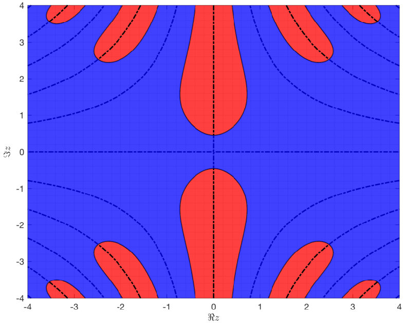
Refer to caption

Refer to caption

Figure 11. The sign charts of s⁡(z,t,γ):=1−γ​e−12​t2​z2s(z;t,\gamma):=1-\gamma\mathrm{e}^{-\frac{1}{2}t^{2}z^{2}} with γ=0.9\gamma=0.9 for t=1t=1 on the left and t=2t=2 on the right. In red values z∈ℂz\in\mathbb{C} where ℜ⁡s⁡(z,t,γ)<0\Re s(z;t,\gamma)<0 and in blue where ℜ⁡s⁡(z,t,γ)>0\Re s(z;t,\gamma)>0. Also ℑ⁡s⁡(z,t,γ)=0\Im s(z;t,\gamma)=0 along the dash-dotted black curves.

In order to proceed we now introduce the gg-function,

g⁡(z)≡g⁡(z,t,γ):=12​π​i​∫−∞∞h⁡(s,t,γ)s−z​𝑑s,z∈ℂ∖ℝg(z)\equiv g(z;t,\gamma):=\frac{1}{2\pi\mathrm{i}}\int_{-\infty}^{\infty}\frac{h(s;t,\gamma)}{s-z}\,{\mathrm{d}}s,\ \ \ z\in\mathbb{C}\setminus\mathbb{R} (5.4)

and consider the following transformation after (5.1),

𝐒⁡(z,t,γ):=𝐓⁡(z,t,γ)​eg⁡(z)​σ3,z∈ℂ∖ℝ.{\bf S}(z;t,\gamma):={\bf T}(z;t,\gamma)\mathrm{e}^{g(z)\sigma_{3}},\ \ \ z\in\mathbb{C}\setminus\mathbb{R}. (5.5)

Since h⁡(⋅,t,γ)h(\cdot;t,\gamma) is of Hoelder class on ℝ\mathbb{R} for all γ∈(0,1)\gamma\in(0,1) and t<0t<0, the classical Plemelj-Sokhotski formula applies and we arrive at the RHP below.

Riemann-Hilbert Problem 5.2.

For any t<0t<0 and γ∈(0,1)\gamma\in(0,1), the function 𝐒⁡(z)=𝐒⁡(z,t,γ)∈ℂ2×2{\bf S}(z)={\bf S}(z;t,\gamma)\in\mathbb{C}^{2\times 2} defined in (5.5) has the following properties.

  1. (1)

    𝐒⁡(z){\bf S}(z) is analytic for z∈ℂ∖ℝz\in\mathbb{C}\setminus\mathbb{R} and admits continuous boundary values on the closed upper and lower half-planes.

  2. (2)

    Along the real axis, with 𝐒±​(z)=limϵ↓0𝐒⁡(z±i​ϵ),z∈ℝ{\bf S}_{\pm}(z)=\lim_{\epsilon\downarrow 0}{\bf S}(z\pm\mathrm{i}\epsilon),z\in\mathbb{R},

    𝐒+​(z)=𝐒−​(z)​[1−i​γ​e−t2​ϕ+​(z)−i​γ​e−t2​ϕ−​(z)1−γ​e−12​t2​z2],z∈ℝ,{\bf S}_{+}(z)={\bf S}_{-}(z)\begin{bmatrix}1&-\mathrm{i}\sqrt{\gamma}\mathrm{e}^{-t^{2}\phi_{+}(z)}\\ -\mathrm{i}\sqrt{\gamma}\mathrm{e}^{-t^{2}\phi_{-}(z)}&1-\gamma\mathrm{e}^{-\frac{1}{2}t^{2}z^{2}}\end{bmatrix},\ \ \ \ z\in\mathbb{R}, (5.6)

    where

    ϕ±​(z)≡ϕ±​(z,t,γ):=θ±​(z)±1i​π​pv​∫−∞∞h⁡(s,t,γ)t2​(s−z)​𝑑s,z∈ℝ.\phi_{\pm}(z)\equiv\phi_{\pm}(z;t,\gamma):=\theta_{\pm}(z)\pm\frac{1}{\mathrm{i}\pi}\,\textnormal{pv}\int_{-\infty}^{\infty}\frac{h(s;t,\gamma)}{t^{2}(s-z)}\,{\mathrm{d}}s,\ \ \ z\in\mathbb{R}.
  3. (3)

    As z→∞,z∉ℝz\rightarrow\infty,z\notin\mathbb{R},

    𝐒⁡(z)=𝕀+𝐒1​(t,γ)​z−1+𝒪⁡(z−2),𝐒1​(t,γ)=𝐓1​(t,γ)−i​σ3t​2​π​Li32​(γ){\bf S}(z)=\mathbb{I}+{\bf S}_{1}(t,\gamma)z^{-1}+\mathcal{O}\big(z^{-2}\big),\ \ \ \ \ {\bf S}_{1}(t,\gamma)={\bf T}_{1}(t,\gamma)-\frac{\mathrm{i}\sigma_{3}}{t\sqrt{2\pi}}\textnormal{Li}_{\frac{3}{2}}(\gamma)

Our next step relies on the matrix factorization

[1−i​γ​e−t2​ϕ+​(z)−i​γ​e−t2​ϕ−​(z)1−γ​e−12​t2​z2]=[10−i​γ​e−t2​ϕ−​(z)1]​[1−i​γ​e−t2​ϕ+​(z)01],z∈ℝ,\begin{bmatrix}1&-\mathrm{i}\sqrt{\gamma}\mathrm{e}^{-t^{2}\phi_{+}(z)}\\ -\mathrm{i}\sqrt{\gamma}\mathrm{e}^{-t^{2}\phi_{-}(z)}&1-\gamma\mathrm{e}^{-\frac{1}{2}t^{2}z^{2}}\end{bmatrix}=\begin{bmatrix}1&0\\ -\mathrm{i}\sqrt{\gamma}\mathrm{e}^{-t^{2}\phi_{-}(z)}&1\end{bmatrix}\begin{bmatrix}1&-\mathrm{i}\sqrt{\gamma}\mathrm{e}^{-t^{2}\phi_{+}(z)}\\ 0&1\end{bmatrix},\ \ z\in\mathbb{R}, (5.7)

and the Lemma below.

Lemma 5.3.

The function

ϕ⁡(z)≡ϕ⁡(z,t,γ):=14​(z2−4​i​z​sgn​(ℑ⁡z))+1i​π​sgn​(ℑ⁡z)​∫−∞∞h⁡(s,t,γ)t2​(s−z)​𝑑s−1t2​h​(z,t,γ),z∈Πt​γ∖ℝ\phi(z)\equiv\phi(z;t,\gamma):=\frac{1}{4}\big(z^{2}-4\mathrm{i}z\,\textnormal{sgn}(\Im z)\big)+\frac{1}{\mathrm{i}\pi}\textnormal{sgn}(\Im z)\int_{-\infty}^{\infty}\frac{h(s;t,\gamma)}{t^{2}(s-z)}\,{\mathrm{d}}s-\frac{1}{t^{2}}h(z;t,\gamma),\ \ z\in\Pi_{t\gamma}\setminus\mathbb{R}

defined with the principal branch of the logarithm (see Proposition 5.1) is analytic in Πt​γ∖ℝ\Pi_{t\gamma}\setminus\mathbb{R} for all γ∈(0,1)\gamma\in(0,1) and t<0t<0. Moreover,

limϵ↓0ϕ⁡(z±i​ϵ)=ϕ±​(z),z∈ℝ.\lim_{\epsilon\downarrow 0}\phi(z\pm\mathrm{i}\epsilon)=\phi_{\pm}(z),\ \ \ z\in\mathbb{R}.
Proof.

Since h⁡(⋅,t,γ)h(\cdot;t,\gamma) is of Hoelder class on ℝ\mathbb{R} and analytic in Πt​γ\Pi_{t\gamma} by Proposition 5.1, the claims follow easily from the Plemelj-Sokhotski theorem. ∎

More precisely, we introduce for any γ∈(0,1)\gamma\in(0,1) and t<0t<0,

𝐌⁡(z,t,γ):=𝐒⁡(z,t,γ)​{[1i​γ​e−t2​ϕ​(z)01],z∈Ω1=Ω1​(δt​γ)[10−i​γ​e−t2​ϕ​(z)1],z∈Ω2=Ω2​(δt​γ)𝕀,elsewith​ 0<δt​γ:=min⁡{−ln⁡γ|t|,12}{\bf M}(z;t,\gamma):={\bf S}(z;t,\gamma)\begin{cases}\Bigl[\begin{smallmatrix}1&\mathrm{i}\sqrt{\gamma}\,\mathrm{e}^{-t^{2}\phi(z)}\\ 0&1\end{smallmatrix}\Bigr],&z\in\Omega_{1}=\Omega_{1}(\delta_{t\gamma})\\ \Bigl[\begin{smallmatrix}1&0\\ -\mathrm{i}\sqrt{\gamma}\,\mathrm{e}^{-t^{2}\phi(z)}&1\end{smallmatrix}\Bigr],&z\in\Omega_{2}=\Omega_{2}(\delta_{t\gamma})\\ \mathbb{I},&\textnormal{else}\end{cases}\ \ \ \textnormal{with}\ \ \ 0<\delta_{t\gamma}:=\min\left\{\frac{\sqrt{-\ln\gamma}}{|t|},\frac{1}{2}\right\} (5.8)

which leads to the RHP formulated on the red contour Σ𝐌\Sigma_{{\bf M}} in Figure 12 and with the following characteristica.

ℜ⁡z\Re zℑ⁡z\Im zℑ⁡z=δt​γ\Im z=\delta_{t\gamma}ℑ⁡z=−δt​γ\Im z=-\delta_{t\gamma}Ω1\Omega_{1}Ω2\Omega_{2}
Figure 12. The oriented jump contour Σ𝐌\Sigma_{{\bf M}} in RHP 5.4. We fix z1=−2,z2,3=−1±i​δt​γ,z3,4=1±i​δt​γz_{1}=-2,z_{2,3}=-1\pm\mathrm{i}\delta_{t\gamma},z_{3,4}=1\pm\mathrm{i}\delta_{t\gamma} and z5=2z_{5}=2 as location of the six vertices.
Riemann-Hilbert Problem 5.4.

For any γ∈(0,1)\gamma\in(0,1) and t<0t<0, the function 𝐌⁡(z)=𝐌⁡(z,t,γ)∈ℂ2×2{\bf M}(z)={\bf M}(z;t,\gamma)\in\mathbb{C}^{2\times 2} has the following properties.

  1. (1)

    𝐌⁡(z){\bf M}(z) is analytic for z∈ℂ∖Σ𝐌z\in\mathbb{C}\setminus\Sigma_{{\bf M}} and all eight straight lines are oriented from left to right, see Figure 12.

  2. (2)

    The square integrable limiting values obey

    𝐌+​(z)=𝐌−​(z)​[1−i​γ​e−t2​ϕ​(z)01],z∈Σ𝐌∩{z∈ℂ:ℑ⁡z>0};{\bf M}_{+}(z)={\bf M}_{-}(z)\begin{bmatrix}1&-\mathrm{i}\sqrt{\gamma}\mathrm{e}^{-t^{2}\phi(z)}\\ 0&1\end{bmatrix},\ \ z\in\Sigma_{{\bf M}}\cap\{z\in\mathbb{C}:\,\Im z>0\};

    and

    𝐌+​(z)=𝐌−​(z)​[10−i​γ​e−t2​ϕ​(z)1],z∈Σ𝐌∩{z∈ℂ:ℑ⁡z<0};{\bf M}_{+}(z)={\bf M}_{-}(z)\begin{bmatrix}1&0\\ -\mathrm{i}\sqrt{\gamma}\mathrm{e}^{-t^{2}\phi(z)}&1\end{bmatrix},\ \ z\in\Sigma_{{\bf M}}\cap\{z\in\mathbb{C}:\,\Im z<0\};

    as well as

    𝐌+​(z)=𝐌−​(z)​[1−i​γ​e−t2​ϕ+​(z)−i​γ​e−t2​ϕ−​(z)1−γ​e−12​t2​z2],z∈ℝ∖[−2,2].{\bf M}_{+}(z)={\bf M}_{-}(z)\begin{bmatrix}1&-\mathrm{i}\sqrt{\gamma}\mathrm{e}^{-t^{2}\phi_{+}(z)}\\ -\mathrm{i}\sqrt{\gamma}\mathrm{e}^{-t^{2}\phi_{-}(z)}&1-\gamma\mathrm{e}^{-\frac{1}{2}t^{2}z^{2}}\end{bmatrix},\ \ z\in\mathbb{R}\setminus[-2,2].

    By construction, see Lemma 5.3 and equation (5.7), there is no jump along (−2,2)⊂ℝ(-2,2)\subset\mathbb{R}.

  3. (3)

    For large |z||z| the leading order asymptotic behavior of RHP 5.2 is unchanged,

    𝐌⁡(z)=𝕀+𝐒1​(t,γ)​z−1+𝒪⁡(z−2),z→∞.{\bf M}(z)=\mathbb{I}+{\bf S}_{1}(t,\gamma)z^{-1}+\mathcal{O}\big(z^{-2}\big),\ \ \ z\rightarrow\infty.

We now proceed with the necessary small norm estimates for the jump matrix 𝐆𝐌​(z,t,γ){\bf G}_{{\bf M}}(z;t,\gamma) in condition (2) of RHP 5.4. And since we are about to investigate the limit γ↑1\gamma\uparrow 1 in the upcoming sections we shall already now indicate the γ\gamma-dependency in all error estimates.

Proposition 5.5.

There exists positive universal constants t0,cjt_{0},c_{j} such that for any γ∈(0,1)\gamma\in(0,1),

‖𝐆𝐌​(⋅,t,γ)−𝕀‖L∞​(Σ𝐌,|d​z|)≤c1​γ14​e−t2​δt​γ1−γ,‖𝐆𝐌​(⋅,t,γ)−𝕀‖L2​(Σ𝐌,|d​z|)≤c2​γ14​e−t2​δt​γ1−γ​|t|−12,\|{\bf G}_{{\bf M}}(\cdot;t,\gamma)-\mathbb{I}\|_{L^{\infty}(\Sigma_{{\bf M}},|{\mathrm{d}}z|)}\leq c_{1}\frac{\gamma^{\frac{1}{4}}\mathrm{e}^{-t^{2}\delta_{t\gamma}}}{1-\gamma},\ \ \ \ \ \ \ \|{\bf G}_{{\bf M}}(\cdot;t,\gamma)-\mathbb{I}\|_{L^{2}(\Sigma_{{\bf M}},|{\mathrm{d}}z|)}\leq c_{2}\frac{\gamma^{\frac{1}{4}}\mathrm{e}^{-t^{2}\delta_{t\gamma}}}{1-\gamma}\,|t|^{-\frac{1}{2}}, (5.9)

hold true for all (−t)≥t0(-t)\geq t_{0}.

Proof.

For z∈ℝ∖[−2,2]z\in\mathbb{R}\setminus[-2,2] we clearly have ‖𝐆𝐌​(⋅,t,γ)−𝕀‖=𝒪⁡(e−t2)\|{\bf G}_{{\bf M}}(\cdot;t,\gamma)-\mathbb{I}\|=\mathcal{O}(\mathrm{e}^{-t^{2}}) in L2∩L∞L^{2}\cap L^{\infty} and thus no contribution to the leading order in (5.9). Next, for z∈ℂ∖ℝz\in\mathbb{C}\setminus\mathbb{R},

e−t2​ϕ​(z)=e−t2​θ±​(z)1−γ​e−12​t2​z2exp[±iπ∫−∞∞h⁡(s,t,γ)s−zds],\mathrm{e}^{-t^{2}\phi(z)}=\frac{\mathrm{e}^{-t^{2}\theta_{\pm}(z)}}{1-\gamma\mathrm{e}^{-\frac{1}{2}t^{2}z^{2}}}\,\exp\left[\pm\frac{\mathrm{i}}{\pi}\int_{-\infty}^{\infty}\frac{h(s;t,\gamma)}{s-z}\,{\mathrm{d}}s\right],

so we have to estimate three factors. With the parametrizations z=z⁡(λ)=λ±i​δt​γ,λ∈[−1,1]z=z(\lambda)=\lambda\pm\mathrm{i}\delta_{t\gamma},\lambda\in[-1,1] we find

|e−t2​θ±​(z⁡(λ))|≤e−t2​δt​γ−14​t2​λ2​γ−14,|1−γ​e−12​t2​z2​(λ)|=[1−2​γ​e−12​t2​(λ2−δt​γ)​cos⁡(t2​λ​δt​γ)+γ2​e−t2​(λ2−δt​γ2)]12\left|\mathrm{e}^{-t^{2}\theta_{\pm}(z(\lambda))}\right|\leq\mathrm{e}^{-t^{2}\delta_{t\gamma}-\frac{1}{4}t^{2}\lambda^{2}}\gamma^{-\frac{1}{4}},\ \ \left|1-\gamma\mathrm{e}^{-\frac{1}{2}t^{2}z^{2}(\lambda)}\right|=\left[1-2\gamma\mathrm{e}^{-\frac{1}{2}t^{2}(\lambda^{2}-\delta_{t\gamma})}\cos(t^{2}\lambda\delta_{t\gamma})+\gamma^{2}\mathrm{e}^{-t^{2}(\lambda^{2}-\delta_{t\gamma}^{2})}\right]^{\frac{1}{2}}

and

|exp[±iπ∫−∞∞h⁡(s,t,γ)s−z⁡(λ)ds]|=exp[−δt​γπ∫−∞∞h⁡(s,t,γ)(s−λ)2+δt​γ2ds].\left|\exp\left[\pm\frac{\mathrm{i}}{\pi}\int_{-\infty}^{\infty}\frac{h(s;t,\gamma)}{s-z(\lambda)}\,{\mathrm{d}}s\right]\right|=\exp\left[-\frac{\delta_{t\gamma}}{\pi}\int_{-\infty}^{\infty}\frac{h(s;t,\gamma)}{(s-\lambda)^{2}+\delta_{t\gamma}^{2}}\,{\mathrm{d}}s\right]. (5.10)

Hence,

supλ∈[−1,1]|e−t2​θ±​(z⁡(λ))1−γ​e−12​t2​z2​(λ)|≤γ−14​e−t2​δt​γ1−γ,\sup_{\lambda\in[-1,1]}\left|\frac{\mathrm{e}^{-t^{2}\theta_{\pm}(z(\lambda))}}{1-\gamma\mathrm{e}^{-\frac{1}{2}t^{2}z^{2}(\lambda)}}\right|\leq\frac{\gamma^{-\frac{1}{4}}\mathrm{e}^{-t^{2}\delta_{t\gamma}}}{1-\sqrt{\gamma}},

and since the integrand in (5.10) is non-negative we have therefore established the above L∞L^{\infty} estimate. For the L2L^{2} estimate we use Laplace’s method for the factor exp⁡[−t2​θ±​(z)]\exp[-t^{2}\theta_{\pm}(z)] and the same reasonings that were used in the second and third while deriving the previous L∞L^{\infty} estimate. For the four slanted straight lines consider, say, z=z⁡(λ)=λ−2±i​λ​δt​γz=z(\lambda)=\lambda-2\pm\mathrm{i}\lambda\delta_{t\gamma} with λ∈[0,1]\lambda\in[0,1]. Then,

|e−t2​θ±​(z⁡(λ))|=e−14​t2​(λ2​(1−δt​γ2)−4​λ​(1−δt​γ)+4),\left|\mathrm{e}^{-t^{2}\theta_{\pm}(z(\lambda))}\right|=\mathrm{e}^{-\frac{1}{4}t^{2}(\lambda^{2}(1-\delta_{t\gamma}^{2})-4\lambda(1-\delta_{t\gamma})+4)},

as well as

|1−γ​e−12​t2​z2​(λ)|=[1−2​γ​e−12​t2​((λ−2)2−λ2​δt​γ2)​cos⁡(t2​λ​(λ−2)​δt​γ)+γ2​e−t2​((λ−2)2−λ2​δt​γ2)]12,\left|1-\gamma\mathrm{e}^{-\frac{1}{2}t^{2}z^{2}(\lambda)}\right|=\left[1-2\gamma\mathrm{e}^{-\frac{1}{2}t^{2}((\lambda-2)^{2}-\lambda^{2}\delta_{t\gamma}^{2})}\cos\big(t^{2}\lambda(\lambda-2)\delta_{t\gamma}\big)+\gamma^{2}\mathrm{e}^{-t^{2}((\lambda-2)^{2}-\lambda^{2}\delta_{t\gamma}^{2})}\right]^{\frac{1}{2}},

and

|exp[±iπ∫−∞∞h⁡(s,t,γ)s−z⁡(λ)ds]|=exp[−λ​δt​γπ∫−∞∞h⁡(s,t,γ)(s−λ+2)2+λ2​δt​γ2ds].\left|\exp\left[\pm\frac{\mathrm{i}}{\pi}\int_{-\infty}^{\infty}\frac{h(s;t,\gamma)}{s-z(\lambda)}\,{\mathrm{d}}s\right]\right|=\exp\left[-\frac{\lambda\delta_{t\gamma}}{\pi}\int_{-\infty}^{\infty}\frac{h(s;t,\gamma)}{(s-\lambda+2)^{2}+\lambda^{2}\delta_{t\gamma}^{2}}\,{\mathrm{d}}s\right]. (5.11)

Thus

supλ∈[0,1]|e−t2​θ±​(z⁡(λ))1−γ​e−12​t2​z2​(λ)|≤e−14​t2​(1−δt​γ2)1−γ​e−12​t2​(1−δt​γ2),\sup_{\lambda\in[0,1]}\left|\frac{\mathrm{e}^{-t^{2}\theta_{\pm}(z(\lambda))}}{1-\gamma\mathrm{e}^{-\frac{1}{2}t^{2}z^{2}(\lambda)}}\right|\leq\frac{\mathrm{e}^{-\frac{1}{4}t^{2}(1-\delta_{t\gamma}^{2})}}{1-\gamma\mathrm{e}^{-\frac{1}{2}t^{2}(1-\delta_{t\gamma}^{2})}},

which is of sub-leading order for γ∈(0,1)\gamma\in(0,1) when compared to (5.9), see (5.7). By non-negativity of the integrand in (5.11) we have therefore completed our proof. ∎

Since we are dealing with a (t,γ)(t,\gamma)-dependent contour in RHP 5.4 (the hexagon in Figure 12 is collapsing to the real axis as t→−∞t\rightarrow-\infty or γ↑1\gamma\uparrow 1) the general framework of [13] is not directly applicable to Proposition 5.5. Still, using somewhat similar ideas as in [7], the results of Appendix A below guarantee unique solvability of RHP 5.4 in L2​(Σ𝐌,|d​z|)L^{2}(\Sigma_{{\bf M}},|{\mathrm{d}}z|) for all (−t)≥t0(-t)\geq t_{0} and either any fixed γ∈(0,1)\gamma\in(0,1) or γ↑1\gamma\uparrow 1 at a certain controlled rate.

Theorem 5.6.

For any fixed 0<ϵ<20<\epsilon<2, RHP 5.4 is uniquely solvable in L2​(Σ𝐌,|d​z|)L^{2}(\Sigma_{{\bf M}},|{\mathrm{d}}z|) for (−t)(-t) sufficiently large and all 0<γ≤1−|t|−ϵ0<\gamma\leq 1-|t|^{-\epsilon}. Moreover,

𝐒1​(t,γ)=limz→∞z⁡(𝐌⁡(z,t,γ)−𝕀)=𝒪⁡(|t|−1+ϵ​e−|t|1−ϵ2),∀(−t)≥t0, 0<γ≤1−|t|−ϵ.{\bf S}_{1}(t,\gamma)=\lim_{z\rightarrow\infty}z\big({\bf M}(z;t,\gamma)-\mathbb{I}\big)=\mathcal{O}\left(|t|^{-1+\epsilon}\mathrm{e}^{-|t|^{1-\frac{\epsilon}{2}}}\right),\ \ \ \forall\ (-t)\geq t_{0},\ \ 0<\gamma\leq 1-|t|^{-\epsilon}. (5.12)

5.2. Left tail asymptotics

In order to complete the derivation of (1.16), we first recall (3.14), transformations (3.18), (5.1), (5.5), (5.7),

∂∂tlndet(1−γTχt↾L2​(ℝ))=12​πLi32(γ)+itS122(t,γ).\frac{\partial}{\partial t}\ln\det(1-\gamma T\chi_{t}\upharpoonright_{L^{2}(\mathbb{R})})=\frac{1}{\sqrt{2\pi}}\textnormal{Li}_{\frac{3}{2}}(\gamma)+\mathrm{i}tS_{1}^{22}(t,\gamma).

Thus, with Theorem 5.6 and an indefinite tt-integration,

Proposition 5.7.

For any fixed 0<ϵ<20<\epsilon<2, there exist positive constants t0=t0​(ϵ)t_{0}=t_{0}(\epsilon) and c=c⁡(ϵ)c=c(\epsilon) such that

lndet(1−γTχt↾L2​(ℝ))=t2​πLi32(γ)+D1(γ)+r1(t,γ),\ln\det(1-\gamma T\chi_{t}\upharpoonright_{L^{2}(\mathbb{R})})=\frac{t}{\sqrt{2\pi}}\textnormal{Li}_{\frac{3}{2}}(\gamma)+D_{1}(\gamma)+r_{1}(t,\gamma),

for all (−t)≥t0(-t)\geq t_{0} and 0<γ≤1−|t|−ϵ0<\gamma\leq 1-|t|^{-\epsilon}. The term D1​(γ)D_{1}(\gamma) is tt-independent and we record the error estimate

|r1​(t,γ)|≤c⁡(ϵ)​|t|32​ϵ​e−|t|1−ϵ2∀(−t)≥t0and​ 0<γ≤1−|t|−ϵ.\big|r_{1}(t,\gamma)\big|\leq c(\epsilon)|t|^{\frac{3}{2}\epsilon}\mathrm{e}^{-|t|^{1-\frac{\epsilon}{2}}}\ \ \ \forall\,(-t)\geq t_{0}\ \ \textnormal{and}\ \ 0<\gamma\leq 1-|t|^{-\epsilon}.

Next we use the estimate (based again on the transformations (3.18), (5.1), (5.5), (5.7) and Theorem 5.6)

∫t∞Y112​(x,γ)​𝑑x=I⁡(γ)−∫−∞tY112​(x,γ)​𝑑x=I⁡(γ)+∫−∞tx​S112​(x,γ)​𝑑x=I⁡(γ)+𝒪⁡(|t|32​ϵ​e−|t|1−ϵ2),\int_{t}^{\infty}Y_{1}^{12}(x,\gamma)\,{\mathrm{d}}x=I(\gamma)-\int_{-\infty}^{t}Y_{1}^{12}(x,\gamma)\,{\mathrm{d}}x=I(\gamma)+\int_{-\infty}^{t}xS_{1}^{12}(x,\gamma)\,{\mathrm{d}}x=I(\gamma)+\mathcal{O}\left(|t|^{\frac{3}{2}\epsilon}\mathrm{e}^{-|t|^{1-\frac{\epsilon}{2}}}\right),

where I⁡(γ)I(\gamma) denotes the total integral of Y112​(x,γ)Y_{1}^{12}(x,\gamma) over x∈ℝx\in\mathbb{R}. From this, with (4.19) and Γt​γ=1−uγ​(t)\Gamma_{t\gamma}=1-u^{\gamma}(t) we obtain in turn

Proposition 5.8.

For any fixed 0<ϵ<20<\epsilon<2, there exist positive constants t0=t0​(ϵ)t_{0}=t_{0}(\epsilon) and c=c⁡(ϵ)c=c(\epsilon) such that

ln⁡Γt​γ=D2​(γ)+r2​(t,γ)\ln\Gamma_{t\gamma}=D_{2}(\gamma)+r_{2}(t,\gamma)

for all (−t)≥t0(-t)\geq t_{0} and 0<γ≤1−|t|−ϵ0<\gamma\leq 1-|t|^{-\epsilon}. The term D2​(γ)D_{2}(\gamma) is tt-independent and we record the error estimate

|r2​(t,γ)|≤c⁡(ϵ)​|t|32​ϵ​e−|t|1−ϵ2∀(−t)≥t0and​ 0<γ≤1−|t|−ϵ.\big|r_{2}(t,\gamma)\big|\leq c(\epsilon)|t|^{\frac{3}{2}\epsilon}\mathrm{e}^{-|t|^{1-\frac{\epsilon}{2}}}\ \ \ \forall\,(-t)\geq t_{0}\ \ \textnormal{and}\ \ 0<\gamma\leq 1-|t|^{-\epsilon}.

Once we combine Propositions 5.7 and 5.8, Corollary 1.9, expansion (1.16) follows easily.

6. Proof of Theorem 1.11

The following lines are near copies of the argument given in [15] in the derivation of the analogue of (1.17) for the GOE. First, by (1.1) and (1.3),

(F(t))2=det(1−Tχt↾L2​(ℝ))Γt=det(1−(T+U⊗V)↾L2​(t,∞)),\big(F(t)\big)^{2}=\det(1-T\chi_{t}\upharpoonright_{L^{2}(\mathbb{R})})\Gamma_{t}=\det\big(1-(T+U\otimes V)\upharpoonright_{L^{2}(t,\infty)}\big), (6.1)

where U⊗VU\otimes V denotes the finite rank integral operator on L2​(t,∞)L^{2}(t,\infty) with kernel

(U⊗V)​(x,y)=g⁡(x)​G​(y),g⁡(x)=1π​e−x2,G⁡(x)=∫−∞xg⁡(y)​𝑑y,(U\otimes V)(x,y)=g(x)G(y),\ \ \ \ \ g(x)=\frac{1}{\sqrt{\pi}}\,\mathrm{e}^{-x^{2}},\ \ \ G(x)=\int_{-\infty}^{x}g(y)\,{\mathrm{d}}y,

i.e. UU is the operator which multiplies by g⁡(x)g(x) and VV the integral operator with kernel G⁡(y)G(y). Indeed, (6.1) follows by noting that for any operator AA we have A⁡(U⊗V)=(A​U⊗V)A(U\otimes V)=(AU\otimes V), applying the factorization

det(1−(T+U⊗V)↾L2​(t,∞))=det(1−T↾L2​(t,∞))det(1−(1−T)−1(U⊗V)↾L2​(t,∞)),\det\big(1-(T+U\otimes V)\upharpoonright_{L^{2}(t,\infty)}\big)=\det(1-T\upharpoonright_{L^{2}(t,\infty)})\det\big(1-(1-T)^{-1}(U\otimes V)\upharpoonright_{L^{2}(t,\infty)}\big), (6.2)

and using the eigenvector/value equation (see [18, Chapter 9.79.7] for a similar argument in the GOE)

((1−T)−1(U⊗V)↾L2​(t,∞)F)(x)=[∫t∞G(y)((1−T↾L2​(t,∞))−1g)(y)dy]F(x),\big((1-T)^{-1}(U\otimes V)\upharpoonright_{L^{2}(t,\infty)}F\big)(x)=\left[\int_{t}^{\infty}G(y)\big((1-T\upharpoonright_{L^{2}(t,\infty)})^{-1}g\big)(y)\,{\mathrm{d}}y\right]F(x), (6.3)

where

F(x)=((1−T↾L2​(t,∞))−1g)(x).F(x)=\big((1-T\upharpoonright_{L^{2}(t,\infty)})^{-1}g\big)(x).

Precisely, (6.3) computes the finite rank operator determinant in (6.2) as

det(1−(1−T)−1(U⊗V)↾L2​(t,∞))=1−∫t∞G(y)((1−T↾L2​(t,∞))−1g)(y)dy=Γt,\det\big(1-(1-T)^{-1}(U\otimes V)\upharpoonright_{L^{2}(t,\infty)}\big)=1-\int_{t}^{\infty}G(y)\big((1-T\upharpoonright_{L^{2}(t,\infty)})^{-1}g\big)(y)\,{\mathrm{d}}y=\Gamma_{t},

and (6.1) follows from (6.2) since det(1−T↾L2​(t,∞))=det(1−Tχt↾L2​(ℝ))\det(1-T\upharpoonright_{L^{2}(t,\infty)})=\det(1-T\chi_{t}\upharpoonright_{L^{2}(\mathbb{R})}). Secondly, it will be more convenient to move the tt-dependency in the right-hand side of (6.1) into the integral operators,

(F(t))2=det(1−(Tt+Ut⊗Vt)↾L2​(0,∞)),t∈ℝ,\big(F(t)\big)^{2}=\det\big(1-(T_{t}+U_{t}\otimes V_{t})\upharpoonright_{L^{2}(0,\infty)}\big),\ \ \ t\in\mathbb{R}, (6.4)

where Tt:L2​(0,∞)→L2​(0,∞)T_{t}:L^{2}(0,\infty)\rightarrow L^{2}(0,\infty) has kernel Tt​(x,y)=T⁡(x+t,y+t)T_{t}(x,y)=T(x+t,y+t), compare (1.2), UtU_{t} is multiplcation by g⁡(x+t)g(x+t) and VtV_{t} has kernel G⁡(y+t)G(y+t). Thirdly, we note that Tt=St​StT_{t}=S_{t}S_{t} where St:L2​(0,∞)→L2​(0,∞)S_{t}:L^{2}(0,\infty)\rightarrow L^{2}(0,\infty) has kernel

St​(x,y)=1π​e−(x+y+t)2,x,y>0.S_{t}(x,y)=\frac{1}{\sqrt{\pi}}\mathrm{e}^{-(x+y+t)^{2}},\ \ \ x,y>0.
Lemma 6.1.

For every t∈ℝt\in\mathbb{R}, the operator StS_{t} satisfies ‖St‖≤1\|S_{t}\|\leq 1 and 1∓St1\mp S_{t} are invertible on L2​(0,∞)L^{2}(0,\infty).

Proof.

Since StS_{t} is self-adjoint we have for any f∈L2​(0,∞)f\in L^{2}(0,\infty),

‖St​f‖L2​(0,∞)2=⟨St​f,St​f⟩L2​(0,∞)=⟨f,St2​f⟩L2​(0,∞)=⟨f,Tt​f⟩L2​(0,∞)≤(2.3)⟨f,f⟩L2​(0,∞),\|S_{t}f\|^{2}_{L^{2}(0,\infty)}=\langle S_{t}f,S_{t}f\rangle_{L^{2}(0,\infty)}=\langle f,S_{t}^{2}f\rangle_{L^{2}(0,\infty)}=\langle f,T_{t}f\rangle_{L^{2}(0,\infty)}\stackrel{{\scriptstyle\eqref{l:3}}}{{\leq}}\langle f,f\rangle_{L^{2}(0,\infty)},

and therefore

‖St‖=sup‖f‖L2​(0,∞)=1‖St​f‖L2​(0,∞)≤1.\|S_{t}\|=\sup_{\|f\|_{L^{2}(0,\infty)}=1}\|S_{t}f\|_{L^{2}(0,\infty)}\leq 1.

Also, (1−St)​(1+St)=(1+St)​(1−St)=1−Tt(1-S_{t})(1+S_{t})=(1+S_{t})(1-S_{t})=1-T_{t} on L2​(0,∞)L^{2}(0,\infty) and since 1−Tt1-T_{t} is invertible by Lemma 2.1, so are 1∓St1\mp S_{t}. ∎

The last Lemma allows us to transform the right-hand side in (6.4) through the following factorization,

det\displaystyle\det (1−(St2+Ut⊗Vt)↾L2​(0,∞))=det(1−St↾L2​(0,∞))det(1+St−(1−St)−1(Ut⊗Vt)↾L2​(0,∞))\displaystyle\big(1-(S_{t}^{2}+U_{t}\otimes V_{t})\upharpoonright_{L^{2}(0,\infty)}\big)=\det(1-S_{t}\upharpoonright_{L^{2}(0,\infty)})\det\big(1+S_{t}-(1-S_{t})^{-1}(U_{t}\otimes V_{t})\upharpoonright_{L^{2}(0,\infty)}\big)
=\displaystyle= det(1−St↾L2​(0,∞))det(1+St−(Ut⊗W)↾L2​(0,∞)),\displaystyle\,\det(1-S_{t}\upharpoonright_{L^{2}(0,\infty)})\det\big(1+S_{t}-(U_{t}\otimes W)\upharpoonright_{L^{2}(0,\infty)}\big), (6.5)

where WW multiplies by the characteristic function χ0​(x)\chi_{0}(x).33 3 Evidently, χ0\chi_{0} and the later on used δ0\delta_{0} are not in L2​(0,∞)L^{2}(0,\infty). Still, using regularity and decay properties of the involved integral kernels all subsequent Fredholm determinant and inner product manipulations are justifiable, we refer the interested reader to [31, Section VIII]. To get to (6.5) we have used that for any operator AA we have A⁡(U⊗V)=(U⊗A∗​V)A(U\otimes V)=(U\otimes A^{\ast}V) in terms of the real adjoint A∗A^{\ast} and that

G(x+t)=1−∫0∞St(x,y)dy=((1−St↾L2​(0,∞))χ0)(x),χ0(x)={1,x≥00,x<0.G(x+t)=1-\int_{0}^{\infty}S_{t}(x,y)\,{\mathrm{d}}y=\big((1-S_{t}\upharpoonright_{L^{2}(0,\infty)})\chi_{0}\big)(x),\ \ \ \ \ \chi_{0}(x)=\begin{cases}1,&x\geq 0\\ 0,&x<0\end{cases}.

Continuing with (6.5), another factorization yields

det(1+StCLOSE\displaystyle\det\big(1+S_{t} −(Ut⊗W)↾L2​(0,∞))=det(1+St↾L2​(0,∞))det(1−(1+St)−1(Ut⊗W)↾L2​(0,∞))\displaystyle-(U_{t}\otimes W)\upharpoonright_{L^{2}(0,\infty)}\big)=\det(1+S_{t}\upharpoonright_{L^{2}(0,\infty)})\det\big(1-(1+S_{t})^{-1}(U_{t}\otimes W)\upharpoonright_{L^{2}(0,\infty)}\big)
=det(1+St↾L2​(0,∞)){1−∫0∞χ0(y)((1+St↾L2​(0,∞))−1g)(y+t)dy}\displaystyle=\det(1+S_{t}\upharpoonright_{L^{2}(0,\infty)})\left\{1-\int_{0}^{\infty}\chi_{0}(y)\big((1+S_{t}\upharpoonright_{L^{2}(0,\infty)})^{-1}g\big)(y+t)\,{\mathrm{d}}y\right\} (6.6)

where we have used a variation of the eigenvector/value trick (6.3) in the last equality. Since

g⁡(x+t)=∫0∞St​(x,y)​δ0​(y)​𝑑y=(St​δ0)​(x);∫0∞f⁡(x)​δ0​(x)​𝑑x:=f⁡(0),g(x+t)=\int_{0}^{\infty}S_{t}(x,y)\delta_{0}(y)\,{\mathrm{d}}y=\big(S_{t}\delta_{0}\big)(x);\ \ \ \ \ \ \int_{0}^{\infty}f(x)\delta_{0}(x)\,{\mathrm{d}}x:=f(0),

for any test function ff we can simplify the second factor in (6.6) further,

1−∫0∞χ0​(y)​((1+CLOSECLOSE\displaystyle 1-\int_{0}^{\infty}\chi_{0}(y)\big((1+ St↾L2​(0,∞))−1g)(y+t)dy=∫0∞χ0(y)((1−(1+St)−1St↾L2​(0,∞))δ0)(y)dy\displaystyle S_{t}\upharpoonright_{L^{2}(0,\infty)})^{-1}g\big)(y+t)\,{\mathrm{d}}y=\int_{0}^{\infty}\chi_{0}(y)\Big(\big(1-(1+S_{t})^{-1}S_{t}\upharpoonright_{L^{2}(0,\infty)}\big)\delta_{0}\Big)(y)\,{\mathrm{d}}y
=∫0∞χ0(y)((1+St↾L2​(0,∞))−1δ0)(y)dy=⟨χ0,(1+St↾L2​(0,∞))−1δ0⟩L2​(0,∞)\displaystyle\,=\int_{0}^{\infty}\chi_{0}(y)\big((1+S_{t}\upharpoonright_{L^{2}(0,\infty)})^{-1}\delta_{0}\big)(y)\,{\mathrm{d}}y=\big\langle\chi_{0},(1+S_{t}\upharpoonright_{L^{2}(0,\infty)})^{-1}\delta_{0}\big\rangle_{L^{2}(0,\infty)} (6.7)

The proof of Theorem 1.11 would thus be completed through (6.5), (6.6), (6.7) and the identity det(1−St↾L2​(0,∞))=det(1−Sχt↾L2​(ℝ))\det(1-S_{t}\upharpoonright_{L^{2}(0,\infty)})=\det(1-S\chi_{t}\upharpoonright_{L^{2}(\mathbb{R})}) if we manage to proof the following

det(1−St↾L2​(0,∞))=det(1+St↾L2​(0,∞))⟨χ0,(1+St↾L2​(0,∞))−1δ0⟩L2​(0,∞),t∈ℝ;\det(1-S_{t}\upharpoonright_{L^{2}(0,\infty)})=\det(1+S_{t}\upharpoonright_{L^{2}(0,\infty)})\big\langle\chi_{0},(1+S_{t}\upharpoonright_{L^{2}(0,\infty)})^{-1}\delta_{0}\big\rangle_{L^{2}(0,\infty)},\ \ t\in\mathbb{R}; (6.8)

or equivalently (taking logarithmic derivatives, then observing the unity normalization of all three factors in (6.8) as t→+∞t\rightarrow+\infty, using Lemma 6.1 and self-adjointness),

trL2​(0,∞)((1−St2)−1d​Std​t)=−12dd​tln⟨δ0,(1+St↾L2​(0,∞))−1χ0⟩L2​(0,∞).\mathop{\mathrm{tr}}\limits_{L^{2}(0,\infty)}\left((1-S_{t}^{2})^{-1}\frac{{\mathrm{d}}S_{t}}{{\mathrm{d}}t}\right)=-\frac{1}{2}\frac{{\mathrm{d}}}{{\mathrm{d}}t}\ln\big\langle\delta_{0},(1+S_{t}\upharpoonright_{L^{2}(0,\infty)})^{-1}\chi_{0}\big\rangle_{L^{2}(0,\infty)}. (6.9)

But integrating by parts in the left-hand side of (6.9) with dd​t​St​(x,y)=dd​x​St​(x,y)=dd​y​St​(x,y)\frac{{\mathrm{d}}}{{\mathrm{d}}t}S_{t}(x,y)=\frac{{\mathrm{d}}}{{\mathrm{d}}x}S_{t}(x,y)=\frac{{\mathrm{d}}}{{\mathrm{d}}y}S_{t}(x,y) shows that (cf. [15, Lemma 22]),

trL2​(0,∞)((1−St2)−1d​Std​t)=−12⟨δ0,((1−St2)−1St↾L2​(0,∞))δ0⟩L2​(0,∞),\mathop{\mathrm{tr}}\limits_{L^{2}(0,\infty)}\left((1-S_{t}^{2})^{-1}\frac{{\mathrm{d}}S_{t}}{{\mathrm{d}}t}\right)=-\frac{1}{2}\big\langle\delta_{0},((1-S_{t}^{2})^{-1}S_{t}\upharpoonright_{L^{2}(0,\infty)})\delta_{0}\big\rangle_{L^{2}(0,\infty)},

so we need to establish the equality

⟨δ0,((1−St2)−1St↾L2​(0,∞))δ0⟩L2​(0,∞)=dd​tln⟨δ0,(1+St↾L2​(0,∞))−1χ0⟩L2​(0,∞).\big\langle\delta_{0},((1-S_{t}^{2})^{-1}S_{t}\upharpoonright_{L^{2}(0,\infty)})\delta_{0}\big\rangle_{L^{2}(0,\infty)}=\frac{{\mathrm{d}}}{{\mathrm{d}}t}\ln\big\langle\delta_{0},(1+S_{t}\upharpoonright_{L^{2}(0,\infty)})^{-1}\chi_{0}\big\rangle_{L^{2}(0,\infty)}. (6.10)
Lemma 6.2.

[15, Lemma 33] Let Δ0\Delta_{0} denote multiplication by δ0​(x)\delta_{0}(x), and DD (=dd​x)(=\frac{{\mathrm{d}}}{{\mathrm{d}}x}) differentiation. Then

dd​t​(1+St)−1=(1−St2)−1​St​D+(1−St2)−1​St​Δ0​(1+St)−1.\frac{{\mathrm{d}}}{{\mathrm{d}}t}(1+S_{t})^{-1}=(1-S_{t}^{2})^{-1}S_{t}D+(1-S_{t}^{2})^{-1}S_{t}\Delta_{0}(1+S_{t})^{-1}. (6.11)
Proof.

Integrating by parts, we easily find that D​St=−St​Δ0−St​DDS_{t}=-S_{t}\Delta_{0}-S_{t}D, or equivalently

−(1−St)​D​St=St​D​(1+St)+St​Δ0.-(1-S_{t})DS_{t}=S_{t}D(1+S_{t})+S_{t}\Delta_{0}.

Multiplying this last identity by (1−St2)−1(1-S_{t}^{2})^{-1} from the left and (1+St)−1(1+S_{t})^{-1} from the right (recall Lemma 6.1),

−(1+St)−1​D​St​(1+St)−1=(1−St2)−1​St​D+(1−St2)−1​St​Δ0​(1+St)−1,-(1+S_{t})^{-1}DS_{t}(1+S_{t})^{-1}=(1-S_{t}^{2})^{-1}S_{t}D+(1-S_{t}^{2})^{-1}S_{t}\Delta_{0}(1+S_{t})^{-1},

and the last left-hand side equals precisely dd​t​(1+St)−1\frac{{\mathrm{d}}}{{\mathrm{d}}t}(1+S_{t})^{-1} because of the simple fact that

dd​t​(1+St)−1=−(1+St)−1​d​Std​t​(1+St)−1,\frac{{\mathrm{d}}}{{\mathrm{d}}t}(1+S_{t})^{-1}=-(1+S_{t})^{-1}\frac{{\mathrm{d}}S_{t}}{{\mathrm{d}}t}(1+S_{t})^{-1},

and dd​t​St​(x,y)=dd​x​St​(x,y)\frac{{\mathrm{d}}}{{\mathrm{d}}t}S_{t}(x,y)=\frac{{\mathrm{d}}}{{\mathrm{d}}x}S_{t}(x,y). Identity (6.11) is thus proven. ∎

We now use (6.11) in the right-hand side of (6.10) (suppressing at times the Hilbert space references for compact notation),

dd​tln⟨δ0,(1+\displaystyle\frac{{\mathrm{d}}}{{\mathrm{d}}t}\ln\big\langle\delta_{0},(1+ St↾L2​(0,∞))−1χ0⟩L2​(0,∞)=⟨δ0,dd​t(1+St↾L2​(0,∞))−1χ0⟩L2​(0,∞)⟨δ0,(1+St↾L2​(0,∞))−1χ0⟩L2​(0,∞)\displaystyle S_{t}\upharpoonright_{L^{2}(0,\infty)})^{-1}\chi_{0}\big\rangle_{L^{2}(0,\infty)}=\frac{\langle\delta_{0},\frac{{\mathrm{d}}}{{\mathrm{d}}t}(1+S_{t}\upharpoonright_{L^{2}(0,\infty)})^{-1}\chi_{0}\rangle_{L^{2}(0,\infty)}}{\langle\delta_{0},(1+S_{t}\upharpoonright_{L^{2}(0,\infty)})^{-1}\chi_{0}\rangle_{L^{2}(0,\infty)}}
=D​χ0=0\displaystyle\stackrel{{\scriptstyle D\chi_{0}=0}}{{=}} ⟨δ0,(1−St2)−1​St​Δ0​(1+St)−1​χ0⟩⟨δ0,(1+St)−1​χ0⟩=⟨δ0,(1−St2)−1​St​δ0⟩​⟨δ0,(1+St)−1​χ0⟩⟨δ0,(1+St)−1​χ0⟩\displaystyle\,\,\frac{\langle\delta_{0},(1-S_{t}^{2})^{-1}S_{t}\Delta_{0}(1+S_{t})^{-1}\chi_{0}\rangle}{\langle\delta_{0},(1+S_{t})^{-1}\chi_{0}\rangle}=\frac{\langle\delta_{0},(1-S_{t}^{2})^{-1}S_{t}\delta_{0}\rangle\langle\delta_{0},(1+S_{t})^{-1}\chi_{0}\rangle}{\langle\delta_{0},(1+S_{t})^{-1}\chi_{0}\rangle}
=\displaystyle= ⟨δ0,((1−St2)−1St↾L2​(0,∞))δ0⟩L2​(0,∞),\displaystyle\,\,\langle\delta_{0},((1-S_{t}^{2})^{-1}S_{t}\upharpoonright_{L^{2}(0,\infty)})\delta_{0}\rangle_{L^{2}(0,\infty)},

which is (6.10). In turn the proof of Theorem 1.11 is thus completed.

Appendix A Small norm estimates for collapsing contours

The jump contour Σ𝐌\Sigma_{{\bf M}} of RHP 5.4 collapses for large (−t)(-t) to the real axis and we shall invoke ideas from [7] in the solution of the underlying singular integral equation ([7] does not apply verbatim to RHP 5.4 as we are not dealing with contracting disk contours, for those the scaling invariance of z−1​d​zz^{-1}{\mathrm{d}}z is central).

Write Σ𝐌=⋃j=18Σj\Sigma_{{\bf M}}=\bigcup_{j=1}^{8}\Sigma_{j} as union of the eight straight lines shown in Figure 13 below and suppose ρ∈L2​(Σ𝐌,|d​z|)\rho\in L^{2}(\Sigma_{{\bf M}},|{\mathrm{d}}z|) is a 2×22\times 2 matrix-valued function which is Lipschitz on Σj\Sigma_{j} and that satisfies

ρ⁡(z)=𝕀+12​π​i​∫Σ𝐌ρ⁡(λ)​(𝐆𝐌​(λ)−𝕀)​d​λλ−z−,z∈Σj,\rho(z)=\mathbb{I}+\frac{1}{2\pi\mathrm{i}}\int_{\Sigma_{{\bf M}}}\rho(\lambda)\big({\bf G}_{{\bf M}}(\lambda)-\mathbb{I}\big)\frac{{\mathrm{d}}\lambda}{\lambda-z_{-}},\ \ \ z\in\Sigma_{j}, (A.1)

where z−z_{-} denotes the limiting value of the integral from the right side. The explicit form of the jump matrix 𝐆𝐌​(z)=𝐆𝐌​(z,t,γ){\bf G}_{\bf M}(z)={\bf G}_{\bf M}(z;t,\gamma) is stated in RHP 5.4, condition (2).

Lemma A.1.

On each Σj\Sigma_{j} the function

𝐌⁡(z):=𝕀+12​π​i​∫Σ𝐌ρ⁡(λ)​(𝐆𝐌​(λ)−𝕀)​d​λλ−z,z∈ℂ∖Σ𝐌{\bf M}(z):=\mathbb{I}+\frac{1}{2\pi\mathrm{i}}\int_{\Sigma_{{\bf M}}}\rho(\lambda)\big({\bf G}_{{\bf M}}(\lambda)-\mathbb{I}\big)\frac{{\mathrm{d}}\lambda}{\lambda-z},\ \ \ z\in\mathbb{C}\setminus\Sigma_{{\bf M}}

satisfies

𝐌+​(z)=𝐌−​(z)​𝐆𝐌​(z),z∈Σj.{\bf M}_{+}(z)={\bf M}_{-}(z){\bf G}_{{\bf M}}(z),\ \ \ z\in\Sigma_{j}.
Proof.

Since 𝐌−​(z)=ρ​(z){\bf M}_{-}(z)=\rho(z) for z∈Σjz\in\Sigma_{j} the jump behavior of the Cauchy transform implies

𝐌+​(z)−𝐌−​(z)=ρ⁡(z)​(𝐆𝐌​(z)−𝕀)=𝐌−​(z)​(𝐆𝐌​(z)−𝕀),z∈Σj.{\bf M}_{+}(z)-{\bf M}_{-}(z)=\rho(z)\big({\bf G}_{{\bf M}}(z)-\mathbb{I}\big)={\bf M}_{-}(z)\big({\bf G}_{{\bf M}}(z)-\mathbb{I}\big),\ \ z\in\Sigma_{j}.

∎

ℜ⁡z\Re zℑ⁡z\Im zΣ1\Sigma_{1}Σ2\Sigma_{2}Σ3\Sigma_{3}Σ6\Sigma_{6}Σ7\Sigma_{7}Σ4\Sigma_{4}Σ5\Sigma_{5}Σ8\Sigma_{8}
Figure 13. The oriented jump contour Σ𝐌=⋃j=18Σj\Sigma_{{\bf M}}=\bigcup_{j=1}^{8}\Sigma_{j} in RHP 5.4.

We shall now solve (A.1) in L2​(Σ𝐌,|d​z|)L^{2}(\Sigma_{{\bf M}},|{\mathrm{d}}z|) by the Neumann series

ρ⁡(z)=𝕀+∑k=1∞ρk​(z);ρk​(z)\displaystyle\rho(z)=\mathbb{I}+\sum_{k=1}^{\infty}\rho_{k}(z);\ \ \ \ \ \ \ \ \rho_{k}(z) =\displaystyle= 12​π​i​∫Σ𝐌ρk−1​(λ)​(𝐆𝐌​(λ)−𝕀)​d​λλ−z−,z∈Σ𝐌,k∈ℤ≥1\displaystyle\frac{1}{2\pi\mathrm{i}}\int_{\Sigma_{{\bf M}}}\rho_{k-1}(\lambda)\big({\bf G}_{{\bf M}}(\lambda)-\mathbb{I}\big)\frac{{\mathrm{d}}\lambda}{\lambda-z_{-}},\ \ z\in\Sigma_{{\bf M}},\ k\in\mathbb{Z}_{\geq 1}
ρ0​(z)\displaystyle\rho_{0}(z) =\displaystyle= 𝕀,\displaystyle\mathbb{I},

and thus need to estimate ρk​(z)\rho_{k}(z). Recall that L2​(Σ𝐌,|d​z|)L^{2}(\Sigma_{{\bf M}},|{\mathrm{d}}z|) is the space of (matrix-valued) measurable functions such that

‖f‖L2​(Σ𝐌,|d​z|)={∫Σ𝐌‖f⁡(z)‖2​|𝑑z|}12<∞.\|f\|_{L^{2}(\Sigma_{{\bf M}},|{\mathrm{d}}z|)}=\left\{\int_{\Sigma_{{\bf M}}}\|f(z)\|^{2}|{\mathrm{d}}z|\right\}^{\frac{1}{2}}<\infty.

Let CΣj±C_{\Sigma_{j}}^{\pm} denote the Cauchy operators on L2​(Σ𝐌,|d​z|)L^{2}(\Sigma_{{\bf M}},|{\mathrm{d}}z|),

(CΣj±​ρ)​(z)=limϵ↓0∫Σjρ⁡(s)s−(z±i​ϵ)​d​s2​π​i,z∈Σj,(C_{\Sigma_{j}}^{\pm}\rho)(z)=\lim_{\epsilon\downarrow 0}\int_{\Sigma_{j}}\frac{\rho(s)}{s-(z\pm\mathrm{i}\epsilon)}\frac{{\mathrm{d}}s}{2\pi\mathrm{i}},\ \ z\in\Sigma_{j},

which obey (cf. [28, Chapter II] or [2, Section 5.55.5])

CΣj+−CΣj−=id,CΣj++CΣj−=iHΣj,a.e. onΣj;(HΣjρ)(z)=1πpv∫Σjρ(λ)d​sz−s.C_{\Sigma_{j}}^{+}-C_{\Sigma_{j}}^{-}=\textnormal{id},\ \ \ \ \ C_{\Sigma_{j}}^{+}+C_{\Sigma_{j}}^{-}=\mathrm{i}H_{\Sigma_{j}},\ \ \textnormal{a.e. on}\ \Sigma_{j};\ \ \ \ (H_{\Sigma_{j}}\rho)(z)=\frac{1}{\pi}\,\textnormal{pv}\int_{\Sigma_{j}}\rho(\lambda)\frac{{\mathrm{d}}s}{z-s}. (A.2)
Proposition A.2 ([11], Theoreme I).

If an oriented contour Γ⊂ℂ\Gamma\subset\mathbb{C}, given by the parametric equations

Γ={z∈ℂ:ℜz=t∈ℝ,ℑz=ϕ(t)}\Gamma=\{z\in\mathbb{C}:\ \Re z=t\in\mathbb{R},\ \Im z=\phi(t)\}

satisfies a uniform Lipschitz condition, i.e. there exists M≥0M\geq 0 such that

|ϕ⁡(x)−ϕ⁡(y)|≤M​|x−y|,\big|\phi(x)-\phi(y)\big|\leq M|x-y|,

then there exists a universal C0>0C_{0}>0 such that

‖HΓ​f‖L2​(Γ,|d​z|)≤C0​(1+M)10​‖f‖L2​(Γ,|d​z|).\|H_{\Gamma}f\|_{L^{2}(\Gamma,|{\mathrm{d}}z|)}\leq C_{0}(1+M)^{10}\|f\|_{L^{2}(\Gamma,|{\mathrm{d}}z|)}. (A.3)

Observe that our eight pieces Σj\Sigma_{j} fit into the context of Proposition A.2 with a (t,γ)(t,\gamma)-independent constant MM, thus we are now prepared to the derive our central estimate.

Theorem A.3.

For any γ∈(0,1)\gamma\in(0,1) and t<0t<0, let Σ𝐌=⋃j=18Σj\Sigma_{{\bf M}}=\bigcup_{j=1}^{8}\Sigma_{j} denote the (t,γ)(t,\gamma)-dependent contour of RHP 5.4. Then there exists a universal constant K>0K>0 such that

‖HΣ𝐌​f‖L2​(Σ𝐌,|d​z|)≤K​ln⁡(δt​γ−1)​‖f‖L2​(Σ𝐌,|d​z|).\|H_{\Sigma_{{\bf M}}}f\|_{L^{2}(\Sigma_{{\bf M}},|{\mathrm{d}}z|)}\leq K\ln(\delta_{t\gamma}^{-1})\,\|f\|_{L^{2}(\Sigma_{{\bf M}},|{\mathrm{d}}z|)}. (A.4)
Proof.

We show that for some K^>0\widehat{K}>0,

|⟨HΣ𝐌​(χΣj​f),χΣk​g⟩L2​(Σ𝐌,|d​z|)|≤K^​ln⁡(δt​γ−1)​‖f‖L2​(Σ𝐌,|d​z|)​‖g‖L2​(Σ𝐌,|d​z|), 1≤j,k≤8.\big|\langle H_{\Sigma_{{\bf M}}}(\chi_{\Sigma_{j}}f),\chi_{\Sigma_{k}}g\rangle_{L^{2}(\Sigma_{{\bf M}},|{\mathrm{d}}z|)}\big|\leq\widehat{K}\ln(\delta_{t\gamma}^{-1})\,\|f\|_{L^{2}(\Sigma_{{\bf M}},|{\mathrm{d}}z|)}\|g\|_{L^{2}(\Sigma_{{\bf M}},|{\mathrm{d}}z|)},\ \ \ \ 1\leq j,k\leq 8.

Indeed, for j=kj=k this follows at once from (A.3) and for j≠kj\neq k we use the following estimates (derived from the Cauchy-Schwarz inequality while using polar coordinates and standard manipulations)

∫−11∫−11|f⁡(x+i​δγ​t)​g​(y−i​δt​γ)|(x−y)2+4​δt​γ2​𝑑x​𝑑y≤\displaystyle\int_{-1}^{1}\int_{-1}^{1}\frac{|f(x+\mathrm{i}\delta_{\gamma t})g(y-\mathrm{i}\delta_{t\gamma})|}{\sqrt{(x-y)^{2}+4\delta_{t\gamma}^{2}}}\,{\mathrm{d}}x\,{\mathrm{d}}y\,\leq C1​ln⁡(δt​γ−1)​‖f‖L2​(Σ4,|d​z|)​‖g‖L2​(Σ5,|d​z|);\displaystyle\,\,C_{1}\ln(\delta_{t\gamma}^{-1})\,\|f\|_{L^{2}(\Sigma_{4},|{\mathrm{d}}z|)}\|g\|_{L^{2}(\Sigma_{5},|{\mathrm{d}}z|)};
∫0∞∫0∞|f⁡(x)​g​(y)|(x−y)2+δt​γ2​x2​𝑑x​𝑑y≤\displaystyle\int_{0}^{\infty}\int_{0}^{\infty}\frac{|f(x)g(y)|}{\sqrt{(x-y)^{2}+\delta_{t\gamma}^{2}x^{2}}}\,{\mathrm{d}}x\,{\mathrm{d}}y\,\leq C2​ln⁡(δt​γ−1)​‖f‖L2​(0,∞)​‖g‖L2​(0,∞),Cj>0;\displaystyle\,\,C_{2}\ln(\delta_{t\gamma}^{-1})\|f\|_{L^{2}(0,\infty)}\|g\|_{L^{2}(0,\infty)},\ \ \ \ C_{j}>0;
∫0∞∫0∞|f⁡(x)​g​(y)|x+y​𝑑x​𝑑y≤\displaystyle\int_{0}^{\infty}\int_{0}^{\infty}\frac{|f(x)g(y)|}{x+y}\,{\mathrm{d}}x\,{\mathrm{d}}y\,\leq C3​‖f‖L2​(0,∞)​‖g‖L2​(0,∞).\displaystyle\,\,C_{3}\|f\|_{L^{2}(0,\infty)}\|g\|_{L^{2}(0,\infty)}.

∎

From estimate (A.4) we derive the operator norm estimate

∥HΣ𝐌∥L2​(Σ𝐌,|d​z|)≤Kln(δt​γ−1),K>0universal\|H_{\Sigma_{{\bf M}}}\|_{L^{2}(\Sigma_{{\bf M}},|{\mathrm{d}}z|)}\leq K\ln(\delta_{t\gamma}^{-1}),\ \ \ \ K>0\ \ \textnormal{universal}

and then in turn, with (A.2),

‖CΣ𝐌±‖L2​(Σ𝐌,|d​z|)≤12​(K+1)​ln⁡(δt​γ−1),∀(−t)≥t0,γ∈(0,1).\|C_{\Sigma_{{\bf M}}}^{\pm}\|_{L^{2}(\Sigma_{{\bf M}},|{\mathrm{d}}z|)}\leq\frac{1}{2}(K+1)\ln(\delta_{t\gamma}^{-1}),\ \ \forall\,(-t)\geq t_{0},\ \ \ \gamma\in(0,1). (A.5)

Returning now to the iterates {ρk​(z)}k=0∞\{\rho_{k}(z)\}_{k=0}^{\infty} introduced above, we have

ρk​(z)=(CΣ𝐌−​[ρk−1​(𝐆𝐌−𝕀)])​(z),z∈Σ𝐌.\rho_{k}(z)=\Big(C^{-}_{\Sigma_{{\bf M}}}\big[\rho_{k-1}({\bf G}_{{\bf M}}-\mathbb{I})\big]\Big)(z),\ \ \ z\in\Sigma_{{\bf M}}.

But

‖ρk−1​(𝐆𝐌−𝕀)‖L2​(Σ𝐌,|d​z|)≤‖𝐆𝐌​(⋅,t,γ)−𝕀‖L∞​(Σ𝐌)⋅‖ρk−1‖L2​(Σ𝐌,|d​z|),\|\rho_{k-1}({\bf G}_{{\bf M}}-\mathbb{I})\|_{L^{2}(\Sigma_{{\bf M}},|{\mathrm{d}}z|)}\leq\|{\bf G}_{{\bf M}}(\cdot;t,\gamma)-\mathbb{I}\|_{L^{\infty}(\Sigma_{{\bf M}})}\cdot\|\rho_{k-1}\|_{L^{2}(\Sigma_{{\bf M}},|{\mathrm{d}}z|)},

and for all (−t)≥t0,γ∈(0,1)(-t)\geq t_{0},\gamma\in(0,1),

‖ρ1‖L2​(Σ𝐌,|d​z|)=‖CΣ𝐌−​(𝐆𝐌−𝕀)‖L2​(Σ𝐌,|d​z|)≤12​(K+1)​ln⁡(δt​γ−1)⋅‖𝐆𝐌​(⋅,t,γ)−𝕀‖L2​(Σ𝐌,|d​z|),\|\rho_{1}\|_{L^{2}(\Sigma_{{\bf M}},|{\mathrm{d}}z|)}=\|C^{-}_{\Sigma_{{\bf M}}}({\bf G}_{{\bf M}}-\mathbb{I})\|_{L^{2}(\Sigma_{{\bf M}},|{\mathrm{d}}z|)}\leq\frac{1}{2}(K+1)\ln(\delta_{t\gamma}^{-1})\cdot\|{\bf G}_{{\bf M}}(\cdot;t,\gamma)-\mathbb{I}\|_{L^{2}(\Sigma_{{\bf M}},|{\mathrm{d}}z|)},

so that with Proposition 5.5,

Proposition A.4.

There exist positive universal constants t0,ct_{0},c such that for any γ∈(0,1)\gamma\in(0,1),

‖ρk‖L2​(Σ𝐌γ,|d​z|)≤(c​ln⁡(δt​γ−1)​e−t2​δt​γ1−γ)k​|t|−12,∀(−t)≥t0,k∈ℤ≥1.\|\rho_{k}\|_{L^{2}(\Sigma_{{\bf M}_{\gamma}},|{\mathrm{d}}z|)}\leq\left(c\ln(\delta_{t\gamma}^{-1})\frac{\mathrm{e}^{-t^{2}\delta_{t\gamma}}}{1-\gamma}\right)^{k}|t|^{-\frac{1}{2}},\ \ \ \forall\,(-t)\geq t_{0},\ \ k\in\mathbb{Z}_{\geq 1}.

Thus, given any 0<ϵ<20<\epsilon<2, Proposition A.4 implies convergence of the Neumann series 𝕀+∑k=1∞ρk​(z)\mathbb{I}+\sum_{k=1}^{\infty}\rho_{k}(z) in L2​(Σ𝐌,|d​z|)L^{2}(\Sigma_{{\bf M}},|{\mathrm{d}}z|) for sufficiently large (−t)≥t0(-t)\geq t_{0} and any γ∈(0,1)\gamma\in(0,1) such that 0<γ≤1−|t|−ϵ0<\gamma\leq 1-|t|^{-\epsilon}. At this point, using ρ⁡(z)\rho(z), we define

𝐌⁡(z):=𝕀+12​π​i​∫Σ𝐌ρ⁡(λ)​(𝐆𝐌​(λ)−𝕀)​d​λλ−z,z∈ℂ∖Σ𝐌{\bf M}(z):=\mathbb{I}+\frac{1}{2\pi\mathrm{i}}\int_{\Sigma_{{\bf M}}}\rho(\lambda)\big({\bf G}_{{\bf M}}(\lambda)-\mathbb{I}\big)\frac{{\mathrm{d}}\lambda}{\lambda-z},\ \ \ z\in\mathbb{C}\setminus\Sigma_{{\bf M}} (A.6)

which coincides with the function 𝐌⁡(z){\bf M}(z) defined by (5.7) (compare Lemma A.1 and the argument in [7, (A.37)-(A.39)] near a triple point, a point on Σ𝐌\Sigma_{{\bf M}} where three arcs meet). Thus, compare RHP 5.4,

𝐒1​(t,γ)=limz→∞z⁡(𝐌⁡(z)−𝕀)=i2​π​∫Σ𝐌ρ⁡(λ)​(𝐆𝐌​(λ)−𝕀)​𝑑λ=∑k=0∞𝐒1​k​(t,γ),{\bf S}_{1}(t,\gamma)=\lim_{z\rightarrow\infty}z\big({\bf M}(z)-\mathbb{I}\big)=\frac{\mathrm{i}}{2\pi}\int_{\Sigma_{{\bf M}}}\rho(\lambda)\big({\bf G}_{{\bf M}}(\lambda)-\mathbb{I}\big)\,{\mathrm{d}}\lambda=\sum_{k=0}^{\infty}{\bf S}_{1k}(t,\gamma),

where

𝐒1​k​(t,γ)=i2​π​∫Σ𝐌ρk​(λ)​(𝐆𝐌​(λ)−𝕀)​𝑑λ.{\bf S}_{1k}(t,\gamma)=\frac{\mathrm{i}}{2\pi}\int_{\Sigma_{{\bf M}}}\rho_{k}(\lambda)\big({\bf G}_{{\bf M}}(\lambda)-\mathbb{I}\big)\,{\mathrm{d}}\lambda.

Since for (−t)≥t0(-t)\geq t_{0} and γ∈(0,1)\gamma\in(0,1), with Cj>0C_{j}>0,

k≥1:\displaystyle k\geq 1: ‖𝐒1​k​(t,γ)‖≤C1​‖ρk‖L2​(Σ𝐌,|d​z|)​‖𝐆𝐌​(⋅,t,γ)−𝕀‖L2​(Σ𝐌,|d​z|)≤C1​(c​ln⁡(δt​γ−1)​e−t2​δt​γ1−γ)k​e−t2​δt​γ1−γ​|t|−1,\displaystyle\,\,\,\,\,\,\|{\bf S}_{1k}(t,\gamma)\|\leq C_{1}\|\rho_{k}\|_{L^{2}(\Sigma_{{\bf M}},|{\mathrm{d}}z|)}\|{\bf G}_{{\bf M}}(\cdot;t,\gamma)-\mathbb{I}\|_{L^{2}(\Sigma_{{\bf M}},|{\mathrm{d}}z|)}\leq C_{1}\left(c\ln(\delta_{t\gamma}^{-1})\frac{\mathrm{e}^{-t^{2}\delta_{t\gamma}}}{1-\gamma}\right)^{k}\frac{\mathrm{e}^{-t^{2}\delta_{t\gamma}}}{1-\gamma}|t|^{-1},
k=0:\displaystyle k=0: ‖𝐒1​k​(t,γ)‖≤C2​‖𝐆𝐌​(⋅,t,γ)−𝕀‖L1​(Σ𝐌,|d​z|)≤C2​e−t2​δt​γ1−γ​|t|−1,\displaystyle\,\,\,\,\,\,\|{\bf S}_{1k}(t,\gamma)\|\leq C_{2}\|{\bf G}_{{\bf M}}(\cdot;t,\gamma)-\mathbb{I}\|_{L^{1}(\Sigma_{{\bf M}},|{\mathrm{d}}z|)}\leq C_{2}\frac{\mathrm{e}^{-t^{2}\delta_{t\gamma}}}{1-\gamma}|t|^{-1},

we can now sum all inequalities from k=0k=0 to k=+∞k=+\infty: for any fixed ϵ∈(0,2)\epsilon\in(0,2),

𝐒1​(t,γ)=𝒪⁡(|t|−1+ϵ​e−|t|1−ϵ2),∀(−t)≥t0, 0<γ≤1−|t|−ϵ.{\bf S}_{1}(t,\gamma)=\mathcal{O}\left(|t|^{-1+\epsilon}\mathrm{e}^{-|t|^{1-\frac{\epsilon}{2}}}\right),\ \ \ \forall\ (-t)\geq t_{0},\ \ 0<\gamma\leq 1-|t|^{-\epsilon}.

This completes the proof of Theorem 5.6.

Appendix B Permuting resolvent and integration

Let ϕ\phi and ψ\psi be two functions on ℝ\mathbb{R} that decay exponentially fast at +∞+\infty. Introduce

K⁡(x,y):=∫0∞ϕ⁡(x+s)​ψ​(y+s)​𝑑s,x,y∈ℝ,K(x,y):=\int_{0}^{\infty}\phi(x+s)\psi(y+s)\,{\mathrm{d}}s,\ \ \ \ x,y\in\mathbb{R},

and the corresponding integral operator KK on L2​(ℝ)L^{2}(\mathbb{R}) with kernel K⁡(x,y)K(x,y). For any function ff, we shall denote by fy​(x):=f⁡(x+y)f_{y}(x):=f(x+y) the horizontal translation of ff by −y-y. Then,

Proposition B.1.

For any x,y,t∈ℝx,y,t\in\mathbb{R} and k∈ℤ≥1k\in\mathbb{Z}_{\geq 1}, we have

((Kχt↾L2​(ℝ))kϕy)(x)=((Kχt↾L2​(ℝ))kϕx−t)y(t).\big((K\chi_{t}\upharpoonright_{L^{2}(\mathbb{R})})^{k}\phi_{y}\big)(x)=\big((K\chi_{t}\upharpoonright_{L^{2}(\mathbb{R})})^{k}\phi_{x-t}\big)_{y}(t). (B.1)
Proof.

We prove (B.1) inductively using

K⁡(x,y)=∫t∞ϕ⁡(x+u−t)​ψ​(y+u−t)​𝑑u.K(x,y)=\int_{t}^{\infty}\phi(x+u-t)\psi(y+u-t)\,{\mathrm{d}}u.

Indeed, for k=1k=1, we have

(Kχt↾L2​(ℝ)ϕy)(x)=∫t∞K(x,s)ϕ(s+y)ds=∫s∞∫s∞ϕ(x+u−t)ψ(s+u−t)ϕ(s+y)duds,\big(K\chi_{t}\upharpoonright_{L^{2}(\mathbb{R})}\phi_{y}\big)(x)=\int_{t}^{\infty}K(x,s)\phi(s+y)\,{\mathrm{d}}s=\int_{s}^{\infty}\int_{s}^{\infty}\phi(x+u-t)\psi(s+u-t)\phi(s+y)\,{\mathrm{d}}u\,{\mathrm{d}}s,

so that by Fubini’s theorem,

(Kχt↾L2​(ℝ)ϕy)(x)=∫t∞K(y+t,u)ϕ(u+x−t)du=(Kχt↾L2​(ℝ)ϕx−t)y(t).\big(K\chi_{t}\upharpoonright_{L^{2}(\mathbb{R})}\phi_{y}\big)(x)=\int_{t}^{\infty}K(y+t,u)\phi(u+x-t)\,{\mathrm{d}}u=\big(K\chi_{t}\upharpoonright_{L^{2}(\mathbb{R})}\phi_{x-t}\big)_{y}(t).

For general kk, assuming that (B.1) is true for k−1k-1,

((Kχt↾L2​(ℝ))kϕy)(x)=∫t∞K(x,s)((Kχt↾L2​(ℝ))k−1ϕy)(s)ds\displaystyle\hskip 28.45274pt\big((K\chi_{t}\upharpoonright_{L^{2}(\mathbb{R})})^{k}\phi_{y}\big)(x)=\int_{t}^{\infty}K(x,s)\big((K\chi_{t}\upharpoonright_{L^{2}(\mathbb{R})})^{k-1}\phi_{y}\big)(s)\,{\mathrm{d}}s
=\displaystyle= ∫t∞K(x,s)((Kχt↾L2​(ℝ))k−1ϕs−t)y(t)ds=∫t∞∫t∞K(x,s)(Kχt↾L2​(ℝ))k−1(t+y,u)ϕ(u+s−t)duds,\displaystyle\,\int_{t}^{\infty}\!K(x,s)\big((K\chi_{t}\upharpoonright_{L^{2}(\mathbb{R})})^{k-1}\phi_{s-t}\big)_{y}(t)\,{\mathrm{d}}s=\int_{t}^{\infty}\!\!\int_{t}^{\infty}\!\!K(x,s)\big(K\chi_{t}\upharpoonright_{L^{2}(\mathbb{R})}\big)^{k-1}(t+y,u)\phi(u+s-t)\,{\mathrm{d}}u\,{\mathrm{d}}s,

and thus again by Fubini’s theorem

((Kχt↾L2​(ℝ))kϕy)(x)=∫t∞(Kχt↾L2​(ℝ))k−1(t+y,u)(Kχt↾L2​(ℝ)ϕu−t)(x)du.\big((K\chi_{t}\upharpoonright_{L^{2}(\mathbb{R})})^{k}\phi_{y}\big)(x)=\int_{t}^{\infty}\big(K\chi_{t}\upharpoonright_{L^{2}(\mathbb{R})}\big)^{k-1}(t+y,u)\big(K\chi_{t}\upharpoonright_{L^{2}(\mathbb{R})}\phi_{u-t}\big)(x)\,{\mathrm{d}}u.

Now apply the base case k=1k=1 result and derive

((Kχt↾L2​(ℝ))kϕy)(x)=\displaystyle\big((K\chi_{t}\upharpoonright_{L^{2}(\mathbb{R})})^{k}\phi_{y}\big)(x)= ∫t∞(Kχt↾L2​(ℝ))k−1(t+y,u)(Kχt↾L2​(ℝ)ϕx−t)(u)du\displaystyle\,\int_{t}^{\infty}\big(K\chi_{t}\upharpoonright_{L^{2}(\mathbb{R})}\big)^{k-1}(t+y,u)\big(K\chi_{t}\upharpoonright_{L^{2}(\mathbb{R})}\phi_{x-t}\big)(u)\,{\mathrm{d}}u
=\displaystyle= ((Kχt↾L2​(ℝ))kϕx−t)(t+y)=((Kχt↾L2​(ℝ))kϕx−t)y(t),\displaystyle\,\big((K\chi_{t}\upharpoonright_{L^{2}(\mathbb{R})})^{k}\phi_{x-t}\big)(t+y)=\big((K\chi_{t}\upharpoonright_{L^{2}(\mathbb{R})})^{k}\phi_{x-t}\big)_{y}(t),

which completes the proof. ∎

The above Proposition B.1 leads to the following useful Corollary

Corollary B.2.

Let

Φ⁡(x):=∫Iϕy​(x)​𝑑y,\Phi(x):=\int_{I}\phi_{y}(x)\,{\mathrm{d}}y,

where II is a subset of ℝ\mathbb{R}. Then, for any x,t∈ℝx,t\in\mathbb{R} and k∈ℤ≥1k\in\mathbb{Z}_{\geq 1},

((Kχt↾L2​(ℝ))kΦ)(x)=∫I((Kχt↾L2​(ℝ))kϕx−t)y(t)dy.\big((K\chi_{t}\upharpoonright_{L^{2}(\mathbb{R})})^{k}\Phi\big)(x)=\int_{I}\big((K\chi_{t}\upharpoonright_{L^{2}(\mathbb{R})})^{k}\phi_{x-t}\big)_{y}(t)\,{\mathrm{d}}y. (B.2)
Proof.

We have by linearity and (B.1),

((Kχt↾L2​(ℝ))kΦ)(x)=\displaystyle\big((K\chi_{t}\upharpoonright_{L^{2}(\mathbb{R})})^{k}\Phi\big)(x)= (Kχt↾L2​(ℝ))k[∫Iϕy(⋅)dy](x)=∫I((Kχt↾L2​(ℝ))kϕy)(x)dy\displaystyle\,(K\chi_{t}\upharpoonright_{L^{2}(\mathbb{R})})^{k}\left[\int_{I}\phi_{y}(\cdot)\,{\mathrm{d}}y\right](x)=\int_{I}\big((K\chi_{t}\upharpoonright_{L^{2}(\mathbb{R})})^{k}\phi_{y}\big)(x)\,{\mathrm{d}}y
=(B.1)∫I((Kχt↾L2​(ℝ))kϕx−t)y(t)dy.\displaystyle\,\stackrel{{\scriptstyle\eqref{J:1}}}{{=}}\int_{I}\big((K\chi_{t}\upharpoonright_{L^{2}(\mathbb{R})})^{k}\phi_{x-t}\big)_{y}(t)\,{\mathrm{d}}y.

∎

References

  • [1] M. Ablowitz, P. Clarkson, Solitons, nonlinear evolution equations and inverse scattering. Cambridge University Press, Cambridge, UK, 1991
  • [2] J. Baik, P. Deift, T. Suidan, Combinatorics and random matrix theory. American Mathematical Soc. 172 (2016)
  • [3] R. Beals, R. Coifman, Scattering and inverse scattering for first order systems, Comm. Pure Appl. Math. 37 (1984), no. 1, 39-90
  • [4] R. Beals, P. Deift, C. Tomei, Direct and inverse scattering on the line. American Mathematical Soc. 28 (2015)
  • [5] M. Bertola, M. Cafasso, The transition between the gap probabilities from the Pearcey to the Airy process - a Riemann-Hilbert approach, International Mathematics Research Notices (2011), doi:10.1093/imrn/rnr066.
  • [6] M. Bertola, M. Cafasso, Riemann-Hilbert approach to multi-time processes: The Airy and the Pearcey cases, Physica D 241, 2237-2245 (2012)
  • [7] P. Bleher, A. Kuijlaars, Large n limit of Gaussian random matrices with external source, part III, Commun. Math. Phys. 270, 481-517 (2007)
  • [8] F. Bornemann, On the numerical evaluation of Fredholm determinants, Mathematics of computation, Volume 79, Number 270, April 2010, Pages 871-915
  • [9] A. Borodin, P. Deift, Fredholm determinants, Jimbo-Miwa-Ueno τ\tau-functions, and representation theory, Comm. Pure Appl. Math. 55 (2002), no. 9, 1160-1230
  • [10] T. Bothner, R. Buckingham, Large deformations of the Tracy-Widom distribution I. Non-oscillatory asymptotics, Commun. Math. Phys. 359, 223-263 (2018)
  • [11] R. Coifman, A. McIntosh, Y. Meyer, L’intégrale de Cauchy définit un opérateur borné sur L2L^{2} pour les courbes Lipschitziennes, Ann. Math. 116, 361-387 (1982)
  • [12] P. Deift, Orthogonal polynomials and random matrices: a Riemann-Hilbert approach. Courant Lecture Notes in Mathematics, 3. New York University, Courant Institute of Mathematical Sciences, New York; American Mathematical Society, Providence, RI, 1999.
  • [13] P. Deift, X. Zhou, A steepest descent method for oscillatory Riemann-Hilbert problems. Asymptotics for the MKdV equation, Ann. of Math. (2) 137 (1993), no. 2, 295-368.
  • [14] A. Edelman, Eigenvalues and condition numbers of random matrices, SIAM J. Matrix Anal. Appl. 9 543-560 (1988)
  • [15] P. Ferrari, H. Spohn, A determinantal formula for the GOE Tracy-Widom distribution, J. Phys. A: Math. Gen. 38 (2005) L557-L561
  • [16] A. Fokas, U. Mugan, X. Zhou, On the solvability of Painlevé I, III and V, Inverse Problems 8 (1992), 757-785
  • [17] A. Fokas, X. Zhou, On the solvability of Painlevé II and IV, Commun. Math. Phys. 144 (1992), 601-622.
  • [18] P. Forrester, Log-Gases and Random Matrices, Princeton University Press, Princeton, NJ, 2010.
  • [19] P. Forrester, Diffusion processes and the asymptotic bulk gap probability for the real Ginibre ensemble, J. Phys. A: Math. Theor. 48 324001 (2015)
  • [20] P. Forrester, T. Nagao, Eigenvalue statistics of the real Ginibre ensemble, Physical Review Letters, Vol. 99, (2007)
  • [21] J. Ginibre, Statistical ensembles of complex, quaternion, and real matrices, Journal of Mathematical Physics, 6, 440 (1965)
  • [22] I. Gohberg, S. Goldberg, N. Krupnik, Traces and determinants of linear operators, Operator Theory Advances and Applications, Vol. 116, Birkhäuser Verlag, Basel, (2000)
  • [23] A. Its, A. Izergin, V. Korepin, N. Slavnov, Differential equations for quantum correlation functions. Int. J. Mod. Phys. B 4, 1003-1037 (1990)
  • [24] NIST, Digital Library of Mathematical Functions, http://dlmf.nist.gov
  • [25] M. Poplavskyi, R. Tribe, O. Zaboronski, On the distribution of the largest real eigenvalue for the real Ginibre ensemble, The Annals of Applied Probability, 2017, Vol. 27, No. 3, 1395-1413
  • [26] B. Rider, C. Sinclair, Extremal laws for the real Ginibre ensemble, The Annals of Applied Probability, 2014, Vol. 24, No. 4, 1621-1651
  • [27] B. Simon, Basic complex analysis. A comprehensive course in analysis, Part 2A. American Mathematical Society, Providence, RI, 2015.
  • [28] E. Stein, Singular integrals and differentiability properties of functions, Princeton Mathematical Series, 30. Princeton University Press, Princeton, N.J., 1970
  • [29] T. Tao, V. Vu, Random matrices: universality of ESDs and the circular law, The Annals of Probability, Vol. 38, No. 5, 2023-2065 (2010)
  • [30] C. Tracy, H. Widom, Fredholm determinants, differential equations and matrix models, Commun. Math. Phys. 163, 33-72 (1994)
  • [31] C. Tracy, H. Widom, On orthogonal and symplectic matrix ensembles, Commun. Math. Phys. 177, 727-754 (1996)
  • [32] V. Zakharov , A. Shabat, Exact theory of two-dimensional self-focusing and one-dimensional self-modulation of waves in nonlinear media, Soviet Physics JETP, 34(1):62-69, 1972.
  • [33] X. Zhou, The Riemann-Hilbert problem and inverse scattering, SIAM J. Math. Anal. 20 (1989), 966-986