Approximate stabilizer rank and improved weak simulation of Clifford-dominated circuits for qudits
Abstract
Bravyi and Gosset recently gave classical simulation algorithms for quantum circuits dominated by Clifford operations. These algorithms scale exponentially with the number of -gates in the circuit, but polynomially in the number of qubits and Clifford operations. Here we extend their algorithm to qudits of odd prime dimension. We generalize their approximate stabilizer rank method for weak simulation to qudits and obtain the scaling of the approximate stabilizer rank with the number of single-qudit magic states. We also relate the canonical form of qudit stabilizer states to Gauss sum evaluations and give an algorithm for calculating the inner product of two -qudit stabilizer states.
I Introduction
With the prospect of noisy intermediate scale quantum (NISQ) computers with qubits appearing in the next decade [4, 30], determining the minimal classical cost of simulation of quantum computers has received much recent attention [8, 35, 18, 5, 29].
The Gottesman-Knill theorem shows that Clifford circuits are efficiently classically simulatable [1]. Adding any non-Clifford gate creates a universal gate set 11 1 An elegant recent presentation of this result in group-theoretic terms is given in [nebe2001invariants] and is briefly summarized in [11]. One such choice for a non-Clifford gate is the gate: [6]. Bravyi and Gosset gave a classical algorithm for simulation of quantum circuits that scales exponentially with the number of -gates in the circuit but polynomially with the number of qubits and Clifford gates [8]. This algorithm was further developed in [7].
What is supplied by the addition of -gates to a Clifford circuit? The fault tolerant implementation of Clifford+ circuits substitutes magic states for each gate [9, 40]. Colloquially, gates add “magic” to a Clifford circuit. Magic is supplied by contextuality, a longstanding source of puzzles and paradoxes in the foundations of quantum mechanics [23].
The relationship of magic to contextuality also provides a connection to quasiprobability representations of quantum mechanics [36, 13, 13]. Specifically, positivity of a quasiprobability representation is equivalent to the absence of contextuality, and such positive states, operations and measurements admit efficient classical simulation in some cases [38, 28]. Classical statistical theories with an imposed uncertainty principle can reproduce these positive quasiprobabilistic theories for Gaussian states and qudits with [37, 3].
Pashayan et al. gave an algorithm allowing a positive quasiprobability description to include some negativity [34]. Comparing the algorithms of Bravyi and Gosset and Pashayan should shed more light on the relationship between magic, contextuality and negativity [8, 34]. However quasiprobability representations for qubits are distinct from their -dimensional cousins [24, 25, 26]. The desire to understand the relationship between magic, contextuality and negativity therefore motivates extension of the algorithm of Bravyi and Gosset to qudits with dimension greater than two. In the present paper we extend the algorithm of Bravyi and Gosset to qudits of odd prime dimension.
The structure of the paper is as follows. In Sections II and III, we briefly introduce the necessary background. In Section IV we give the nonorthogonal decomposition of the magic state, and in Section V we give results on approximate stabilizer rank and weak simulation algorithm for qudits. We close the paper by briefly comparing our algorithm to that of [34].
II Qudit Pauli group and Clifford gates
The Pauli and Clifford groups were first generalized beyond qubits by Gottesman [16]. Assuming henceforth that is an odd prime, we define the Heisenberg-Weyl operators:
| (1) |
where , where denotes addition modulo , , , where and are integers modulo , and . The Heisenberg-Weyl operators form a group whose product rule follows from the Heisenberg-Weyl commutation relation :
| (2) |
where is the symplectic inner product: .
The generators of the Clifford group on qudits are , and , where , and . We can also write any single qudit Clifford unitary as , where and is a matrix with entries modulo . We will make particular use of matrices for . The order of is . The Clifford group is reviewed in more detail in Appendix A.
Qudit stabilizer states can be prepared from a logical basis state by a qudit Clifford circuit. The Gottesmann-Knill theorem generalizes to qudits and qudit stabilizer computations allow efficient classical simulation [16]. Qudit stabilizer states possess canonical forms in the logical basis just as in the qubit case [31, 12, 19].
The remaining generalization we require is an efficient classical algorithm for obtaining the inner product of two stabilizer states. This is required by the algorithm of Bravyi and Gosset and the qubit case was given in [8]. We give an algorithm for the inner product of two -qudit stabilizer states based on Gauss sums in Appendix F.
The qudit -gate was defined in [22, 11] as a diagonal gate that maps Pauli operators to Clifford operators. Its action is specified by the image of under . Magic states are then eigenvectors of this image. Let the eigenstate of with eigenvalue be , then the magic states are . This approach is that taken by Howard in [22].
The image of under can be written (up to a phase) as for , integers modulo . The effect of nonzero is simply to reorder the eigenvectors and hence we can choose . Similarly, the eigenvectors for and are related by application of , a Clifford operator. We can therefore specialize to the case and , and the gate with action:
| (3) |
where indicates the multiplicative inverse of modulo . This is the gate defined by Campbell et al. in [11]. The qudit magic states are reviewed in more detail in Appendix B.
The definition of magic states allows one to replace a Clifford+ circuit with a Clifford circuit with injected magic states [40, 9]. This construction was extended to qudits in [22] and we review it in Appendix D. In Section III we will review the Bravyi-Gosset algorithm for qubits which we will generalize to qudits.
III The Bravyi-Gosset Algorithm
Bravyi and Gosset gave algorithms for both weak and strong simulation in [8, 7]. A strong simulation outputs the probability of measuring output from a given Clifford+ circuit. A weak simulation algorithm generates samples from the probability distribution over outputs of a given Clifford+ circuit. Here we review the weak simulation algorithm. A brief summary of relevant features of the strong simulation algorithm is given in Appendix C.
The key advantage of weak simulation is that one can sample from a that is close enough to the actual . Bravyi and Gosset devised a method to approximate the -qubit magic state , where , with a superposition of stabilizer states.
The approximate stabilizer rank is defined as the minimal stabilizer rank (defined in [10] and reviewed in Appendix C) of a state that satisfies . A close approximation to the tensor product of magic states means a close approximation to the action of a Clifford+ circuit realized by magic state injection [8]. Therefore, will be close enough to if is small enough.
The sampling procedure given by Bravyi and Gosset relies on standard computations of stabilizers. The extension of such computations to have long been well understood [16]. We will therefore refer the reader to [8] for details of these procedures which, mutatis mutandis, can be applied in the qudit case, and focus on the approximate stabilizer rank.
We begin by reviewing the approximate stabilizer rank construction from [8]. From the magic state defined above one can construct the equivalent magic state:
| (4) |
The state can be decomposed into a sum of non-orthogonal stabilizer states as follows:
| (5) |
where and . Then can be rewritten as
| (6) |
The weak simulation algorithm reduces the number of stabilizer states required by approximating . This approximation is constructed by taking a subspace of :
| (7) |
The stabilizer rank of this approximation state is the number of elements in , which is . The random subspace is chosen so that satisfies:
| (8) |
It is useful to discuss the subspaces of in the language of -ary linear codes. is a -dimensional binary linear code which can be specified by generators of length . These generators can be written in a standard form as a matrix where is the identity matrix and is a matrix. Sampling random subspaces of is therefore equivalent to sampling matrices .
IV Nonorthogonal decompositions of qudit Magic states
The qudit magic state we want to decompose is an eigenvalue one eigenstate of the Clifford operator as defined by eq. (3). We choose a stabilizer state with non-zero inner product with the magic state and act on it with powers of to obtain stabilizer states . We know these stabilizer states are distinct because if any pair were equal then the original state would be an eigenstate of the Clifford operator and hence a magic state. The sum of these states form a decomposition of the magic state (up to a possible global phase). Because has order this state is by construction an eigenvalue one eigenstate of .
The stabilizer states in the decomposition form an orbit around the magic state. This construction was discussed previously in [20]. There are single-qudit stabilizer states [39], partitioned into orbits, each orbit giving a decomposition of the magic state. Every state in each orbit has the same overlap with the magic state:
| (9) |
where the qudit magic state is . This property is a generalization of for the qubit case. The overlaps of the elements of the nonorthogonal basis are given by: for all s, i.e.:
| (10) |
This expression is that for states in a SIC-POVM, and the construction here is similar to the generation of such states from a fiducial state [14, 41]. Here we only obtain states, however. See Appendix G for the evaluation of the phase of .
The states are representatives of the orbits, each of which generated by . This is because for any , which follows simply from the action of in the logical basis. applies phases quadratic in to followed by a shift. This cannot be equal to a state generated from by any power of , which can only apply phases linear in to .
From the orbit representatives we can determine the inner product of the states in the orbit with the magic state. This is given by:
| (11) |
This is a cubic gauss sum which can be written:
| (12) |
For the case, the magnitude and phase of this cubic Gauss sum, and , are computed in Appendix E. The sum is real, although not necessarily positive. Although we do not obtain a closed form for this sum, we can compute the integer value of which maximizes its absolute value for a given . These values are tabulated for small in Table 1.
The complete form of the nonorthogonal decomposition is:
| (13) |
which is the generalization of eq. (5) to arbitrary .
V Weak Simulation and Approximate Stabilizer Rank
In order to get an approximation for , we can follow the method of Bravyi and Gosset for the qubit case, taking a -dimensional subspace of :
| (14) |
Here we label the state by , a dimensional code subspace of and is a normalization factor. Comparison with eq. (13) shows that . We require:
| (15) |
for a given , where the first equality follows from eq. (9) and where:
| (16) |
for .
Selection of the subspace depends on two factors. First, we choose the dimension of by setting :
| (17) |
Note that the maximum precision that can be required from the method for given is obtained by setting , so that .
Next we find an for which is not too large. The probability of obtaining a small enough can be analyzed as in [8] by evaluating the expectation value of over all possible :
| (18) |
Here is a indicator function, i.e., it is equal to 1 when and 0 otherwise. The second equal sign stands because the expectation value of for a fixed is and
| (19) |
From eq. (17) we have so . Therefore from Markov’s inequality we obtain
| (20) |
Randomly choosing subspaces gives an such that:
| (21) |
and hence satisfying eq.(15), with high probability.
The upper bound for the approximate stabilizer rank of a -qudit magic state given by the above method is:
| (22) |
In the qubit case an explicit sum formula was given for with terms, and hence the cost of evaluating is . What is the cost of evaluating for arbitrary ? In Appendix G we give an explicit formula for as a sum of products, and hence the cost of evaluating for arbitrary is .
| 2 | |||||
|---|---|---|---|---|---|
| 3 | |||||
| 5 | |||||
| 7 |
VI Discussion
The motivation to study the qudit generalizations of stabilizer rank algorithms such as those in [8, 7] is to enable comparison with other simulation algorithms. In [34], the authors apply Monte Carlo sampling on trajectories of the quasiprobability representation to estimate the probability of a measurement outcome. They find the hardness of this strong simulation depends on the total negativity (Negativity of the inputs, gates and measurements) of the circuit. Specifically the cost of the algorithm scales with the square of the total negativity.
For Clifford+ circuits that are gadgetized so that the circuit is realized by Clifford gates with magic state injection, the negativity of the circuit only comes from the ancilla inputs of magic states. If we apply the method of [34] to the gadgetized circuit with an input of -qutrit magic states, the cost scales as . This result is obtained by calculating the negativity of a single-qutrit magic state.
In the present paper, we obtain a scaling of for weak simulation of qutrit Clifford+ circuits. This shows that weak simulation using the approximate rank method has superior scaling to strong simulation using the method of [34]. A stabilizer rank based strong simulation algorithm for qudits would require new results on exact stabilizer rank of qudit magic states, a topic for future work. Recent progress in extending the qubit case has been reported in [7], and improvements to Pashayan’s algorithm using a discrete systems generalization of the stationary phase approximation were given in [27].
It should be noted that one should not think of weak simulation as easy and strong simulation as hard. The difficulty of weak and strong simulation is a property of the distribution being sampled or computed. In some cases, such as quantum supremacy, we expect the difficulty of weak and strong simulation to coincide [5].
If we consider negativity and stabilizer rank as two measures of quantumness, we can see that they differ. Bravyi et al. [10] conjectured that the magic state has the smallest stabilizer rank out of the non-stabilizer states. However, the quasi-probability of the magic state has the largest negativity. In fact, Howard and Campbell also noticed this disagreement between stabilizer rank and robustness of magic [21]. It is worth noting the differences between stabilizer rank and approximate stabilizer rank. Namely, the approximate stabilizer rank seems to agree with other measures of quantumness such as negativity or robustness of magic in that it reaches a maxima at the magic state and a minima on stabilizer states. The exact stabilizer rank does not share these properties. This makes the investigation of the difference between exact and approximate stabilizer rank interesting.
Acknowledgements
The authors thank Robert Lemke-Oliver, Dmitris Koukoulopoulos, Juspreet Sandhu, Elizabeth Crosson, Stephen Jordan and David Gosset for helpful discussions. This work was supported by NSF award number PHY 1720395 and from Google Inc.
References
- [1] Scott Aaronson and Daniel Gottesman. Improved simulation of stabilizer circuits. Physical Review A, 70(5):052328, 2004.
- [2] DM Appleby. Properties of the extended Clifford group with applications to SIC-POVMs and MUBs. arXiv preprint arXiv:0909.5233, 2009.
- [3] Stephen D Bartlett, Terry Rudolph, and Robert W Spekkens. Reconstruction of gaussian quantum mechanics from Liouville mechanics with an epistemic restriction. Physical Review A, 86(1):012103, 2012.
- [4] Sergio Boixo, Sergei V Isakov, Vadim N Smelyanskiy, Ryan Babbush, Nan Ding, Zhang Jiang, Michael J Bremner, John M Martinis, and Hartmut Neven. Characterizing quantum supremacy in near-term devices. Nature Physics, 14(6):595, 2018.
- [5] Sergio Boixo, Sergei V Isakov, Vadim N Smelyanskiy, and Hartmut Neven. Simulation of low-depth quantum circuits as complex undirected graphical models. arXiv preprint arXiv:1712.05384, 2017.
- [6] P Oscar Boykin, Tal Mor, Matthew Pulver, Vwani Roychowdhury, and Farrokh Vatan. On universal and fault-tolerant quantum computing: a novel basis and a new constructive proof of universality for Shor’s basis. In Foundations of Computer Science, 1999. 40th Annual Symposium on, pages 486–494. IEEE, 1999.
- [7] Sergey Bravyi, Dan Browne, Padraic Calpin, Earl Campbell, David Gosset, and Mark Howard. Simulation of quantum circuits by low-rank stabilizer decompositions. arXiv preprint arXiv:1808.00128, 2018.
- [8] Sergey Bravyi and David Gosset. Improved classical simulation of quantum circuits dominated by Clifford gates. Physical Review Letters, 116(25):250501, 2016.
- [9] Sergey Bravyi and Alexei Kitaev. Universal quantum computation with ideal Clifford gates and noisy ancillas. Physical Review A, 71(2):022316, 2005.
- [10] Sergey Bravyi, Graeme Smith, and John A Smolin. Trading classical and quantum computational resources. Physical Review X, 6(2):021043, 2016.
- [11] Earl T Campbell, Hussain Anwar, and Dan E Browne. Magic-state distillation in all prime dimensions using quantum reed-muller codes. Physical Review X, 2(4):041021, 2012.
- [12] Jeroen Dehaene and Bart De Moor. Clifford group, stabilizer states, and linear and quadratic operations over GF(2). Physical Review A, 68(4):042318, 2003.
- [13] Christopher Ferrie and Joseph Emerson. Frame representations of quantum mechanics and the necessity of negativity in quasi-probability representations. Journal of Physics A: Mathematical and Theoretical, 41(35):352001, 2008.
- [14] Christopher A Fuchs, Michael C Hoang, and Blake C Stacey. The SIC question: History and state of play. Axioms, 6(3):21, 2017.
- [15] Hector J Garcia, Igor L Markov, and Andrew W Cross. Efficient inner-product algorithm for stabilizer states. arXiv preprint arXiv:1210.6646, 2012.
- [16] Daniel Gottesman. Fault-tolerant quantum computation with higher-dimensional systems. In Quantum Computing and Quantum Communications, pages 302–313. Springer, 1999.
- [17] Daniel Gottesman and Isaac L Chuang. Demonstrating the viability of universal quantum computation using teleportation and single-qubit operations. Nature, 402(6760):390–393, 1999.
- [18] Thomas Häner and Damian S Steiger. 0.5 petabyte simulation of a 45-qubit quantum circuit. arXiv preprint arXiv:1704.01127, 2017.
- [19] Erik Hostens, Jeroen Dehaene, and Bart De Moor. Stabilizer states and Clifford operations for systems of arbitrary dimensions and modular arithmetic. Physical Review A, 71(4):042315, 2005.
- [20] Mark Howard. Maximum nonlocality and minimum uncertainty using magic states. Physical Review A, 91(4):042103, 2015.
- [21] Mark Howard and Earl Campbell. Application of a resource theory for magic states to fault-tolerant quantum computing. Physical Review Letters, 118(9):090501, 2017.
- [22] Mark Howard and Jiri Vala. Qudit versions of the qubit /8 gate. Physical Review A, 86(2):022316, 2012.
- [23] Mark Howard, Joel Wallman, Victor Veitch, and Joseph Emerson. Contextuality supplies the ‘magic’for quantum computation. Nature, 510(7505):351, 2014.
- [24] Lucas Kocia and Peter Love. Discrete Wigner formalism for qubits and noncontextuality of Clifford gates on qubit stabilizer states. Physical Review A, 96(6):062134, 2017.
- [25] Lucas Kocia and Peter Love. Measurement contextuality and Planck’s constant. New Journal of Physics, 20(7):073020, 2018.
- [26] Lucas Kocia and Peter Love. The non-disjoint ontic states of the Grassmann ontological model, transformation contextuality, and the single qubit stabilizer subtheory. arXiv:1805.09514 [quant-ph], 2018.
- [27] Lucas Kocia and Peter Love. Stationary Phase Method in Discrete Wigner Functions and Classical Simulation of Quantum Circuits. arXiv:1810.03622 [quant-ph], 2018.
- [28] Andrea Mari and Jens Eisert. Positive Wigner functions render classical simulation of quantum computation efficient. Physical Review Letters, 109(23):230503, 2012.
- [29] Igor L Markov, Aneeqa Fatima, Sergei V Isakov, and Sergio Boixo. Quantum supremacy is both closer and farther than it appears. arXiv preprint arXiv:1807.10749, 2018.
- [30] C Neill, P Roushan, K Kechedzhi, S Boixo, SV Isakov, V Smelyanskiy, A Megrant, B Chiaro, A Dunsworth, K Arya, et al. A blueprint for demonstrating quantum supremacy with superconducting qubits. Science, 360(6385):195–199, 2018.
- [31] M Nest. Classical simulation of quantum computation, the Gottesman-Knill theorem, and slightly beyond. arXiv preprint arXiv:0811.0898, 2008.
- [32] An elegant recent presentation of this result in group-theoretic terms is given in [nebe2001invariants] and is briefly summarized in [11].
- [33] is the group of matrices with entries from and determinant .
- [34] Hakop Pashayan, Joel J Wallman, and Stephen D Bartlett. Estimating outcome probabilities of quantum circuits using quasiprobabilities. Physical Review Letters, 115(7):070501, 2015.
- [35] Mikhail Smelyanskiy, Nicolas PD Sawaya, and Alán Aspuru-Guzik. qHiPSTER: the quantum high performance software testing environment. arXiv preprint arXiv:1601.07195, 2016.
- [36] Robert W Spekkens. Negativity and contextuality are equivalent notions of nonclassicality. Physical Review Letters, 101(2):020401, 2008.
- [37] Robert W Spekkens. Quasi-quantization: classical statistical theories with an epistemic restriction. In Quantum Theory: Informational Foundations and Foils, pages 83–135. Springer, 2016.
- [38] Victor Veitch, Nathan Wiebe, Christopher Ferrie, and Joseph Emerson. Efficient simulation scheme for a class of quantum optics experiments with non-negative physical Review Letters representation. New Journal of Physics, 15(1):013037, 2013.
- [39] William K Wootters. A Wigner-function formulation of finite-state quantum mechanics. Annals of Physics, 176(1):1–21, 1987.
- [40] Xinlan Zhou, Debbie W Leung, and Isaac L Chuang. Methodology for quantum logic gate construction. Physical Review A, 62(5):052316, 2000.
- [41] Huangjun Zhu. SIC POVMs and Clifford groups in prime dimensions. Journal of Physics A: Mathematical and Theoretical, 43(30):305305, 2010.
Appendix A The Qudit Clifford Group
We recall that is an odd prime. In a dimensional system the Pauli operators and are defined as:
| (23) |
where . These operators obey the Heisenberg-Weyl commutation relation:
| (24) |
In dimensions the Weyl-Heisenberg displacement operators are defined by:
| (25) |
where ,. The qubit Pauli operators are recovered from this expression for , with , and . The Heisenberg-Weyl operators form a group with multiplication rule:
| (26) |
where is the symplectic inner product:
| (27) |
For the Weyl-Heisenberg operators are unitary but not generally Hermitian.
In the qubit case, the Clifford gates map Pauli operators to Pauli operators. In the qudit case Clifford gates map Weyl-Heisenberg operators to one another. The generators of the Clifford group are defined so that the Hadamard gate maps and the phase gate maps . The generators of the single-qubit Clifford group are:
| (28) |
The -dimensional Clifford operators are generated by:
| (29) |
and:
| (30) |
The single-qudit Clifford group is isomorphic to the semidirect product group of 22 2 is the group of matrices with entries from and determinant . and [2, 41].
We can represent the Clifford group using a matrix and a vector , both with entries in :
| (31) |
Specifically, a Clifford unitary is given as follows:
| (32) |
Where if:
| (33) |
then:
| (34) |
if and
| (35) |
if [41].
The multiplication rule is:
| (36) |
The action of the Clifford operators on the Heisenberg-Weyl operators in this representation can be given as follows:
| (37) |
In particular we are interested in Clifford operations defined by matrices of the form:
| (38) |
and we introduce the notation:
| (39) |
for . From Table I in Zhu [41] the order of any element is . Clearly , and are order . For is order and for is order .
The generators and are given by:
| (40) |
which follows from and and:
| (41) |
These expressions for and allow us to construct the and for any single qudit Clifford operation expressed as a word on the generators and .
Appendix B Qudit Magic states and gates
To go beyond Clifford group computation it is useful to introduce the Clifford hierarchy, which classifies unitary operators by their action on the Pauli group. The Clifford hierarchy was defined by Gottesman and Chuang in [17]:
| (42) |
The first level of the Clifford hierarchy is the Pauli group . The Clifford group is the second level of the hierarchy, unitary operators that map the Pauli group to itself. Note that elements of the Pauli group are themselves elements of the first level of the Clifford hierarchy. The third level of the Clifford hierarchy are operators that map Pauli operators to Clifford operators. The qubit gate is such an operator because , a non-Pauli element of the second level of the Clifford hierarchy.
Bravyi and Kitaev first proposed qubit magic states in [9]. They define magic states as the image of and under single-qubit Clifford gates, where is defined by eqn. 4 and by
| (43) |
for . is the eigenstate of the Hadamard gate and is the eigenstate of the product of Hadamard and Phase gate .
Any magic state is equivalent as a resource to any other state obtainable from it by a Clifford operation. We can define magic states more generally as the eigenstates of Clifford operations and obtain them as follows. Taking any -type magic state , we have
| (44) |
where is the eigenvalue of and is a Clifford gate. This means that is the eigenstate of a new Clifford operator . The same is true for -type magic states.
Campbell et al. [11] used this relationship between magic states and eigenvectors of Clifford operators to extend the definition of magic states to qudits [11]. Concurrently, equivalent extensions were obtained by Howard and Vala [22].
B.1 Qudit gates
Campbell et al. [11] define sets of gates containing all gates with the following properties:
- 1.
is diagonal
- 2.
- 3.
so that
- 4.
is in the third but not the second level of the Clifford hierarchy.
Amongst this set of gates is the canonical gate
| (45) |
Which is defined so that it maps the operator to a Clifford operator proportional to :
| (46) |
Here is the multiplicative inverse of modulo . This Clifford operator has order .
This condition, and the condition , gives the following form for the (See Appendix A of [11]):
| (47) |
The parameter determines the order of the operator . For the form above is valid when . For it is valid when .
By definition maps , a generalized Pauli operator, to a non-Pauli Clifford operator and so is in the third, but not the second, level of the Clifford hierarchy. We can therefore think of as a generalized gate.
From the definition of the matrix in (45), we have for and :
| (48) |
and
| (49) |
for and where . The qudit version of the gate , is further generalized in [22], which we will discuss below.
The gate is also sometimes called the gate because
| (50) |
Vala and Howard developed the qudit versions of this gate concurrently with Campbell et al’s development of qudit magic states [11, 22]. The results are equivalent and we give the details of the relationship between them here.
Vala and Howard parameterize the set of diagonal gates on a single qudit as follows:
| (51) |
All diagonal gates fix and so their action is completely determined by . This parallels the development of Campbell et al. who considered the action of their canonical gate on the operator and insisted that the result of that action was .
Vala and Howard proceed more generally, computing the action of these diagonal matrices:
| (52) |
Given is diagonal, only is nontrivial.
Vala and Howard then consider the case that is in the third level of the Clifford hierarchy so that the image of can be written (c.f. eq (18) in [22]):
| (53) |
where . The right hand side here is the most general form allowed because eqn. (52) implies that the image of must be times a diagonal Clifford operator, and the most general form of a diagonal Clifford operator has and , . Combining equation (52) and (53), one obtains (c.f. eq. (19) in [22]):
| (54) |
Vala and Howard then solve for with these parameters.
| (55) |
This analysis is equivalent to that performed in Campbell et al. [11], Appendix A.
The case as usual presents some special difficulties. In the Campbell analysis one must choose for as there are no Clifford operators with , [11].
The set of operators for is given by:
| (56) |
where . The are given by:
| (57) |
where all operations can be taken modulo . The determinant of for can be computed from this definition:
showing that is not in for .
We can relate the diagonal operators defined by Vala and Howard and the operators defined by Campbell et. al as follows. Writing:
| (58) |
and:
| (59) |
we wish to compare:
| (60) |
and
| (61) |
These are both cubic in so we can find the particular that corresponds to by equating the coefficients. We begin by setting to find the constant term. We immediately obtain:
| (62) |
We conclude that and will only be equivalent up to a global phase determined by this convention.
Equating the cubic terms yields . Equating the quadratic terms gives
| (63) |
so that . Finally, equating the linear terms gives:
| (64) |
We may therefore relate and for arbitrary as follows:
| (65) |
The first two cases of this equivalence are for amd and, up to a global phase, are as given in equations (70) and (71) of [22].
B.2 Qudit Magic states
The gates also allow us to find eigenstates of as follows. Define the state , where is the eigenstate of with eigenvalue . We can calculate:
| (67) |
Given eq.(53), Vala and Howard recovered the definition of the magic states of Campbell and showed that these magic states are eigenstates of with eigenvalue :
| (68) |
Appendix C Strong Simulation for qubits.
We review here the strong simulation algorithm given by Bravyi and Gosset in [8].

Let be the number of gates in the -qubit quantum circuit we wish to classically simulate. The first step is to replace every gate in the circuit by Clifford gates and an ancilla input of a magic state , defined in [9] as:
| (69) |
This is accomplished using the gadget shown in Figure 1 [40]. The number of ancilla qubits is . We consider an initial state for the Clifford+ circuit and for the gadgetized circuit.
At the end of the computation we will measure of the qubits in the logical basis. This measurement with outcome (where is a bitstring of length ), postselected to the case where all ancilla measurements have result , is represented by a projector . The strong simulation algorithm classically computes the probability of this measurement outcome after acting with a Clifford circuit , which is our original (non-Clifford) circuit with all -gates replaced by the gadget of Figure 1. Therefore we can express the probability of obtaining output as:
| (70) |
The factor of here compensates for the fact that we postselected on the measurement outcomes of the ancilla qubits.
We define a -qubit projection operator . This projector maps states onto a stabilizer subspace. Then eq.(70) becomes
| (71) |
where is an integer that depends on the number of qubits we are measuring out of and the dimension of the stabilizer subspace is mapping onto.
If we can expand into a sum of stabilizer states, then we can express as a sum of inner products of -qubit stabilizer states, which can be computed in time ([1, 15, 10, 8]). The fewer stabilizer states in the expansion of , the more efficient the algorithm is.
Stabilizer rank is defined as the minimal number of stabilizer states needed to write a pure state as a linear combination of stabilizer states. The value of is trivially upper bounded by because logical basis states are stabilizer states, and is also believed to be lower bounded by an exponential in . For practical purposes we can achieve progress through a series of constructive upper bounds.
In [10], Bravyi et al. found a stabilizer rank upper bound by obtaining for and dividing the -qubit state into a product of -qubit states. Therefore, has a upper bound .
If we denote the stabilizer rank for the tensor product of single-qubit magic states as , the cost of classically computing by taking inner products as described above is .
The quadratic dependence on stabilizer rank can be improved by a Monte Carlo method, developed by Bravyi and Gosset, to approximate the norm of a tensor product of magic states projected on a stabilizer subspace:
| (72) |
therefore enabling one to calculate with cost , linear in stabilizer rank. This concludes our summary of the strong simulation algorithm of Bravyi and Gosset.
Appendix D Qudit gate Gadget
We also require a gadget that substitutes a qudit T-gate by an injected qudit magic state and Clifford gates. The qudit gadget was introduced by Howard and Vala and is shown in Figure 2.
Howard and Vala also generalized the qubit T-gate gadget to qudits for their magic state construction [22]. We reproduce their gadget here in the interest of making the paper self contained.
In order to project a qudit state onto the eigenstate of operator with eigenvalue , the projection operator can be written as:
| (73) |
By analogy with the qubit case, we need a gadget that allows us to implement qudit gate by injecting magic states. It’s straightforward to check that the following performs this task:
| (74) |
for a given arbitrary state , where is the magic state and is a rank- projector defined by
| (75) |
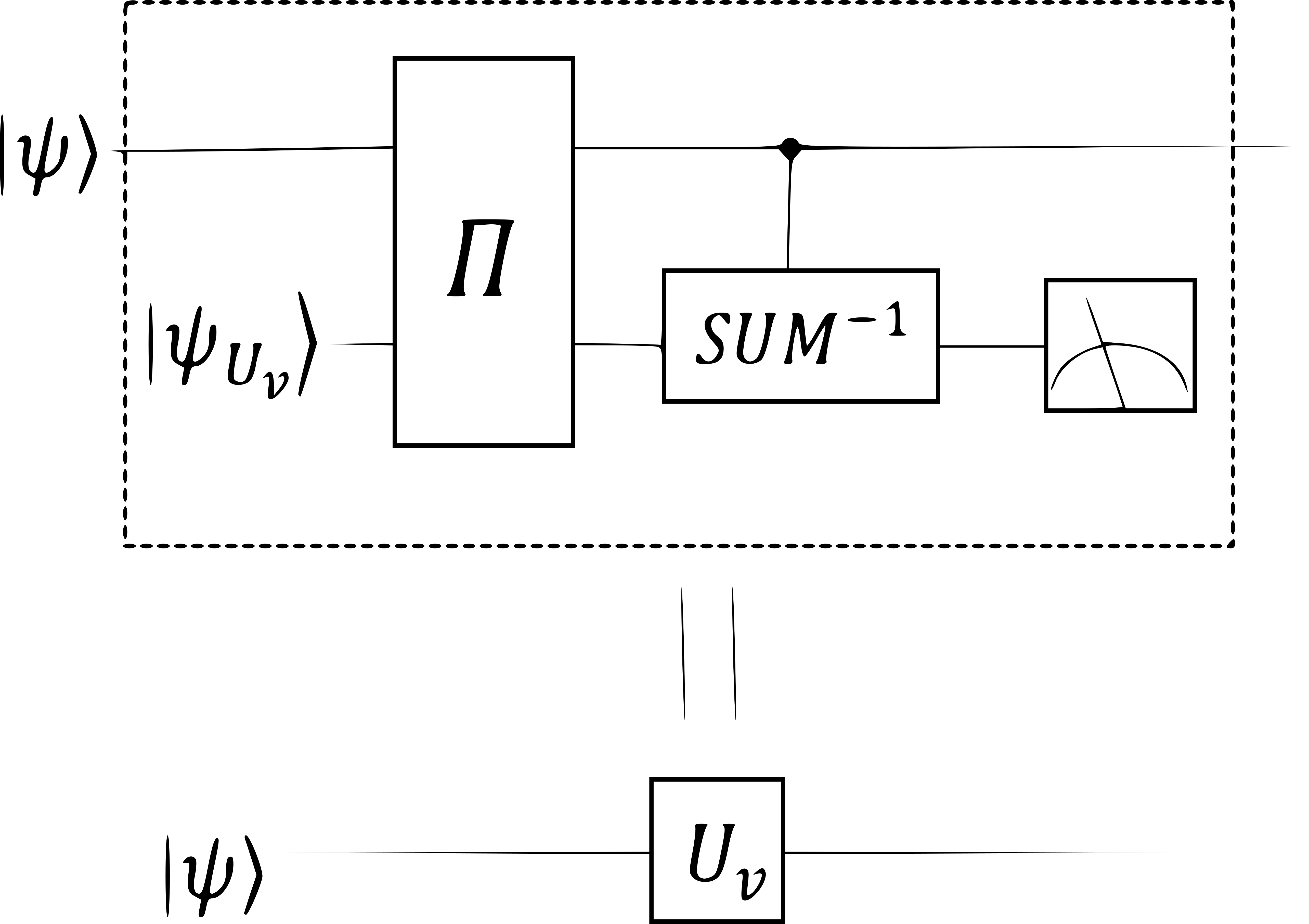
This projection is equivalent to measuring the observable to get eigenvalue 1. If we get eigenvalue , we perform a on the first qudit state to recover it back to the 1-eigenspace. In fact, this gadget works for implementing any diagonal gate by injecting the state .
Appendix E Magnitude and phase of magic state inner product with orbit representatives of nonorthogonal decompositions
Here we compute equation 12. We begin with . In this case we need only tabulate the inner product for three values of :
| (76) |
Giving:
| (77) |
The largest magnitude overlap is obtained for .
Now we consider general prime . Given the expression for we can write:
| (78) |
where is a cubic in given by:
| (79) |
The evaluation of cubic gauss sums is not as straightforward as for quadratic gauss sums. However, we can obtain a closed form for the phase of the sum, up to a sign, by depressing the cubic to remove the quadratic term. In this case this is particularly simple:
| (80) |
where:
| (81) |
Then:
| (82) |
The magnitude of this expression can be determined from the sum, which is real:
| (83) |
While this shows that the sum is real, it does not guarantee that it is positive, and hence the phase of the inner product, up to a sign, is given by:
| (84) |
Appendix F Canonical forms for Qudit stabilizer states and inner product algorithm
A qubit stabilizer state can be written as the following canonical form [31, 12]:
| (85) |
where is a linear form and takes the quadratic form . s, s are constants in . is an affine space defined as , with being a matrix with entries in .
To prove this canonical form holds true for all qubit stabilizer states, one only need to make sure that every state in this form is the eigenstate of a stabilizer operator, as shown in [12]. It also suffices to verify that any of the gates preserves the form, only changing the coefficients of , and affine space . This proof is given in [31].
The normal form was generalized to arbitrary dimensions in [19]. The stabilizer canonical form for qudits is:
| (86) |
where . The state has support in an -dimensional affine space
| (87) |
is an matrix and has each of its columns being with binary entries, while is a vector that has entries in . The division of the phase into two quadratic terms reflects the action of the phase and Hadamard gates, respectively. States of this form were shown to be the eigenstate of some Pauli (Weyl-Heisenberg) operator in [19].
This quadratic form on the exponent can also be represented in matrix form:
| (88) |
where is taken modulo . Here is a matrix with its diagonal terms being and off-diagonal terms being and is a matrix where each term corresponds to .
We will give a new proof that this form is preserved under Clifford operations using the properties of quadratic Gauss sums. We give this proof in order to develop the techniques we will use in the inner product algorithm for qudit stabilizer states.
We consider the single qudit case first. We will prove that the form:
| (89) |
is preserved under the action of the single-qudit Clifford generators where and belong to , is a shift vector that also belongs to . We are studying single-qudit case here so is either 0 or 1. When , this is simply a computational basis state.
Acting with diagonal Clifford gates on (89) such as or will only change the coefficients and in this expression. Similarly, acting with powers of the gate will only shift , again preserving the quadratic form of the exponents.
It only remains to check the Hadamard gate:
| (90) |
If , the quantity in the parentheses is simply a phase factor without the sum. Then this form reverts to (89) with . If , we recognize the quantity in the parentheses as a Gauss sum. There are again two cases. If , then we have
| (91) |
Then (90) reverts to (89) as case, i.e., a computational basis state.
If , to compute this Gauss sum, we first complete the square:
| (92) |
where , meaning that and .
The value of this Gauss sum is well known:
| (93) |
where is the Legendre symbol.
Hence:
| (94) |
The new coefficients and here are still in . This means that the general form of single-qudit stabilizer states is preserved under the action of any Clifford operations.
For multi-qudit states, we have the same affine space property as the qubit case except that the additions are modulo . Before we give the proof, we need to show that quadratic form given in terms of the basis vectors of the affine space and the qudit vectors itself are equivalent. Changing the arguments only changes the coefficients of the quadratic form. Given eq.(88), we further assume the quadratic and linear matrices in terms of being and :
| (95) |
From this equation, we can see the relationship between , and , : , and .
Now we use Van den Nest’s method [31] to prove that the canonical form (86) is preserved under the action of , and . The gate shifts the affine space by mapping to , without changing the phases. As in the qubit case, we only need to add the th column of the matrix to the th column:
| (96) |
differs from by .
Acting with on qudit results in the state:
| (97) |
which again leaves the canonical form unchanged.
The Hadamard gate requires some work. Without loss of generality, we assume that acts on the first qudit:
| (98) |
where is the first row of and is the rest of it. If is still full rank after taking out , we obtain the new to be:
| (99) |
Therefore we have basis vectors now, and becomes the new . The term in the phase can be absorbed in the quadratic form . So this is of the canonical form (86).
If is rank after taking out , then the columns of are not linearly independent. In this case one of the s is redundant and we want it to be summed out in order to get back to the canonical form. Without loss of generality, let’s assume that , therefore . If we denote for to () and , and can be written in terms of with different coefficients from and , say and , together with some constant factor which can be neglected. Then eq.(98) becomes:
| (100) |
Here the parenthesis contains the Gauss sum we computed earlier. Then we can drop the prime for the s and absorb the result of the Gauss sum and into the and functions. Finally we arrive at the same form but with different coefficients. Hence, the canonical form is preserved under the action of all Clifford gates.
We now use this canonical form and the Gauss sum techniques to provide an algorithm for the computation of the inner products of two qudit stabilizer states.
F.1 The inner product of two qudit stabilizer states
The inner product between two qubit stabilizer states can be computed efficiently in ([1, 15, 10, 8]). However, a corresponding algorithm for qudits has not yet been given, although most aspects of the theory of stabilizer states have been generalized [16, 19]. We will now describe a algorithm that computes the inner product of two qudit stabilizer states based on the Gauss sum techniques we discussed in the previous section.
As discussed above, the quadratic form in terms of the basis vector of the affine space and the qudit vector itself are equivalent. Therefore eq. (86) is equivalent to the following:
| (101) |
where is the affine space defined by in eq.(87).
Assume we have two qudit stabilizer states and , which take the above form (101) with subindices 1 and 2:
| (102) |
where , , , is the dimension of and is the quadratic form in the new basis of . The new basis of the affine space , as well as the new quadratic form associated with it, can be calculated with the same method used by Bravyi and Gosset in Appendix , for qubits [8], with cost .
What remains in eq.(102) is a Gauss sum, which we again rewrite in the following form:
| (103) |
where the exponent is given by eq. (88). We can diagonalize and factor this sum into a product of Gauss sums over . We obtain a transformation matrix that gives:
| (104) |
where is the diagonal matrix with entries .
Then if we further define , we obtain
| (105) |
where . This is a product of Gauss sums, as given in eq. (92, 93, 94).
Each Gauss sum only takes time, so the product of of them takes time . The scaling of this algorithm is determined by the complexity of Gaussian elimination, because has rank . Therefore, together with the first step to obtain , the algorithm takes time overall in the worst case.
Appendix G Evaluation of
The quantity is given by eq. (16):
| (106) |
We can see that this quantity is a function of the values ,…,. We label the phase of by for all , where . Using eqn. (10) can be rewritten in the following form:
| (107) |
where is the Hamming weight of codeword in code , i.e. the number of nonzero elements in the codeword. means the number of digits in string that equals to . If we regard as a linear code, then the qubit case is exactly the weight enumerator of the code. In the qudit case, depends on the Hamming weight as well as the s. Now let’s calculate an explicit expression for the s.
For the case, we specifically obtain and . For case, we assume our initial stabilizer state . And
| (108) |
where the for Campbell’s choice of is simply according to eq.(3) and subsection C of section IV. We can calculate as
| (109) |
Therefore we can rewrite as
| (110) |
Then we can calculate as
| (111) |
This is a quadratic Gauss sum times a phase. Using eq.(92) and (93) for and , we obtain:
| (112) |
The final expression of in terms of is:
| (113) |
where again is the Legendre symbol.