Directed Random Geometric Graphs

We first prove the indegree case. Consider the probability that a vertex $v$ has indegree $k$. For this to happen, there must be exactly $k$ other vertices in $v$’s circle (of radius $r_{v}$). The probability of this is

$$P[\delta_{in}(v)=k]=\int_{r_{0}}^{1/2}P[r_{v}=r]\text{ }P[\delta_{in}(v)=k\mid r_{v}=r]\ dr.$$

(3)

Since the points are distributed uniformly on the plane, $P[\delta_{in}(v)=k\mid r_{v}=r]$ is the binomial random variable that describes the probability of exactly $k$ points lying within the volume of the $d$-dimensional sphere. This gives

$$P[\delta_{in}(v)=k]=\eta\dbinom{n}{k}\int_{r_{0}}^{1/2}\frac{1}{r^{\alpha}}(V_{d}r^{d})^{k}(1-V_{d}r^{d})^{n-k}\ dr.$$

(4)

Making the substitution $u=V_{d}r^{d}$ gives us

$$P[\delta_{in}(v)=k]=\frac{\eta}{d}\dbinom{n}{k}V_{d}^{\frac{\alpha-1}{d}}\int_{V_{d}r_{0}^{d}}^{V_{d}/2^{d}}u^{k-1-\frac{\alpha-1}{d}}(1-u)^{n-k}\ du.$$

(5)

We let $\beta=\frac{\alpha-1}{d}$ for convenience and express the integrand in terms of the exponential function obtaining

$$P[\delta_{in}(v)=k]=\frac{\eta}{d}\dbinom{n}{k}V_{d}^{\beta}\int_{V_{d}m^{d}}^{V_{d}/2^{d}}\exp\left[n\left(\frac{k-\beta-1}{n}\ln u+(1-\frac{k}{n})\ln(1-u)\right)\right]\ du.$$

Now let $f(u)=\frac{k-\beta-1}{n}\ln u+(1-\frac{k}{n})\ln(1-u)$ so that the integrand is of the form $e^{nf(u)}$. Treating $n$ as the large part and setting $f^{\prime}(u)=0$, the saddle point is $u_{sp}=\frac{k-\beta-1}{n-\beta-1}$ and

$$f^{\prime\prime}(u_{sp})=-\frac{(n-\beta-1)^{3}}{n(k-\beta-1)(n-k)}.$$

Note that for large $n$, $f^{\prime\prime}(u_{sp})$ approaches a negative constant. The steepest descent method gives (see [22])

$$P[\delta_{in}(v)=k]\approx\frac{\eta}{d}\dbinom{n}{k}V_{d}^{\beta}e^{nf(u_{sp})}\sqrt{\frac{2\pi}{n\mid f^{\prime\prime}(u_{sp})\mid}},$$

(6)

which after inserting $f(u_{sp})$ and $f^{\prime\prime}(u_{sp})$ reads

$$P[\delta_{in}(v)=k]\approx\frac{\eta}{d}\dbinom{n}{k}V_{d}^{\beta}\frac{\sqrt{2\pi}(k-\beta-1)^{k-\beta-1/2}(n-k)^{n-k+1/2}}{(n-\beta-1)^{n-\beta+1/2}}.$$

(7)

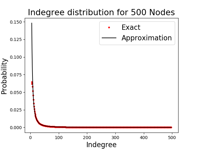
In fact, as $n\rightarrow\infty$, the two sides of Eq. (6) become asymptotically equivalent [23]. As show in figure 3, the steepest descent result gives an excellent approximation. One can ignore the term $\frac{\eta}{d}$ since it do not depend on $k$ so they only contribute to the normalizing constant for $\delta_{in}.$ We now show that for large $n$, Eq. (7) gives rise to a power law in $k$. Using Stirling’s approximation one obtains

$$\frac{1}{\sqrt{2\pi}\left(n-\beta-1\right)}\left(\frac{n}{k-\beta-1}\right)^{\beta+1}\leq\dbinom{n}{k}\frac{(k-\beta-1)^{k-\beta-1/2}(n-k)^{n-k+1/2}}{(n-\beta-1)^{n-\beta+1/2}}\leq\frac{1}{\sqrt{2\pi}\left(n-\beta-1\right)}\left(\frac{n}{k}\right)^{\beta+1}.$$

Ignoring factors that do not depend on $k$, we see that $P[\delta_{in}(v)=k]\propto k^{-\beta-1}$ as desired.

We now analyze the outdegree case. Consider a vertex $v$. $v$ has outdegree $k$ if it lies in exactly $k$ circles of other vertices. Now consider any other vertex $u\neq v$. The probability that $v$ lies inside $u^{\prime}s$ circle is given by

$$z=\int_{r_{0}}^{1/2}P[v\text{ in }u^{\prime}s\text{ ball}|r_{u}=r]\,P[r_{u}=r]\,dr,$$

where $P[v\text{ in }u^{\prime}s\text{ ball}|r_{u}=r]=V_{d}r^{d}$ and $P[r_{u}=r]=\eta/r^{\alpha}$. Note that $z$ does not depend on $v$ or $u$. Since the radii of all circles are picked independently, it follows that the probability that the outdegree of vertex $v$ is $k$ is $\binom{n-1}{k}z^{k}(1-z)^{n-k}$. One can calculate $z$ exactly to be

$$z=\int_{r_{0}}^{1/2}\frac{\eta}{r^{\alpha}}\,V_{d}\,r^{d}\ dr=\frac{\eta V_{d}}{d-\alpha+1}\left(\frac{1}{2^{d-\alpha+1}}-r_{0}^{d-\alpha+1}\right).$$

Defining $\alpha=\beta d+1$ for $\beta>1$ the above expression reads

$$z=\frac{\beta V_{d}}{\beta-1}\left(\frac{r_{0}^{\beta d}\,2^{-d}-2^{-\beta d}r_{0}^{d}}{r_{0}^{\beta d}-2^{-\beta d}}\right).$$

Using Taylor expansion, and recalling that $\beta=\frac{\alpha-1}{d}$ and $1\gg z$, the equation above reduces to

$$z=\left(\frac{\alpha-1}{\alpha-1-d}\right)\frac{\log n}{n}+\mathcal{O}\left(\frac{\log n}{n}\right)^{\beta-1}$$

and we are done. ∎

To find the total number of edges, it suffices to count all the outdegrees edges. Since there are $n-1$ nodes that $v$ can connect to with independent probabilities, Theorem 1 implies that the expected outdegree of any vertex is $\Theta(\log n)$. Hence, the total number of edges is $\Theta(n\log n)$. ∎

We note that if $u,v$ and $w$ form a type $2$ triangle then $d(w,v)\leq r_{w}$, $d(v,u)\leq r_{v},d(u,w)\leq r_{u}$. Without loss of generality, suppose that $r_{v}$ is the minimum radius: $r_{v}=\min(r_{u},r_{v},r_{w}).$ Then, we have $r_{v}\leq r_{u}$ so it follows that

$$d(v,u)\leq r_{v}\leq r_{u}.$$

Hence, there must also be a directed edge from $v$ to $u$. That is, $u,v$ and $w$ also form a type $1$ triangle, as desired. ∎

We give an abridged version of the proof. Please see the appendix for full details. Throughout the proof, $P[\cdot]$ denotes the probability of an event while $p(\cdot)$ denotes the probability density of a random variable. By linearity of expectation,

$$\mathbb{E}[|S|]=n(n-1)(n-2)\,P(v\leadsto u,w\leadsto u,v\leadsto w)$$

for randomly selected vertices $u,v,w$. Without loss of generality, we may take $u$ to be located at the origin. Then condition on the locations of $v$ and $w$, denoted by $\mathbf{x_{v}}$ and $\mathbf{x_{w}}$, as well as the radii of circles centered at $u$ and $w$, denoted by $r_{u}$ and $r_{w}$.

It is clear that the radii of circles corresponding to $u$ and $w$, along with the locations of $v$ and $w$ are independent. Additionally, edges are conditionally independent given these radii and their locations. The probability density of the points $x_{v}$ and $x_{w}$ is $1$ since $v,w$ are chosen uniformly over the unit torus: i.e. $p(\mathbf{x_{v}})=p(\mathbf{x_{w}})=1$. Furthermore, $P[v\leadsto u|\mathbf{x_{v}},r_{u}]=\mathbbm{1}[d(\mathbf{x_{v}},0)<r_{u}]$, as we draw an edge from $v$ to $u$ if and only if $\mathbf{x_{v}}$ is inside the circle of radius $r_{u}$ centered at $u$ (the origin). Similarly, $P[w\leadsto u|\mathbf{x_{w}},r_{u}]=\mathbbm{1}[d(\mathbf{x_{w}},0)<r_{u}]$. Finally, we have that $P[v\leadsto w|\mathbf{x_{w}},\mathbf{x_{v}},r_{w}]=\mathbbm{1}[d(\mathbf{x_{v}},\mathbf{x_{w}})<r_{w}]$, as we draw an edge from $v$ to $w$ if and only if the distance between their coordinates is less than the radius of $w$’s circle. Note that $\mathbbm{1}[d(\mathbf{x_{v}},\mathbf{x_{w}})<r_{w}]\leq 1$ is always true. Using these ideas, we arrive at the following inequality

$$P[v\leadsto u,w\leadsto u,v\leadsto w]\leq V_{d}^{2}\eta\int_{r_{0}}^{\frac{1}{2}}r_{u}^{2d-\alpha}=V_{d}^{2}\eta\left[\frac{r_{u}^{2d-\alpha+1}}{2d-\alpha+1}\right]^{\frac{1}{2}}_{r_{0}}.$$

As $n$ becomes large, for any fixed $d$ we have that $r_{0}$ goes to $0$. This then implies (for $\alpha>2d$) that the dominant term in the above (and a valid, asymptotically tight upper bound) is:

$$V_{d}^{2}\eta\frac{r_{0}^{2d-\alpha+1}}{\alpha-2d-1}=C_{1}\frac{\log^{2}(n)}{n^{2}}$$

where $C_{1}$ is some constant independent of $n$. Using similar reasoning as above, we can get a lower bound on $P[v\leadsto u,w\leadsto u,v\leadsto w]$. Specifically, in the appendix, it is shown that

		$\displaystyle P[v\leadsto u,w\leadsto u,v\leadsto w]\geq V_{d}^{2}\eta^{2}\int_{r_{0}}^{\frac{1}{4}}dr_{u}r_{u}^{2d-\alpha}\left(\frac{(2r_{u})^{1-\alpha}-(1/2)^{1-\alpha}}{\alpha-1}\right)$
		$\displaystyle=\frac{V_{d}^{2}\eta^{2}}{\alpha-1}\left[\frac{2^{-\alpha}\text{ }r_{0}^{2d-2\alpha-2}}{\alpha-d-1}\left(1-(4r_{0})^{2(\alpha+1)-2d}\right)-\frac{2^{\alpha-1}\text{ }r_{0}^{2d-\alpha+1}}{\alpha-2d-1}\left(1-(4r_{0})^{\alpha-1-2d}\right)\right].$

For fixed $d$, as $n$ goes to infinity, $r_{0}$ goes to $0$, so that the leading order term here is the one containing the factor $r_{0}^{2d-2\alpha-2}$ (as $\alpha>2d>d-1$). Thus, we have the lower bound

$$P[v\leadsto u,w\leadsto u,v\leadsto w]\geq(C_{2}-\epsilon)\frac{\log^{2}(n)}{n^{2}}$$

for any $\epsilon>0$, for large enough $n$. This proves that, for fixed $\alpha,d$:

$$C_{1}\frac{\log^{2}(n)}{n^{2}}\geq P[v\leadsto u,w\leadsto u,v\leadsto w]\geq(C_{2}-\epsilon)\frac{\log^{2}(n)}{n^{2}}.$$

Multiplying by $n(n-1)(n-2)$, we get:

$$C_{1}n\log^{2}(n)\geq\mathbb{E}[|S|]\geq(C_{2}-\epsilon)n\log^{2}(n)$$

for any $\epsilon$, given that $n$ is sufficiently large. This proves that $\mathbb{E}[|S|]\in\Theta(n\log^{2}(n))$, as desired. ∎

We give an abridged proof. Please see the appendix for full details. By linearity of expectation (where the expectation is over all possible DRGG), $\mathbbm{E}[\overline{C}_{\text{in}}]=\mathbbm{E}[c_{u}]$ for a randomly selected vertex $u$. Moreover,

$$\mathbbm{E}[c_{u}]=\mathbbm{E}\left[\frac{|\{v,w:v\leadsto u,w\leadsto u,v\leadsto w\}|}{d_{u}(d_{u}-1)}\right]=\sum_{k}P(d_{u}=k)\frac{\mathbbm{E}[|\{v,w:v\leadsto u,w\leadsto u,v\leadsto w\}||d_{u}=k]}{k(k-1)}$$

from the law of iterated expectation. Furthermore,

$$\mathbbm{E}[|\{v,w:v\leadsto u,w\leadsto u,v\leadsto w\}|\,|d_{u}=k]=k(k-1)P(v\leadsto w|v\leadsto u,w\leadsto u,d_{u}=k)$$

by linearity of expectation. Then, we can substitute this expression into the sum given for $\mathbbm{E}[c_{u}]$:

$$\mathbbm{E}[\overline{C}_{\text{in}}]=\sum_{k}P[d_{u}=k]P[v\leadsto w|v\leadsto u,w\leadsto u,d_{u}=k].$$

After some computation, detailed in the Appendix, one obtains:

$$\mathbbm{E}[\overline{C}_{\text{in}}]=\int dr_{u}p(r_{u})\int dr_{w}p(r_{w})\int_{||\mathbf{x_{v}}||<r_{u}}d^{d}\mathbf{x_{v}}\int_{||\mathbf{x_{w}}||<r_{u}}d^{d}\mathbf{x_{w}}\frac{\mathbbm{1}[||\mathbf{x_{v}}-\mathbf{x_{w}}||<r_{w}]}{V_{d}^{2}r_{u}^{2d}}.$$

For odd $d$, we can compute this explicitly (work detailed in the Appendix):

$$\mathbbm{E}[\overline{C}_{\text{in}}]=\frac{dd!!}{(d-1)!!}\sum_{k=0}^{\frac{d-1}{2}}\frac{(-1)^{k}}{2k+1}\dbinom{\frac{d-1}{2}}{k}\left(\frac{1}{d}\frac{(\alpha-1)^{2}}{(\alpha-1)^{2}-d^{2}}-\frac{1}{2^{2k+1}(2k+d+1)}\frac{(\alpha-1)^{2}}{(\alpha-1)^{2}-(2k+d+1)^{2}}\right).$$

(8)

For even $d$, we cannot get nice closed forms since the density function of two randomly chosen points does not have a nice form like the one that exists for odd $d$. However, we can perform asymptotic analysis and show that the clustering coefficient also approaches a constant as $n\rightarrow\infty$ for even $d$ as well. ∎

The conditional probability can be written as $\frac{P[u\leadsto v,v\leadsto u]}{P[v\leadsto u]}$. We now compute the numerator and denominator separately. As before, we can without loss of generality situate $u$ at the origin. Then,

$$P[u\leadsto v,v\leadsto u]=\int_{r_{0}}^{\frac{1}{2}}dr_{u}\int_{[0,1]^{d}}d^{d}\mathbf{x_{v}}\int_{r_{0}}^{\frac{1}{2}}dr_{v}P[u\leadsto v,v\leadsto u|r_{u},\mathbf{x_{v}},r_{v}]\cdot p(r_{u},\mathbf{x_{v}},r_{v}).$$

Since $u,v$ share an undirected edge if and only if their separation is less than the radii of both of their circles, we have

$$P[u\leadsto v,v\leadsto u|r_{u},\mathbf{x_{v}},r_{v}]=\mathbbm{1}[d(\mathbf{x_{v}},0)<r_{u}]\mathbbm{1}[d(\mathbf{x_{v}},0)<r_{v}]$$

Moreover, $p(r_{u},\mathbf{x_{v}},r_{v})=p(r_{u})p(\mathbf{x_{v}})p(r_{v})$ as each of these $3$ quantities is chosen independently. Then, the integral is rewritten:

$$\int_{||\mathbf{x_{v}}||<\frac{1}{2}}d^{d}\mathbf{x_{v}}\int_{||\mathbf{x_{v}}||}^{\frac{1}{2}}dr_{u}p(r_{u})\int_{||\mathbf{x_{v}}||}^{\frac{1}{2}}dr_{v}p(r_{v})=\int_{||\mathbf{x_{v}}||<\frac{1}{2}}d^{d}\mathbf{x_{v}}P[r_{u}>||\mathbf{x_{v}}||]P[r_{v}>||\mathbf{x_{v}}||].$$

The integrand only depends on the norm of $\mathbf{x_{v}}$; we use spherical coordinates to write it as:

$$S_{d-1}\int_{0}^{\frac{1}{2}}r^{d-1}P[r_{u}>r]P[r_{v}>r]dr$$

where $S_{d-1}=\frac{2\pi^{d/2}}{\Gamma(\frac{d}{2})}$. We can split this integral into portions that go from $0$ to $r_{0}$, where $P[r_{u}>r]$ and $P[r_{u}>r]$ each evaluate to $1$, and a portion going from $r_{0}$ to $\frac{1}{2}$. By direct computation and for $b\geq r_{0}$, one obtains

$$\int_{b}^{\frac{1}{2}}drp(r)=\frac{\eta}{\alpha-1}\left(\frac{1}{b^{\alpha-1}}-2^{\alpha-1}\right),$$

and we have

$$P[u\leadsto v,v\leadsto u]=S_{d-1}\left[\frac{r_{0}^{d}}{d}+\frac{\eta^{2}}{(\alpha-1)^{2}}\int_{r_{0}}^{\frac{1}{2}}r^{d-1}\left(\frac{1}{r^{\alpha-1}}-2^{\alpha-1}\right)^{2}dr\right].$$

We are interested in the behavior of this integral as $n\to\infty$, or equivalently $r_{0}\to 0.$ Therefore, for sufficiently large $n$,

$$\int_{r_{0}}^{1/2}r^{d-1}\left(\frac{1}{r^{\alpha-1}}-2^{\alpha-1}\right)\ dr=\frac{r_{0}^{d-2\alpha+2}}{2\alpha-d-2}+\mathcal{O}(r_{0}^{d-\alpha+1})+C$$

for some constant $C$. Using the Taylor expansion of $\eta$ around $0$ and noting that $\alpha>d+1$ (see III), we get

$\displaystyle P[u\leadsto v,v\leadsto u]$

$\displaystyle=S_{d-1}\left(\frac{r_{0}^{d}}{d}+\frac{r_{0}^{d}}{2\alpha-d-2}\right)+\mathcal{O}(r_{0}^{d+\alpha-1}).$

∎

First consider three vertices $w_{1},w_{2}$ and $w_{3}$ chosen uniformly at random. If there is a directed edge from $w_{1}$ to $w_{2}$, then this does not affect the probability of an edge from $w_{2}$ to $w_{3}$. This is because once the locations of $w_{1}$ and $w_{2}$ are fixed, the location of $w_{3}$ is still uniform, and having an edge from $w_{2}$ to $w_{3}$ only depends on the location of $w_{3}$. Thus, given a length $k$ directed path from $u$ to $v$, the edges of this path are independent of one another. Hence, if $a_{k}$ denotes the expected number of directed paths of length $k$ form $u$ to $v$, we have

$$\mathbb{E}[a_{k}]=\dbinom{n-2}{k-1}z^{k}(k-1)!$$

(9)

where $z$ is the probability of an edge in $G(n,\alpha,d)$ which is given by $\frac{C\log n}{n}$ (Theorem 1) where $C=\frac{\alpha-1}{\alpha-1-d}$. Taking $n$ large, shifting $k\rightarrow k+1$, and using $\binom{n}{k}\geq\frac{n^{k}}{k^{k}}$, we have

$$\mathbb{E}[a_{k}]\geq\sqrt{2\pi k}\left(\frac{C\log n}{e}\right)^{k}\,\frac{C\log n}{n}.$$

Hence, it suffices to find a $k$ such that $(\frac{\log n}{e})^{k}\geq n.$ This is equivalent to finding a $k$ such that $k\log\log n-k\geq\log n.$ Rearranging, we see that $k\geq\frac{\log n}{\log\log n}$ works for large $n$, as desired. Therefore, the expected number of paths of length $k=\frac{\log n}{\log\log n}$ is at least

$$\mathbb{E}[a_{k}]\geq C\sqrt{2\pi k}\log k\geq 1.$$

∎

References

- [1] Bin Zhang and Steve Horvath. A general framework for weighted gene coexpression network analysis. In STATISTICAL APPLICATIONS IN GENETICS AND MOLECULAR BIOLOGY 4: ARTICLE 17, 2005.
- [2] A. Capocci, V. D. P. Servedio, F. Colaiori, L. S. Buriol, D. Donato, S. Leonardi, and G. Caldarelli. Preferential attachment in the growth of social networks: The internet encyclopedia wikipedia. Phys. Rev. E, 74:036116, Sep 2006. doi: 10.1103/PhysRevE.74.036116. URL https://link.aps.org/doi/10.1103/PhysRevE.74.036116.
- [3] D. Ediger, K. Jiang, J. Riedy, D. A. Bader, and C. Corley. Massive social network analysis: Mining twitter for social good. In 2010 39th International Conference on Parallel Processing, pages 583–593, Sept 2010. doi: 10.1109/ICPP.2010.66.
- [4] M. Kaiser and C. C. Hilgetag. Spatial growth of real-world networks. Phys. Rev. E, 69(3):036103, March 2004. doi: 10.1103/PhysRevE.69.036103.
- [5] S. Boccaletti, V. Latora, Y. Moreno, M. Chavez, and D.-U. Hwang. Complex networks: Structure and dynamics. Physics Reports, 424(4):175 – 308, 2006. ISSN 0370-1573. doi: https://doi.org/10.1016/j.physrep.2005.10.009. URL http://www.sciencedirect.com/science/article/pii/S037015730500462X.
- [6] S. Tanimoto. Power laws of the in-degree and out-degree distributions of complex networks. ArXiv e-prints, December 2009.
- [7] Albert-Laszlo Barabasi and Reka Albert. Emergence of scaling in random networks. Science, 286(5439):509–512, 1999. ISSN 0036-8075. doi: 10.1126/science.286.5439.509. URL http://science.sciencemag.org/content/286/5439/509.
- [8] Robert Elsasser, Leszek Gasieniec, and Thomas Sauerwald. On radio broadcasting in random geometric graphs. International Symposium on Distributed Computing, 5218:212–226, 01 1970.
- [9] Xingde Jia. Wireless networks and random geometric graphs. In 7th International Symposium on Parallel Architectures, Algorithms and Networks, 2004. Proceedings., pages 575–579, May 2004. doi: 10.1109/ISPAN.2004.1300540.
- [10] Albert-Laszlo Barabasi, Reka Albert, and Hawoong Jeong. Scale-free characteristics of random networks: The topology of the world-wide web, 2000.
- [11] Stefan Kambiz Behfar, Ekaterina Turkina, Patrick Cohendet, and Thierry Burger-Helmchen. Directed networks different link formation mechanisms causing degree distribution distinction. Physica A: Statistical Mechanics and its Applications, 462(C):479–491, 2016. URL https://EconPapers.repec.org/RePEc:eee:phsmap:v:462:y:2016:i:c:p:479-491.
- [12] B. A. Huberman, D. M. Romero, and F. Wu. Social networks that matter: Twitter under the microscope. ArXiv e-prints, December 2008.
- [13] Mark Newman. Networks: An Introduction. Oxford University Press, Inc., New York, NY, USA, 2010. ISBN 0199206651, 9780199206650.
- [14] Duncan Watts and Steven H. Strogatz. Collective dynamics of small world networks. Nature, 393:440–2, 07 1998.
- [15] N. Durak, A. Pinar, T. G. Kolda, and C. Seshadhri. Degree Relations of Triangles in Real-world Networks and Models. ArXiv e-prints, July 2012.
- [16] B. Bollobas. Mathematical results on scale-free random graphs. In Handbook of Graphs and Networks, pages 1–37. Wiley, 2003.
- [17] Jesper Dall and Michael Christensen. Random geometric graphs. Phys. Rev. E, 66:016121, Jul 2002. doi: 10.1103/PhysRevE.66.016121. URL https://link.aps.org/doi/10.1103/PhysRevE.66.016121.
- [18] M. Bradonjic and W. Perkins. On Sharp Thresholds in Random Geometric Graphs. ArXiv e-prints, August 2013.
- [19] Paul Balister, Amites Sarkar, and Bela Bollobas. Percolation, Connectivity, Coverage and Colouring of Random Geometric Graphs, pages 117–142. Springer Berlin Heidelberg, Berlin, Heidelberg, 2008. ISBN 978-3-540-69395-6. doi: 10.1007/978-3-540-69395-6_2. URL https://doi.org/10.1007/978-3-540-69395-6_2.
- [20] Carl P. Dettmann and Orestis Georgiou. Random geometric graphs with general connection functions. Phys. Rev. E, 93:032313, Mar 2016. doi: 10.1103/PhysRevE.93.032313. URL https://link.aps.org/doi/10.1103/PhysRevE.93.032313.
- [21] Eric W. Weisstein. "pareto distribution." from mathworld–a wolfram web resource. http://mathworld.wolfram.com/ParetoDistribution.html, 2018.
- [22] Richard Chapling. Asymptotic methods, April 2016.
- [23] A. Erdelyi. Asymptotic Expansions. Dover Books on Mathematics. Dover Publications, 1956. ISBN 9780486603186. URL https://books.google.com/books?id=aedk-OHdmNYC.
- [24] G. Fagiolo. Clustering in complex directed networks. Phys. Rev. E, 76(2):026107, August 2007. doi: 10.1103/PhysRevE.76.026107.
- [25] Benjamin Tabak, Marcelo Takami, J. Rocha, and Daniel Cajueiro. Directed clustering coefficient as a measure of systemic risk in complex banking networks. Working Papers Series 249, Central Bank of Brazil, Research Department, 2011. URL https://EconPapers.repec.org/RePEc:bcb:wpaper:249.
- [26] Mohammad Al Hasan and Vachik S. Dave. Triangle counting in large networks: a review. Wiley Interdisciplinary Reviews: Data Mining and Knowledge Discovery, pages e1226–n/a, 2017. ISSN 1942-4795. doi: 10.1002/widm.1226. URL http://dx.doi.org/10.1002/widm.1226. e1226.
- [27] N. Meghanathan. A random network model with high clustering coefficient and variation in node degree. In 2015 8th International Conference on Control and Automation (CA), pages 54–57, Nov 2015. doi: 10.1109/CA.2015.20.
- [28] Schreiber Nelson, McEvoy. The university of south florida word association, rhyme, and word fragment norms. http://www.usf.edu/FreeAssociation/, 1998.
- [29] Christiane Fellbaum. WordNet. Springer, 2010.
- [30] Zhibiao Wu and Martha Palmer. Verb semantics and lexical selection. CoRR, abs/cmp-lg/9406033, 1994. URL http://arxiv.org/abs/cmp-lg/9406033.
- [31] Saleh Soltan, Alexander Loh, and Gil Zussman. A learning-based method for generating synthetic power grids. 2017.
- [32] S.-J. Tu and E. Fischbach. Random distance distribution for spherical objects: general theory and applications to physics. Journal of Physics A Mathematical General, 35:6557–6570, August 2002. doi: 10.1088/0305-4470/35/31/303.
- [33] Tomas Mikolov, Ilya Sutskever, Kai Chen, Greg Corrado, and Jeffrey Dean. Distributed representations of words and phrases and their compositionality. CoRR, abs/1310.4546, 2013. URL http://arxiv.org/abs/1310.4546.