Improving Temporal Interpolation of Head and Body Pose using Gaussian Process Regression in a Matrix Completion Setting
Abstract.
This paper presents a model for head and body pose estimation (HBPE) when labelled samples are highly sparse. The current state-of-the-art multimodal approach to HBPE utilizes the matrix completion method in a transductive setting to predict pose labels for unobserved samples. Based on this approach, the proposed method tackles HBPE when manually annotated ground truth labels are temporally sparse. We posit that the current state of the art approach oversimplifies the temporal sparsity assumption by using Laplacian smoothing. Our final solution uses : i) Gaussian process regression in place of Laplacian smoothing, ii) head and body coupling, and iii) nuclear norm minimization in the matrix completion setting. The model is applied to the challenging SALSA dataset for benchmark against the state-of-the-art method. Our presented formulation outperforms the state-of-the-art significantly in this particular setting, e.g. at 5% ground truth labels as training data, head pose accuracy and body pose accuracy is approximately 62% and 70%, respectively. As well as fitting a more flexible model to missing labels in time, we posit that our approach also loosens the head and body coupling constraint, allowing for a more expressive model of the head and body pose typically seen during conversational interaction in groups. This provides a new baseline to improve upon for future integration of multimodal sensor data for the purpose of HBPE.
1. Background
Pose estimation has been a popular subject of interest within the computer vision community. While deep learning based state-of-the-art pose estimation methods (Güler et al., 2018; Wei et al., 2016; Toshev and Szegedy, 2014; Tompson et al., 2014) have achieved remarkable results in articulated pose estimation (i.e. detection and prediction of the location of body parts and joints), pose estimation remains challenging particularly for crowded scenes in the surveillance setting. Hence, it is limited to only head and body pose estimation (HBPE). Despite the seeming simplification of the task, challenges of HBPE in this particular setting (Hu et al., 2004) include but are not limited to low resolution, low light visibility, background clutter and occlusions (see Figure 1 for example).

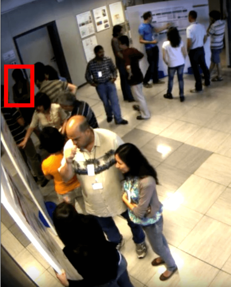


HBPE is traditionally a vision-only task. But to tackle these challenges, researchers can leverage on a multi-view camera and multi-sensor scenario (Alameda-Pineda et al., 2016). The multi-view camera setting provides multiple perspectives of people in the scene to acquire better HBPE. More interestingly, wearable sensors such as microphones, infrared or bluetooth proximity sensors, etc. have shown an ability to recover HBPE independent from the video modality (Kok et al., 2017). Additionally, they can provide more fine-grained information of the human subjects that would not otherwise be available from video only. More specifically, studying small group interactions in crowded space can benefit from data of multiple modalities (Gatica-Perez, 2009). In combination with video, these wearable sensors provide a multimodal platform to study detailed and rich information about the human subjects by complementing and enhancing HBPE, which is particularly crucial to the analysis of group and crowd behavior.
Even though it would be ideal to combine multiple modalities, wearable sensors such as microphones and infrared proximity sensors which have previously been used to study group interaction and behavior, are significantly less reliable and noisier compared to surveillance video footage for the purpose of HBPE. Another problem is that malfunctions of wearable sensors are more difficult to notice compared to those of video cameras, especially during real-time data collection where there may be visual confirmation of camera functionality but not of wearable sensor data. Due to the difficulties of working with wearable sensors, the resulting data can be either partial or entirely missing (Higger et al., 2013). Given that working with a patchwork of multimodal data can be hard, in this paper, we exploit them as part of an initialization step and focus on the problem of interpolating between sparse labels.
The setting of this study is that: i) there is a relatively small number of head and body pose samples () for each subject, ii) we want to predict pose labels for unobserved samples only using a very small number () of sparsely distributed ground truth labels, and iii) we want to take advantage of the temporal structure within the pose label data. A deep learning based method that takes into account this setting will perform sub-optimally due to small number of training samples, and also require extensive computational power and hyperparameter tuning. On the other hand, a matrix completion based transductive learning method which is more explainable and less computationally expensive, addresses the problem setting adequately. Inspired and building upon previous work by Alameda-Pineda et al. (2015), the contributions of this study are: i) an enhanced temporal smoothing scheme based on Gaussian process regression for label propagation, and ii) a more interpretable person-wise pose label prediction implementation in the transductive setting using matrix completion.
2. Related work
Head pose estimation (HPE) and body pose estimation (BPE) have been primarily studied by the computer vision community (Sigal, 2014). While impressive results could be achieved using end-to-end deep learning architectures when data capturing frontal faces (Murphy-Chutorian and Trivedi, 2009) or the full body (Cao et al., 2017), HPE and BPE remain to be challenging tasks when dealing with wide angle surveillance, with low resolution, heavy occlusions of targets, and cluttered backgrounds. The problem is often reduced to an 8-class classification problem (dividing into eight sectors), though formulating HBPE as a regression problem (Varadarajan et al., 2018) or being able to reduce coarseness in estimations can provide more meaningful information for higher level social tasks, such as predictions of social attention direction (Massé et al., 2017) and personality traits (Subramanian et al., 2013). Pioneering work (Sigal and Black, 2006; Ba and Odobez, 2009; Chen et al., 2011a) in HPE and BPE saw first successes of these tasks based on probabilistic frameworks (e.g. dynamic Bayesian networks, hidden Markov models, etc.). Due to the physical constraint of relative head and body pose and a person’s direction of movement, one line of work focuses on the joint estimation of head and body pose to achieve improved results (Chen et al., 2011a). Overall, there are more previous works on HPE compared to BPE in the surveillance and crowded space setting. In this particular setting, human heads can be more easily seen and HPE typically already contains rich enough information for high level tasks (Ba and Odobez, 2009). On the other hand, humans bodies are usually occluded because of the camera angle from the top, which makes it more difficult to predict body orientations without side information such as walking direction, etc. In contrast, HBPE in other contexts such as AR/VR video gaming, sports, etc. where full body poses data are captured by frontal view camera, is much more well-studied and can be represented by a considerable number of work (e.g. (Cao et al., 2017),(Insafutdinov et al., 2016)). Additionally, the line of works on low-resolution HPE leverages on multi-view surveillance images. Hasan et al. (2018) have recently proposed a noteworthy deep learning method based on Long Short Term Memory (LSTM) neural networks to jointly forecast trajectories and head poses. This work points to the possibility of utilizing LSTM models in predicting head and body pose sequences, which is more informative compared to solving HPE and BPE in a classification setting using Convolutional Neural Networks (CNN) (Lu et al., 2016).
In this paper, we propose to use matrix completion for HBPE, which was first proposed by Alameda-Pineda et al. (2015). This approach combines head and body visual features, inferred head orientation labels from audio recordings, body orientation labels from infrared proximity sensors, and manually annotated labels of some but not all frames. To reduce the manual effort of annotating the head pose, labels were only created every 3 seconds. Alameda-Pineda et al. poses the estimation of head and body orientations as a matrix completion problem where the visual features and labels from either wearable sensors or manual annotations are concatenated into a heterogeneous matrix, for head and body respectively. Due to sparsity and noise in the data extracted from the wearable sensors, the underlying challenge is to construct a matrix that is temporally smooth; and that is consistent with the manual annotations, the observed wearable sensor readings, and the physical constraints that tend to couple the head and body behaviour together.
3. Our Approach
The scope of the study is to jointly predict head and body pose labels as an 8-class classification problem (dividing into eight sectors) in a matrix completion transductive learning setting. Before performing HBPE, upstream processes such as multi-person detection and tracking in videos, head and body localization, and appearance-based visual feature extraction are carried out as outlined in Figure 2 (Chen et al., 2011a; Alameda-Pineda et al., 2015).

The construction of a matrix consisting of visual features and manually annotated labels is illustrated in Figure 3. Head pose features and labels are arranged into one such matrix, and similarly for body pose features and labels. Head and pose labels of each participant (independent of other participants) are estimated by completing their head and body matrices jointly. The technical core of constructing such matrices for HBPE and jointly completing the head and body matrices using our formulation is discussed in Section 4, followed by details on experimental conditions pertaining to the upstream processes (see blue modules in Figure 2) in Section 5.

4. Methodology
In the supervised learning setting for a linear classifier, the objective is to learn the weight matrix , which maps the -dimensional features space to the -dimensional (number of classes) output space where denotes the number of samples in time, by minimizing the loss on a training set as
| (1) |
When dealing with noisy features and fuzzy labels, previous research by Goldberg et al. (2010); Cabral et al. (2011); Bomma and Robertson (2015) have empirically shown the practicality of casting a classification problem into a transductive learning setting such as matrix completion. To that purpose, borrowing from the linear classifier setting, a heterogeneous matrix can be built by concatenating the pose labels , visual features , and a row of ’s (to model for bias) as
| (2) |
where . Note that is a vectorized one hot representation of pose labels.
In the HBPE setting, the duration that we are interested in predicting the pose estimations for is indicated by and this is represented by arranging samples column-wise for temporal consistency. The number of pose classes possible is denoted by . Dividing into eight sectors means that there are eight possible classes and each pose belongs to one of the eight classes. For example, a pose angle between and would be indicated by the vector . The head and body label matrices are denoted by and respectively. The feature matrices and contain the visual features from head and body crops of each person, where and denote the respective feature dimensionality. Following the definition in (2), the heterogeneous matrices are and for head pose and body pose estimation respectively. In addition, a projection matrix is introduced to extract only the head pose labels from the heterogeneous matrix . In a similar manner, a projection matrix is defined to extract body pose labels.
Matrix completion is an iterative method that attempts to fill in missing entries in a matrix, which in our context correspond to unobserved pose labels. For the purpose of the iterative scheme, the unobserved pose labels can either be initialized by side information provided by external sources, or simply set to zeros. In this study, we take the first option by initializing the unobserved samples by sensor data. The initial matrices for head and body poses are denoted by and respectively. The label matrix in , denoted by , is further divided into a training set and a test set . Similarly, the label matrix in , denoted by , is divided into and . Each training set consists of observed labels, while the test set consists of unobserved labels. The training set and test set samples are interleaved, as shown in Figure 3. In this study, training set labels are sampled from manual annotations and test set labels are initialized by sensor data, in the hope of achieving faster convergence. For the sake of brevity, the subsequent discussion will be explained for the head pose matrix. The body pose matrix and its corresponding optimization formulation are analogous to those of the head pose matrix.
The following discussion outlines the proposed matrix completion method based on the aforementioned setting. The proposed method consists of three components: i) nuclear norm minimization, ii) temporal smoothing, and iii) head-body coupling.
4.1. Nuclear norm minimization
Following the linear classifier assumption from (2), Goldberg et al. (2010) have shown that the matrix should be low rank. More concretely, the objective is to recover the missing pose labels such that the rank of the heterogeneous matrix is minimized. Rank minimization is a non-convex problem (Goldberg et al., 2010). However, Candes and Tao (2010) showed that can be relaxed to its convex envelope which is the nuclear norm, , i.e.
| (3) |
The optimization problem then becomes a minimization of the nuclear norm of .
4.2. Temporal smoothing
If samples in the heterogeneous matrix are temporally sorted, one can take advantage of the temporal structure between the columns. Pose labels are to a certain extent, temporally smooth, as poses are not expected to change drastically within a short time period. This can be seen as a column-wise regularization. Using the training set , an interpolated time series of pose labels can be generated using an appropriate interpolation scheme to estimate the unobserved pose labels entirely based on temporal consideration. In the proposed method, Gaussian process regression (GPR) is chosen as the interpolation scheme. Also known as Kriging, GPR has the same objective as other regression methods, which is to predict a value of a function at some point using a combination of observed values at other points. Rather than curve fitting using a polynomial function for instance, GPR assumes an underlying random process, more specifically a Gaussian process distribution (Bachoc et al., 2017), from which the observed values are sampled. A new posterior distribution is computed based on the assumed (Gaussian process) prior and Gaussian likelihood functions (Williams, 1998). The Gaussian process prior is characterized by a covariance function which measures the similarity between data points; and thus the choice of a suitable covariance function is an essential component in GPR. For the purpose of this study, the covariance function is chosen to be the popular Radial-Basis Function (RBF) kernel. More details of Gaussian processes and Kriging can be found in (Rasmussen and Williams, 2005).
Following this procedure, we denote as the label matrix where the missing values are imputed by the prediction of GPR. After acquiring the interpolated labels, a new matrix is defined as
| (4) |
A squared loss term is introduced into the nuclear norm minimization problem for regularization to ensure that the predicted labels do not deviate drastically from the labels obtained as a result of temporal interpolation. The projection matrix ensures that the loss is only considered over the pose labels.
Note that GPR is an example of a regression method that works well in this setting. Alternative regression methods such Laplacian smoothing (Alameda-Pineda et al., 2015), piece-wise linear interpolation and polynomial regression can also be applied. Our justification of this choice follows in the discussion section in Section 7.
4.3. Head and body coupling
So far the formulation details the manipulation of HPE and BPE matrices separately. In this section we jointly consider the two matrices as they are related. Previous research by Chen et al. (2011b); Alameda-Pineda et al. (2015); Varadarajan et al. (2018) has shown that coupling HPE and BPE is advantageous for improving accuracy. The proposed formulation also captures the physical constraints between head and body poses. Since head and body pose are jointly estimated, this relation fits in nicely as an additional regularization to the optimization problem. It is reasonable to model that head and body poses cannot be too different at any given time step. Though hinge loss would probably be more appropriate, the relation can also be captured by squared loss, for the ease of analytical derivation and numerical optimization. The regularization term can therefore be written as .
4.4. Optimization problem
To summarize, the entire optimization problem, considering all the regularizations and indicating terms associated with both head and body (described in Section 4.1-4.3) is given by
| (5) | ||||
where , , , , and are weights that control the trade-off between the different terms. The equation in (5) can be solved iteratively by an adapted Alternating Direction Method of Multipliers (ADMM) proposed by Boyd et al. (2011) and Alameda-Pineda et al. (2015) to jointly solve the minimization problem for the head and body pose matrices. We adopt the aforementioned algorithm that starts with the construction of the augmented Lagrangian, similar to the classical ADMM (Eckstein and Yao, 2012). The augmented Lagrangian of the optimization problem in (5) is given by
| (6) | ||||
where and are auxiliary variables that allow the decoupling of the optimization of and ; and and are Lagrange Multiplier matrices. The inner product of the two terms is denoted by . The update rules are similar to those of the ADMM with scaled dual variables (Boyd et al., 2011). In this context, the update rules at the -th iteration are given by
| (7) | ||||
| (8) | ||||
5. Experimental Setup
This section provides a brief introduction of the SALSA dataset that was used to obtain the experimental results, and an overview of the experimental conditions.
5.1. SALSA Dataset
The SALSA dataset is captured at a social event that consists of a poster presentation session and a mingling event afterwards, involving 18 participants. It is a multimodal dataset that includes video recordings from a multi-view surveillance camera (4 cameras) network, binary proximity sensor data acquired from sociometric badges worn by the participants, and audio recordings of each participant acquired by a microphone embedded in the sociometric badges. For this study, we only focus on the video recordings of the poster presentation session. Ground truth labels of head and body pose of each participant were manually annotated every 3 seconds. There are in total 645 ground truth annotations for each head and body pose of each participant. The authors of (Alameda-Pineda et al., 2015) also inferred head pose from microphone data and body pose from infrared proximity sensor data, independent from the video modality. These are considered as "soft" labels and further details of their extraction can be found in (Alameda-Pineda et al., 2015) and are provided as part of the dataset.
5.2. Experimental Conditions
We used the provided Histogram of Gradients (HOG) visual features for head and body crops of each participant from the SALSA dataset poster session (Alameda-Pineda et al., 2015). Similar to Alameda-Pineda et al. (2015)’s approach, visual features from the four cameras are concatenated and PCA was performed to keep 90% of the variance. This results in a 100 dimensional feature vector. Training data are the observed labels and test data are the unobserved labels to be predicted. In a transductive learning setting, it is conventional to have both the training data and test data available during training. Because the objective is to predict labels for the unobserved entries only and not generalize to further unseen data, weights are not explicitly learned. Training data and test data partitions are defined by a random projection mask to simulate random sampling over labels. Because of this randomness, training and test data are interleaved and we take advantage of this inherent structure in our formulation. Note that because of the same reason, all our experiments are conducted 10 times and results are averaged to mediate the random projection mask causing overestimation or underestimation of prediction accuracies. Additionally, the sample diversity (i.e. class distribution) is different among participants. Hence, a randomly created projection mask is rejected if it results in low sample diversity in the training set. The hyper-parameters in (6) are optimized using Bayesian optimization with 5-fold cross validation.
5.3. Implementation Details
Similar to the authors of (Alameda-Pineda et al., 2015), we assume visual features from each participant are available at any given time step. Unlike in previous approach (Alameda-Pineda et al., 2015) where the inferred "soft" labels are used as part of the training set, our experiments only use samples that were manually annotated to construct the training set. It is unclear if the experiments reported by Alameda-Pineda et al. (2015) used additional unlabeled samples along with the manual annotations and "soft" labels in their model during training.
Since we were not able to clarify ambiguities in the description of the experimental setup in the former formulation (Alameda-Pineda et al., 2015), we made the following decisions regarding the experimental setting. In this study, we construct the training and test sets from only samples that are manually annotated in the SALSA dataset. Since the quality of the "soft" labels was not quantitatively assessed by Alameda-Pineda et al. (2015), in our case, it also makes sense for us to avoid training using "soft” labels so we can more clearly see the effect of our proposed approach independently of the influence of training with weak labels. In our experiments, although "soft" labels are not considered as part of the observed samples, they are only used as initializations of unobserved samples in order to reach faster convergence. Note that columns of the matrix which are initially populated with soft labels are subject to immediate changes after being fed as inputs to the optimization problem.
6. Results
The heterogeneous matrix for head and body are initialized with the same fraction of ground truth labels as training data, though their respective random projection masks are different. Figure 4 shows the test accuracy, which is the prediction accuracy over unobserved labels, against different fractions of manual annotation used for training. The proposed method is compared against the state-of-the-art matrix completion based HBPE method by Alameda-Pineda et al. (2015). As shown in Figure 4, the proposed method is drastically superior compared to the state-of-the-art matrix completion by Alameda-Pineda et al. (2015), especially at very low fraction of manual annotations.
The difference in performance of both methods is accredited to a simple numerical phenomenon. One of the major differences between the proposed method and the method by Alameda-Pineda et al. (2015) is the temporal smoothing scheme. In the latter, the authors employed Laplacian smoothing to ensure temporal consistency over the pose estimates. While it is a reasonable choice for smoothing based on local information, GPR in contrast provides smoothing by exploiting a more global context based on only a few data points. By fitting sparse data points in the functional space, GPR is known to better recover nonlinear patterns and longer timescale trends compared to polynomial interpolation, and especially Laplacian smoothing. As a result, it provides a good accuracy even when only 5 % of the manual labels are available as training data. Additionally, person-wise HBPE results for all 18 participants at 5 % manual annotation using the two methods is reported in Table 1.
|
MC-HBPE[2] | Proposed |
| |||||||
|---|---|---|---|---|---|---|---|---|---|---|
| HPE mean (std) | BPE mean (std) | HPE mean (std) | BPE mean (std) | Head | Body | |||||
| Person 1 [119] | 0 (0) | 0 (0) | 0.49 (2.9e-2) | 0.57 (5.1e-2) | 1.19 | 1.14 | ||||
| Person 2 [132] | 0.06 (2.3e-3) | 0 (0) | 0.39 (1.0e-2) | 0.84 (1.8e-2) | 1.32 | 0.48 | ||||
| Person 3 [140] | 0.63 (3.0e-2) | 0.67 (4.1e-2) | 0.77 (1.9e-2) | 0.82 (3.2e-2) | 1.51 | 1.29 | ||||
| Person 4 [169] | 0.02 (1.6e-3) | 0.01 (3.5e-3) | 0.85 (3.6e-2) | 0.86 (2.7e-2) | 1.20 | 1.10 | ||||
| Person 5 [177] | 0.13 (2.9e-3) | 0.13 (1.2e-2) | 0.53 (5.4e-2) | 0.60 (6.1e-2) | 1.84 | 1.79 | ||||
| Person 6 [180] | 0.44 (1.6e-2) | 0.39 (1.7e-2) | 0.65 (4.0e-2) | 0.75 (4.6e-2) | 1.72 | 1.56 | ||||
| Person 7 [216] | 0.17 (6.6e-2) | 0.17 (3.1e-2) | 0.56 (3.3e-2) | 0.48 (7.5e-2) | 1.77 | 1.90 | ||||
| Person 8 [238] | 0.01 (5.2e-4) | 1.5e-4 (5.2e-4) | 0.82 (1.1e-2) | 0.88 (2.3e-2) | 0.60 | 0.37 | ||||
| Person 9 [241] | 0.34 (4.1e-3) | 0.57 (4.9e-3) | 0.63 (7.7e-2) | 0.70 (6.9e-2) | 1.57 | 1.59 | ||||
| Person 10 [261] | 0.09 (2.6e-3) | 0.12 (2.8e-3) | 0.69 (1.6e-2) | 0.85 (2.9e-2) | 1.39 | 1.21 | ||||
| Person 11 [262] | 0.13 (1.4e-3) | 0.01 (1.7e-3) | 0.60 (4.7e-2) | 0.69 (5.6e-2) | 1.56 | 1.50 | ||||
| Person 12 [267] | 0.13 (6.8e-3) | 0.03 (8.4e-3) | 0.81 (1.9e-2) | 0.82 (1.8e-2) | 1.01 | 0.96 | ||||
| Person 13 [286] | 0 (0) | 0 (0) | 0.68 (2.4e-2) | 0.75 (3.7e-e) | 1.66 | 1.60 | ||||
| Person 14 [307] | 0.09 (2.7e-2) | 0.12 (3.7e-2) | 0.37 (4.4e-2) | 0.46 (7.7e-2) | 1.88 | 1.79 | ||||
| Person 15 [313] | 0 (0) | 0 (0) | 0.57 (6.0e-2) | 0.65 (4.7e-2) | 1.16 | 1.06 | ||||
| Person 16 [350] | 0.03 (2.7e-3) | 0.03 (2.9e-2) | 0.69 (7.6e-2) | 0.69 (7.0e-2) | 1.23 | 1.23 | ||||
| Person 17 [351] | 0.13 (4.9e-2) | 0.25 (4.1e-2) | 0.52 (3.7e-2) | 0.51 (4.3e-2) | 1.74 | 1.74 | ||||
| Person 18 [353] | 0.13 (2.2e-2) | 0.20 (8.2e-3) | 0.55 (6.1e-2) | 0.72 (7.2e-2) | 1.41 | 1.12 | ||||
- •
∗ indicates the person ID encoding provided in the SALSA dataset.
During social events and in free-standing conversation groups, we expect head pose to change more than body poses and that these changes are fine-grained. Hence, it is reasonable to conclude that head poses are harder to predict compared to body poses; and it is reflected in the observation that test accuracies for head pose estimates are lower than test accuracies for body pose estimates from both the methods. This can be further analyzed by computing information entropy to illustrate the distribution of the ground truth labels used in this study. The equation for calculating entropy is given by
| (11) |
where is the information entropy measure of a set of samples and is the proportion of ground truth labels in the class. For unbiased 8 class label distribution (i.e. uniform distribution), the maximum entropy value is approximately 2.08. The entropy of head pose labels averaged over all participants is 1.43 with standard deviation 0.33. The entropy of body pose labels averaged over all participants is 1.3 with standard deviation 0.43. Therefore, head pose diversity is slightly higher than that of the body pose, which partially justifies the reasoning that head pose labels are more difficult to accurately predict than body pose labels. However, the GPR-based proposed method still manages to achieve significantly higher test accuracies for head pose estimates compared to the method by Alameda-Pineda et al. (2015).
It is worth noting that in this study, we sample training data from manual labels, whereas in the experimental setup by Alameda-Pineda et al. (2015), "soft" labels acquired from wearable devices are also used as part of training data. Experiments were also conducted where the "soft" labels provided in the dataset are included as part of the training data. However, no desirable results can be obtained. As a reference, using the same approach as that of (Alameda-Pineda et al., 2015) at 50% training data partition with 5% manual annotations and 95 % "soft" labels, we obtained 14% and 16 % for HPE and BPE respectively, compared to the reported 57% and 60% (Alameda-Pineda et al., 2015).
7. Discussion
In our proposed method, GPR performs fitting over the head and body pose estimates separately, which loosens the head and body coupling constraint to a certain extent. Though there is still point to point coupling between head pose and body pose at each time step, the head poses and body poses are each separately governed by their own trend which should be less sensitive to noise from the other. Coupling that is too tight may artificially enforce head and body pose to be the same which may not reflect the reality when it comes to small group interactions. This implicit benefit from recovering nonlinearities independently should provide rich information to study human behavior in groups.
Since wearable sensors are known to provide noisy information, not all "soft" labels can be seen to have the same quality as ground truth labels. It would be ideal to add high quality "soft" labels to training data and if they are as high quality as manual labels, they can further benefit and improve HBPE in a multimodal setting, as opposed to a single video modality. However, this prior knowledge would need to be obtained beforehand. Because the proposed formulation gives robust performance with small number of manual annotations without the use of any "soft" labels, it provides a good baseline and ground for comparison for further investigation of the quality of labels derived from wearable sensors.
While the highlight of this formulation is to predict the classification of unobserved labels based on a very small number of observed labels, the model does not extend to predicting further unseen data since the weights are not explicitly recovered. When an observed label becomes available to be included, the full model needs to be run again. One of the computational bottlenecks is Gaussian process regression, which has time complexity that makes it infeasible to scale up for large quantities of data. Another computational bottleneck is the singular value decomposition (SVD) in solving the optimization problem using ADMM (see Appendix A).
8. Conclusion
This work focuses on estimating head and body poses in crowded social scene scenario using Gaussian process regression and head and body coupling as a regularization term in a matrix completion setting. The model’s premise is to predict head and body pose labels as an 8-class classification problem in a transductive learning setting. The model is able to predict a relatively large percentage of pose labels in large continuous time segment (average 20 samples gap length, approximately 1 minute in real time) and implicitly recover the nonlinearity within the data using only a small fraction of samples as training data. The proposed model has shown to be effective on the challenging SALSA dataset and achieved desirable results of 62 % accuracy on head pose estimation and 70% accuracy on body pose estimation using only 5% of the samples as training data, showing superior performance over the state-of-the-art.
Future work on improving HBPE includes integrating wearable sensor data as regularization terms towards a truly multimodal approach. Rather than using appearance based HOG features, visual features could also be extracted using a CNN pre-trained on large image databases and fine-tuned on the SALSA dataset. Additionally, it would be interesting to assess the performance of the proposed method on different, but equally challenging datasets, such as the MatchNMingle dataset (Cabrera-Quiros et al., 2018). Further analysis of HBPE performance with respect to participants’ role in the social scenarios in question and their pose diversity may lend deeper insights to fine-grained head and body movements in group interactions.
9. Acknowledgment
The authors thank Xavier Alameda-Pineda for sharing data and implementation of his previous research (Alameda-Pineda et al., 2015).
References
- Alameda-Pineda et al. (2016) X. Alameda-Pineda, J. Staiano, R. Subramanian, L. Batrinca, E. Ricci, B. Lepri, O. Lanz, and N. Sebe. 2016. SALSA: A Novel Dataset for Multimodal Group Behavior Analysis. IEEE Transactions on Pattern Analysis and Machine Intelligence 38, 8 (Aug 2016), 1707–1720. https://doi.org/10.1109/TPAMI.2015.2496269
- Alameda-Pineda et al. (2015) Xavier Alameda-Pineda, Yan Yan, Elisa Ricci, Oswald Lanz, and Nicu Sebe. 2015. Analyzing Free-standing Conversational Groups: A Multimodal Approach. In Proceedings of the 23rd ACM International Conference on Multimedia (MM ’15). ACM, New York, NY, USA, 5–14. https://doi.org/10.1145/2733373.2806238
- Ba and Odobez (2009) Sileye O Ba and Jean-Marc Odobez. 2009. Recognizing visual focus of attention from head pose in natural meetings. IEEE Transactions on Systems, Man, and Cybernetics, Part B (Cybernetics) 39, 1 (2009), 16–33.
- Bachoc et al. (2017) F. Bachoc, F. Gamboa, J. M. Loubes, and N. Venet. 2017. A Gaussian Process Regression Model for Distribution Inputs. IEEE Transactions on Information Theory (2017), 1–1. https://doi.org/10.1109/TIT.2017.2762322
- Bomma and Robertson (2015) S. Bomma and N. M. Robertson. 2015. Joint classification of actions with matrix completion. In 2015 IEEE International Conference on Image Processing (ICIP). 2766–2770. https://doi.org/10.1109/ICIP.2015.7351306
- Boyd et al. (2011) Stephen Boyd, Neal Parikh, Eric Chu, Borja Peleato, Jonathan Eckstein, et al. 2011. Distributed optimization and statistical learning via the alternating direction method of multipliers. Foundations and Trends® in Machine learning 3, 1 (2011), 1–122.
- Cabral et al. (2011) Ricardo S. Cabral, Fernando Torre, Joao P. Costeira, and Alexandre Bernardino. 2011. Matrix Completion for Multi-label Image Classification. In Advances in Neural Information Processing Systems 24, J. Shawe-Taylor, R. S. Zemel, P. L. Bartlett, F. Pereira, and K. Q. Weinberger (Eds.). Curran Associates, Inc., 190–198. http://papers.nips.cc/paper/4419-matrix-completion-for-multi-label-image-classification.pdf
- Cabrera-Quiros et al. (2018) L. Cabrera-Quiros, A. Demetriou, E. Gedik, L. v. d. Meij, and H. Hung. 2018. The MatchNMingle dataset: a novel multi-sensor resource for the analysis of social interactions and group dynamics in-the-wild during free-standing conversations and speed dates. IEEE Transactions on Affective Computing (2018), 1–1. https://doi.org/10.1109/TAFFC.2018.2848914
- Cai et al. (2010) J. Cai, E. Candès, and Z. Shen. 2010. A Singular Value Thresholding Algorithm for Matrix Completion. SIAM Journal on Optimization 20, 4 (2010), 1956–1982. https://doi.org/10.1137/080738970 arXiv:https://doi.org/10.1137/080738970
- Candes and Tao (2010) E. J. Candes and T. Tao. 2010. The Power of Convex Relaxation: Near-Optimal Matrix Completion. IEEE Transactions on Information Theory 56, 5 (May 2010), 2053–2080. https://doi.org/10.1109/TIT.2010.2044061
- Cao et al. (2017) Zhe Cao, Tomas Simon, Shih-En Wei, and Yaser Sheikh. 2017. Realtime Multi-Person 2D Pose Estimation using Part Affinity Fields. In CVPR.
- Chen et al. (2011a) Cheng Chen, Alexandre Heili, and Jean-Marc Odobez. 2011a. Combined estimation of location and body pose in surveillance video. In Advanced Video and Signal-Based Surveillance (AVSS), 2011 8th IEEE International Conference on. IEEE, 5–10.
- Chen et al. (2011b) Cheng Chen, Alexandre Heili, and Jean-Marc Odobez. 2011b. A joint estimation of head and body orientation cues in surveillance video. In Computer Vision Workshops (ICCV Workshops), 2011 IEEE International Conference on. IEEE, 860–867.
- Eckstein and Yao (2012) Jonathan Eckstein and W Yao. 2012. Augmented Lagrangian and alternating direction methods for convex optimization: A tutorial and some illustrative computational results. RUTCOR Research Reports 32 (2012), 3.
- Gatica-Perez (2009) Daniel Gatica-Perez. 2009. Automatic Nonverbal Analysis of Social Interaction in Small Groups. Image Vision Comput. 27, 12 (Nov. 2009), 1775–1787. https://doi.org/10.1016/j.imavis.2009.01.004
- Goldberg et al. (2010) Andrew Goldberg, Ben Recht, Junming Xu, Robert Nowak, and Xiaojin Zhu. 2010. Transduction with Matrix Completion: Three Birds with One Stone. In Advances in Neural Information Processing Systems 23, J. D. Lafferty, C. K. I. Williams, J. Shawe-Taylor, R. S. Zemel, and A. Culotta (Eds.). Curran Associates, Inc., 757–765. http://papers.nips.cc/paper/3932-transduction-with-matrix-completion-three-birds-with-one-stone.pdf
- Güler et al. (2018) Riza Alp Güler, Natalia Neverova, and Iasonas Kokkinos. 2018. DensePose: Dense Human Pose Estimation In The Wild. arXiv (2018).
- Hasan et al. (2018) Irtiza Hasan, Francesco Setti, Theodore Tsesmelis, Alessio Del Bue, Fabio Galasso, and Marco Cristani. 2018. MX-LSTM: mixing tracklets and vislets to jointly forecast trajectories and head poses. arXiv preprint arXiv:1805.00652 (2018).
- Higger et al. (2013) M. Higger, M. Akcakaya, and D. Erdogmus. 2013. A Robust Fusion Algorithm for Sensor Failure. IEEE Signal Processing Letters 20, 8 (Aug 2013), 755–758. https://doi.org/10.1109/LSP.2013.2266254
- Hu et al. (2004) Weiming Hu, Tieniu Tan, Liang Wang, and S. Maybank. 2004. A survey on visual surveillance of object motion and behaviors. IEEE Transactions on Systems, Man, and Cybernetics, Part C (Applications and Reviews) 34, 3 (Aug 2004), 334–352. https://doi.org/10.1109/TSMCC.2004.829274
- Insafutdinov et al. (2016) Eldar Insafutdinov, Leonid Pishchulin, Bjoern Andres, Mykhaylo Andriluka, and Bernt Schiele. 2016. Deepercut: A deeper, stronger, and faster multi-person pose estimation model. In European Conference on Computer Vision. Springer, 34–50.
- Kok et al. (2017) Manon Kok, Jeroen D Hol, and Thomas B Schön. 2017. Using inertial sensors for position and orientation estimation. arXiv preprint arXiv:1704.06053 (2017).
- Lu et al. (2016) Yang Lu, Shujuan Yi, Nan Hou, Jingfu Zhu, and Tiemin Ma. 2016. Deep neural networks for head pose classification. In Intelligent Control and Automation (WCICA), 2016 12th World Congress on. IEEE, 2787–2790.
- Massé et al. (2017) Benoît Massé, Silèye O. Ba, and Radu Horaud. 2017. Tracking Gaze and Visual Focus of Attention of People Involved in Social Interaction. CoRR abs/1703.04727 (2017).
- Murphy-Chutorian and Trivedi (2009) Erik Murphy-Chutorian and Mohan Manubhai Trivedi. 2009. Head pose estimation in computer vision: A survey. IEEE transactions on pattern analysis and machine intelligence 31, 4 (2009), 607–626.
- Rasmussen and Williams (2005) Carl Edward Rasmussen and Christopher K. I. Williams. 2005. Gaussian Processes for Machine Learning (Adaptive Computation and Machine Learning). The MIT Press.
- Sigal (2014) Leonid Sigal. 2014. Human Pose Estimation. Springer US, Boston, MA, 362–370. https://doi.org/10.1007/978-0-387-31439-6_584
- Sigal and Black (2006) Leonid Sigal and Michael J Black. 2006. Measure locally, reason globally: Occlusion-sensitive articulated pose estimation. In Computer Vision and Pattern Recognition, 2006 IEEE Computer Society Conference on, Vol. 2. IEEE, 2041–2048.
- Subramanian et al. (2013) Ramanathan Subramanian, Yan Yan, Jacopo Staiano, Oswald Lanz, and Nicu Sebe. 2013. On the Relationship Between Head Pose, Social Attention and Personality Prediction for Unstructured and Dynamic Group Interactions. In Proceedings of the 15th ACM on International Conference on Multimodal Interaction (ICMI ’13). ACM, New York, NY, USA, 3–10. https://doi.org/10.1145/2522848.2522862
- Tompson et al. (2014) Jonathan J Tompson, Arjun Jain, Yann LeCun, and Christoph Bregler. 2014. Joint Training of a Convolutional Network and a Graphical Model for Human Pose Estimation. In Advances in Neural Information Processing Systems 27, Z. Ghahramani, M. Welling, C. Cortes, N. D. Lawrence, and K. Q. Weinberger (Eds.). Curran Associates, Inc., 1799–1807.
- Toshev and Szegedy (2014) Alexander Toshev and Christian Szegedy. 2014. DeepPose: Human Pose Estimation via Deep Neural Networks. In The IEEE Conference on Computer Vision and Pattern Recognition (CVPR).
- Varadarajan et al. (2018) Jagannadan Varadarajan, Ramanathan Subramanian, Samuel Rota Bulò, Narendra Ahuja, Oswald Lanz, and Elisa Ricci. 2018. Joint Estimation of Human Pose and Conversational Groups from Social Scenes. International Journal of Computer Vision 126, 2-4 (2018), 410–429.
- Wei et al. (2016) Shih-En Wei, Varun Ramakrishna, Takeo Kanade, and Yaser Sheikh. 2016. Convolutional Pose Machines. In The IEEE Conference on Computer Vision and Pattern Recognition (CVPR).
- Williams (1998) Christopher KI Williams. 1998. Prediction with Gaussian processes: From linear regression to linear prediction and beyond. In Learning in graphical models. Springer, 599–621.
Appendix A Derivations of ADMM
To separate head and body expressions, at iteration, the optimization problem (7) can be split into
| (12) |
and
| (13) |
Simplifying and manipulating (12), we obtain
| (14) | ||||
Equation (14) can be arranged as
| (15) |
The last term in Equation (15) results in a scalar constant and does not affect the nature of optimization. The solution to minimization problem (15) was derived by Cai et al. (2010) and Alameda-Pineda et al. (2015), and is given by
| (16) |
where the , , and are obtained from singular value decomposition (SVD) of matrix
| (17) |
and where the shrinkage operator is given by
| (18) |
and is applied element-wise to the diagonal matrix of singular values . The derivations can be similarly extended for body pose estimation matrix and the solution is given by
| (19) |
For the second step in the optimization problem (8), we define the row-vectorization form of the matrices and as and respectively. The row vectorization notation extends to other matrices in (8) similarly. Derivatives of the objective function in (8) with respect to and are given by
| (20) |
and
| (21) |
Equating this derivative to 0 results in a system of linear equations for and given by
| (22) |
and
| (23) |
Hence, these two equations can be easily solved using standard solvers based on LU decomposition or iterative solvers such as conjugate gradient method to yield the minimizers and . We can reshape the solved row vectors and back to matrix forms denoted by and . Additionally, the system of linear equations (22) and (23) can be further simplified to give analytical solutions. For the sake of brevity, the reader is referred to the derivation by Alameda-Pineda et al. (2015) in their supplementary material.