Determination of from static QCD potential: OPE with renormalon subtraction and lattice QCD
Abstract
We determine the strong coupling constant from the static QCD potential by matching a theoretical calculation with a lattice QCD computation. We employ a new theoretical formulation based on the operator product expansion, in which renormalons are subtracted from the leading Wilson coefficient. We remove not only the leading renormalon uncertainty of but also the first -dependent uncertainty of . The theoretical prediction for the potential turns out to be valid at the static color charge distance ( fm), which is significantly larger than ordinary perturbation theory. With lattice data down to ( fm), we perform the matching in a wide region of , which has been difficult in previous determinations of from the potential. Our final result is with 1.3 % accuracy. The dominant uncertainty comes from higher order corrections to the perturbative prediction and can be straightforwardly reduced by simulating finer lattices.
1 Introduction
Today, facing frontier experiments of particle physics, such as the ones at LHC and Super Factory (Belle II), there exist increasing demands for more accurate theoretical predictions based on QCD on various phenomena of the strong interaction. Precise determination of the strong coupling constant , which is a fundamental parameter of QCD, sets a benchmark for such predictions. In fact, many theoretical developments are required for improving accuracy of determination, and once is determined, it serves as an input parameter for various predictions. For instance, a precise value of will play crucial roles in measurements of Higgs boson properties, in searches for new physics, or in high-precision flavor physics. It is also demanded in the context of precise determination of the top quark mass, predicting running of the Higgs quartic coupling, etc.
Let us quote the current value of , given as the world-combined result by the Particle Data Group (PDG), [1]. Dominant contributions to this value come from determinations by lattice QCD, which have smaller errors than other determinations using more direct experimental inputs. The Flavor Lattice Averaging Group (FLAG) reports an average of lattice determinations as [2] based on the studies in Refs. [3, 4, 5, 6, 7]. The relative accuracies of these current values are 0.9–1.0 per cent.
In determinations of by lattice QCD, we need to pay attention to the so-called "window problem," as pointed out in the FLAG report [2]. This is a problem that it is difficult to find a wide enough region where both lattice QCD and perturbative QCD predictions are accurate. A lattice simulation is carried out with a finite lattice spacing , whose inverse plays the role of an ultraviolet (UV) cutoff scale. Hence, the lattice results are accurate in the energy region . On the other hand, perturbative calculations are accurate at . Determinations of are performed by matching of both results. It turns out that, for currently available lattice cutoff scales, the energy window cannot be taken widely.
The method of finite volume scheme combined with step-scaling [8, 9, 10, 11] can resolve this problem even at currently available lattice cutoffs. In this method, discretization and finite volume effects are kept under control by a finite volume scheme, while lattice data after the step-scaling running can be matched with perturbation theory at sufficiently high scale. As a result, matching with perturbative prediction can be performed at 10–100 . A recent determination based on this method gives with 0.7 per cent relative accuracy [12] (not yet included in the above average values).
In this paper, we determine by taking an alternative approach to the window problem: We enlarge the validity range of a theoretical calculation to lower energy where lattice calculations are accurate due to . For this purpose, we use the operator product expansion (OPE) as a theoretical framework. Its difference from perturbative calculations can be stated as follows. Perturbative predictions have an inevitable uncertainty known as renormalon uncertainty, which stems from a certain divergent behavior of perturbative series at large orders. (See Ref. [13] for a review of renormalon.) For a dimensionless observable with typical energy scale , a renormalon uncertainty is estimated as with a positive integer (dependent on the observable). In the context of the OPE of the same observable, given by
| (1) |
the perturbative result is encoded in the leading Wilson coefficient . In fact, the renormalon uncertainty of generally has the same order of magnitude as the leading nonperturbative effect (the second term), which corresponds to [14]. It is expected that the renormalon uncertainty in the leading Wilson coefficient gets canceled when the nonperturbative matrix element is added. Hence, the OPE may realize a wider validity range due to the absence of the renormalon uncertainty, in particular at lower energy side.
However, the OPE cannot be made a maximal use as long as we naively calculate in the ordinary perturbation theory. This is because we do not know sufficiently about the nonperturbative matrix element. It is not obvious how to practically eliminate the renormalon uncertainty of using the OPE. In the case where the renormalon uncertainty remains in , one encounters a difficulty that the nonperturbative effect cannot be estimated using the OPE (1) since has an error comparable to this nonperturbative effect. In other words, a renormalon uncertainty causes a mixing between and the nonperturbative effect. Many studies considering the OPE in the literature are not free from such a difficulty.
In Refs. [15, 16], a method to cope with a renormalon uncertainty has been proposed. This method enables us to divide into a renormalon uncertainty and a renormalon free part. By this, we remove a renormalon uncertainty from before referring to the nonperturbetive matrix element. In this method, we first define as a UV quantity à la Wilson by introducing an IR cutoff scale (corresponding to a factorization scale of an effective field theory). Then, we separate into its cutoff independent part and dependent part. While a cutoff dependent part exhibits a connection to the IR physics, a cutoff independent part is regarded as a genuine UV contribution. This cutoff independent part corresponds to a renormalon free part, determined within perturbation theory. Furthermore, by absorbing the cutoff dependent part into the leading nonperturbative matrix element, the nonperturbative matrix element can also be defined as a renormalon free quantity. Hence, we can define the leading Wilson coefficient and the leading nonperturbative effect such that they are clearly separated. This enables us to estimate the nonperturbative effect without being affected significantly from the higher order uncertainty of .
We apply this calculation method for the static QCD potential following Ref. [15]. The typical energy scale of the static QCD potential is , which is the inverse of the distance between the static color charges. The renormalons of the static QCD potential are located at half integers in the Borel -plane. The first renormalon at gives an uncertainty. This renormalon is known to be cancelled against twice the pole mass in the total energy once the pole mass is expressed in terms of a short-distance mass [17, 18]. (At this stage, the OPE in is not necessary.) The next-to-leading renormalon at gives the leading -dependent uncertainty of . In the present work, we remove not only the renormalon but also the renormalon using the above renormalon subtraction in the OPE framework.
The OPE of the static QCD potential in can be performed in the form of the multipole expansion within the effective field theory (EFT), potential non-relativistic QCD (pNRQCD) [19]. Thanks to this solid basis of pNRQCD, the renormalon cancellation has been convincingly shown [19], which gives a solid basis to our OPE formula. We construct a renormalon subtracted Wilson coefficient (which will be denoted by below) based on the fixed order result, which is currently known up to the next-to-next-to-next-to-leading order (), i.e., [20, 21, 22, 23]. As mentioned, a unique feature of our renormalon subtraction is that not only the leading renormalon (at ) but also the next-to-leading renormalon (at ) is removed from . In the OPE, the leading term is given by . The NLO term represents the leading nonperturbative effect and is . We include the NLO term with an unknown coefficient which is to be determined by a fit. We will explicitly show consistency with the OPE by comparing with a lattice result: the difference between them can be fitted by an -term. Our OPE prediction turns out to be valid up to , corresponding to . This shows that our theoretical prediction indeed has a wider validity range than the ordinary perturbation theory, which is valid at .
We determine from the static QCD potential by matching a lattice result with the above OPE where the renormalon uncertainty is subtracted. The lattice results that we use are obtained by the JLQCD collaboration at large cutoffs up to 4.5 GeV [24, 25], which facilitate the matching between lattice and the OPE calculations.
Determinations of using the static QCD potential have been performed in Ref. [7] with 3-flavor lattice simulation and in Ref. [26] with 2-flavor lattice simulation. In these studies, perturbative calculations are matched with lattice results in the perturbative regime . Our determination is carried out with the OPE calculation, and the matching range is taken as . We have briefly reported our analysis in Ref. [27].
This paper is organized as follows. In Sec. 2, we present our theoretical formula to subtract renormalons in the OPE (partially supplemented in Appendix B). In Sec. 3, we determine by matching the theoretical calculation with a lattice result. Lattice results and the way to determine are also explained therein. Conclusions and discussion are given in Sec. 4. Some referential materials and supplementary arguments are given in Appendices.
2 Theoretical framework
Our renormalon subtraction formula [15] is constructed based on the EFT, potential non-relativistic QCD (pNRQCD) [19]. This EFT factorizes two typical scales of the static QCD potential. One of the scales is the soft scale , which is the inverse of the distance between the static color charges. The other is the ultrasoft (US) scale , which is the energy difference between the octet and singlet bound states. pNRQCD enables us to investigate the US scale physics in a systematic expansion in . The Lagrangian of this EFT consists of the singlet and octet matter fields and the US gluon fields, while the soft scale contributions are integrated out and encoded in the Wilson coefficients. Our formula is based on the multipole expansion, which expands the static QCD potential in using the hierarchy .
In Sec. 2.1, we present our formula to subtract renormalons after a brief review of the multipole expansion, on which the formula is based. In Sec. 2.2, we explain our treatment of the IR divergence in the three-loop result of the static QCD potential, which is related to the US scale dynamics. In Sec 2.3, we estimate the higher order perturbative uncertainty of the theoretical calculation, which is required in estimation of systematic errors in determination.
2.1 Formula to subtract renormalons
Our theoretical calculation is based on the multipole expansion, which gives an expansion of the static QCD potential in [19]:
| (2) |
The explicit -dependence is given by and . (The dots denote higher order terms in .) The singlet potential originates from the soft scale11 1 In the pNRQCD terminology, the ”soft scale” corresponds to the UV scale, which has been integrated out. and can be evaluated in perturbation theory. In terms of the pNRQCD Lagrangian, is a Wilson coefficient. Perturbative result in coordinate space is usually obtained through Fourier transform (FT) of the perturbative evaluation of ,
| (3) |
where the perturbative result of is currently known up to three-loop order [21, 22, 23]:
| (4) |
Here, is an -th order polynomial and we denote its constant part by :
| (5) |
The logarithmic terms in can be calculated from the renormalization group (RG) equation and are expressed by with and the coefficients of the beta function. represents the IR divergence and associated logarithmic dependence. It is zero for , and non-zero for ; see Eq. (16) for . This IR divergence is different from renormalon uncertainties and its presence hardly affects the following renormalon subtraction formula. We explain our prescription for regularizing this divergence in the next section 2.2. We collect the explicit expressions for in Appendix A.
The NLO term of Eq. (2), , is dominantly determined by dynamics of the US scale . It is given by a correlator of the US fields in pNRQCD:
| (6) |
where is the US chromoelectric field; see Ref. [19] for details.
Despite the fact that conceptually the singlet potential is a soft quantity, the integration region is usually taken as as shown in Eq. (3). In particular, IR region of the integral is known to cause renormalon uncertainties in , and it brings about a mixing between and . To avoid this feature, we construct as a renormalon free quantity below, following Ref. [15].
We first introduce a factorization (cutoff) scale to divide the energy region as , and define as a soft quantity in terms of this cutoff scale:
| (7) |
Since all the known renormalons stem from the low energy region of the -integral, the above definition renders free from renormalons.22 2 More accurately, dominant renormalons which arise from the -integral are removed. Renormalons contained in are regarded as subdominant and have not been studied, to our knowledge. We neglect them in our analysis. In , there is a cutoff dependent part by construction, which is regarded as an IR sensitive part of . Such a dependence vanishes only when it is combined with the IR quantities such as . Hence, the mixing is induced through the factorization scale. In this respect the cutoff dependent part can be regarded as a renormalon related part. In contrast, the cutoff independent part is determined within perturbation theory independently of IR contributions, and hence it can be regarded as a genuine renormalon free part and as a pure UV contribution.
The renormalon free quantity, which we denote by [= cutoff independent part of ], can be constructed systematically as follows. For in Eq. (7), we adopt the next-to-next-to-next-to-leading log () result, which is obtained by RG improvement of the fixed order result:
| (8) |
where is the running coupling constant, namely, the solution to the RG equation at four-loop (for consistency):
| (9) |
We solve this equation numerically.33 3 Although the running coupling constant can approximately be expressed by series expansion in , we do not use this approximation but solve the RG equation for numerically. The three-loop coefficient is originally IR divergent as mentioned and we regularize it with the prescription explained below [ is given by Eq. (21) or (22) in Sec. 2.2]. Related to this divergence, the regularized has a -dependence unlike the coefficients up to . (As noted, this feature has nothing to do with renormalons.) We set and the corresponding light quarks () are treated in the massless approximation in our main analysis. (Finite mass effects are taken into account as a systematic error of our determination in Sec. 3.3.) Up to here, the integrand of Eq. (7) is determined. Then, by deforming the integration contour of Eq. (7) in the complex -plane, we can separate a cutoff independent part from a cutoff dependent part. We explain this formulation explicitly in Appendix B, which is a brief review of Refs. [15, 16]. After this procedure, we obtain the following expression:
| (10) |
where is a -independent and renormalon-free quantity. The cutoff dependence of is encoded in the and terms (and in further higher order terms), which correspond to the and renormalons, respectively. consists of a Coulomb-like part and a linear part:
| (11) |
is expressed by a one-dimensional integral, whose explicit form is given in Eq. (63). We evaluate this integral numerically. has a Coulomb-like form with logarithmic corrections at short distances. The coefficient of the linear part, , is proportional to , and it can unambiguously be calculated as44 4 The value is obtained in regularization I, where is regularized as in Eq. (21).
| (12) |
One obtains as a function of without free parameters, where is the only dimensionful parameter in massless QCD. Here and hereafter, is the -parameter at four-loop in the scheme with , unless otherwise stated: . (See Appendix C for the definition of .) We show in Fig. 1.

So far, we have concentrated on the perturbative part . Now let us see how the result is combined with the multipole expansion (2). Since we define the soft quantity with the IR cutoff scale , it is natural to define the US quantity with the UV cutoff scale . Accordingly, the multipole expansion is written as
| (13) |
It is confirmed in Ref. [28] that the cutoff dependence of of the -term gets canceled against the leading cutoff dependence of at the LL level. This corresponds to the renormalon cancellation, which was first reported in Ref. [19]. Although the explicit confirmation at the level (which we consider) is still missing, we assume a parallel scenario. Hence, by using Eq. (10), we can perform the multipole expansion as
| (14) |
Here, is the sum of and ; hence it is independent and free from renormalons. In this way, and are defined as genuine UV and IR quantities, respectively. We omit the constant , which does not have a significant meaning in determination; see Sec. 3. Eq. (14) is the central formula of our theoretical calculation. The first term is given by Eq. (11) and shown in Fig. 1. In our analyses, we regard , which is an US quantity, as a nonperturbative object (non-local gluon condensate), and assume . This is because we focus on relatively long distances where is in general not assured. The perturbative result for (obtained within pNRQCD) is used for a limited purpose. Hence, we treat the second term as where is a fitting parameter, showing the size of the (renormalon-free) nonperturbative effect.55 5 The behavior may receive logarithmic corrections, for instance, from higher order computations of Wilson coefficients. We discuss their effects on determination in Appendix F.
Let us state the unique features of , which is a central object in Eq. (14). First, let us clarify the difference from the usual RG improved predictions. Usual LL predictions for the static QCD potential are reliable at short distances, but they have an unphysical singularity around ,66 6 An NkLL prediction is given by (15) where is the -loop running coupling. Due to the singularity of around , the prediction has an unphysical singularity. which distorts the behavior around this region drastically. In contrast, does not have an unphysical singularity, while accuracy is held at short distances. Therefore, reliable range of on the low energy side is not limited a priori.77 7 The naive expectation for the validity range of is the region up to where the becomes non-negligible, due to the structure of the OPE. Secondly, does not have any renormalons. In particular, it is free not only from the renormalon but also from the renormalon, and thus, it is free from the leading -dependent renormalon uncertainty of . Thanks to these features, is reliable at short to relatively long distances . This allows our OPE prediction to have a wide validity range, as will be shown in Sec. 3.2.2.
2.2 Treatment of US scale
We explain our prescriptions for regularizing the IR divergence in the three-loop coefficient. The IR divergence was first discovered in Ref. [29] and calculated in Ref. [30]. In dimensional regularization with , it reads
| (16) |
This IR divergence signals breakdown of naive perturbative expansion and is attributed to the dynamics at the US scale. The counterpart of the above divergence is provided from (6). Namely, the FT of at , defined by
| (17) |
is evaluated as [21]
| (18) |
with
| (19) |
| (20) |
Namely, has the UV divergence , and . Hence, the sum of the soft contribution () and US contribution () at order is finite.
In our analysis, it is appropriate to remove the IR divergence () from the definition of as well as its IR renormalons since is defined as a pure UV quantity. For this, we make the UV divergence of absorbed into . This is compatible with our formulation since we define as a pure IR contribution.
We consider the following two prescriptions for regularizing the three-loop perturbative coefficient of . In the first one, we regard , the perturbative contribution of , as a UV contribution and make finite by including it as
| (21) |
When RG improvement is applied, we also replace inside logarithm of Eq. (21) by , in the same way as in Eq. (8). In the second prescription, we divide into UV and IR contributions by a cutoff scale which is taken above the US scale. In this case we adopt
| (22) |
This can be compared to Eq. (21) by regarding the regulator as . We choose or .
The motivation to consider the above two prescriptions in determination is to check sensitivity to the treatment of the US perturbative contribution. We will see that it does not induce a significant effect. We use the regularization I, given in Eq. (21), in our main analysis.
2.3 Higher order perturbative uncertainty
, which we calculate at accuracy, receives higher order corrections. We assume that can vary to
| (23) |
due to higher order corrections. We take conservatively as
| (24) |
In calculating , we use the 4-loop beta function88 8 This is for simplicity of the analysis. in evaluating , while the fixed order results are used up to rather than up to . Hence, reduces to the Coulomb+linear part originating from the -term alone (at ). We show the perturbative uncertainty of (i.e. ) in Fig. 2.

Higher order uncertainty takes a Coulomb+linear form (with log corrections) similarly to . Hence, it is qualitatively different from the nonperturbative effect, whose form is quadratic in . This enables us to estimate the nonperturbative effect while distinguishing it from the perturbative uncertainty.99 9 In previous studies considering the OPE, an estimation of nonperturbative effect suffers significantly from perturbative uncertainty since renormalons are not subtracted from perturbative calculation. See sec. 3.2.2.
Furthermore, we note that the perturbative error is smaller than the one in usual perturbative calculation thanks to renormalon subtraction. We will revisit this point in Sec. 3.2.2. We also remark that the higher order uncertainty is expected to become smaller as the order grows. Since such a property does not hold in the presence of renormalons, this is another non-trivial merit of renormalon subtraction.
3 determination
We determine the strong coupling constant at the boson mass scale, . We achieve this by matching the theoretical calculation [presented in the previous section in particular in Eq. (14)] with a lattice result. We perform two analyses.
The first analysis, which we call Analysis (I), consists of two steps. In the first step, we take the continuum limit of the lattice result (without referring to the theoretical prediction above). In the second step, we compare it with the theoretical prediction to extract . We proceed while checking (a) if the lattice result can smoothly be extrapolated to the continuum limit, and (b) if can explain the lattice result up to difference, consistently with the OPE structure of Eq. (14). After confirming these features, we determine .
In the second analysis, Analysis (II), we perform a global fit to determine . The two tasks, i.e., an extrapolation to the continuum limit of the lattice data and a determination of by comparison with the theoretical prediction, are carried out at once.
Our final result will be adopted from Analysis (II), where we achieve a smaller error than Analysis (I). Analysis (II) is a first-principle analysis, which avoids model interpolating function, required in Analysis (I) for continuum extrapolation. Nevertheless, Analysis (II) is performed without revealing detailed profiles at intermediate steps. To fill the gap, Analysis (I) is performed, where the intermediate steps of the analysis are examined and exhibited explicitly.
We start with an explanation of lattice simulations in Sec. 3.1. Subsequently we present Analysis (I) in Sec. 3.2 and Analysis (II) in Sec. 3.3. Necessary formulas for the analyses are given in Appendix D.
3.1 Lattice simulations
Our analysis is performed by using lattice QCD data obtained by the JLQCD collaboration [24, 25]. Their numerical simulations are carried out in three-flavor QCD in the isospin limit by employing the the Symanzik gauge [31] and Möbius domain-wall quark actions [32]. A careful choice of the detailed structure of the quark action reduces the computational cost to simulate fine lattices remarkably while preserving chiral symmetry to good precision [24]. Lattice data of are available at three lattice cutoffs, which are determined as , 3.610(9) and 4.496(9) GeV from the Wilson-flow scale [33]. In the following, we denote the three lattice spacings by , and (). Discretization errors of start at , since chiral symmetry forbids errors.
The lattice sizes are , and at , and , respectively. In order to control finite volume effects, their physical sizes are roughly kept constant fm, and sufficiently larger than the short distance region fm, where we perform the matching with the OPE. At each cutoff, we take lattice data at a single combination of the degenerate up and down quark mass and the strange quark mass . While is close to its physical value, corresponds to unphysically heavy pion mass MeV. The correction to due to the unphysical quark masses is taken into account in Analysis (II), but turns out to be small (see Sec. 3.3). Gauge ensembles are generated by using the Hybrid Monte Carlo algorithm. The statistics are 5,000 Molecular Dynamics (MD) time at each simulation point. Simulation parameters are summarized in table 1.
| [GeV] | size | [MeV] | [MeV] | # bin | ||
|---|---|---|---|---|---|---|
| 0.0070 | 0.0400 | 309(1) | 547(1) | |||
| 0.0042 | 0.0250 | 300(1) | 547(2) | |||
| 0.0030 | 0.0150 | 284(1) | 486(1) |
The potential is extracted from the asymptotic behavior of the rectangular Wilson loop
| (25) |
where and represent its spatial and temporal sizes, respectively. A gauge link smearing [35] is applied to the spatial Wilson lines to suppress excited state contaminations at reasonably small . The spatial Wilson lines and, hence, the quark pair separation are chosen to be parallel to the spatial directions and , which we call direction and 2 in the following. Throughout this study, we estimate the statistical error by the jackknife method. The bin size is chosen as 25 () or 50 MD time ( and ) by inspecting the bin size dependence of the jackknife error of . The number of bins is () or ( and ). The statistical correlation is taken into account in the fit (25) and subsequent analyses.
3.2 Analysis (I): Two-step analysis
In Analysis (I), we first take the continuum limit of the lattice data in Sec 3.2.1. Using the extracted result, we confirm the validity of the OPE and compare it with other methods adopted in preceding studies in Sec. 3.2.2. Matching of the OPE with the lattice result to determine is performed in Sec. 3.2.3.
3.2.1 Continuum extrapolation
We take the continuum limit of the dimensionless combination . Here, is the scale defined by . We fix the -independent constant by subtracting the value at .1010 10 By subtracting the potential at , we can eliminate the -independent constant which exhibits a divergent behavior in the lattice simulations as .
To take the continuum limit , we first construct sequences with physical distances fixed. We choose these reference distances as the physical points where the coarsest lattice has original data.1111 11 Namely, at reference distances is determined without extrapolating lattice data using model-assumption (26). To obtain for each at a reference distance , we interpolate the lattice data, which are originally discrete, and calculate via the interpolating function. An extrapolation to the continuum limit of the sequence can straightforwardly be performed once the sequence is constructed.
To interpolate the lattice data, we use the following function form:
| (26) |
where and specify the direction and lattice spacing, respectively. The first three terms represent the Cornell potential, which is consistent with the LO perturbation theory at short distances and consistent with the string model at long distances. If we assume this function form to be correct at the continuum limit, correction terms can arise due to finite and effects. The fourth term, -term, is included to take into account the discretization error. (Note that the potential has mass dimension one.) The fifth term is similarly introduced for finite effect to absorb a -term. Furthermore, the lattice potential data are function of rather than , since the rotational symmetry is broken. Therefore, the coefficients can differ depending on the direction. We interpolate the lattice data separately for each direction. This is the reason why the subscript appears in Eq. (26).
In interpolation, we use the lattice data in the range . Namely, we do not use, for instance, the data at . This aims at being free from serious finite and effects. (We show in Appendix E that when we include the data at , continuum extrapolation cannot be performed reasonably.) In fact, the function form (26) is chosen assuming the hierarchy and .
From the fit, we obtain an interpolating function in units. We show an example in Fig. 3, where one sees that the interpolating function can indeed fit the lattice data.

We calculate at reference distances using the interpolating function in lattice units: First, we calculate the ratio from the (slope of) interpolating function, with which one can convert the function into units. Secondly, we read off a value of at a reference point.
By repeating the above procedure for all the jackknife samples, we obtain the average of and its statistical error for each at the reference distances .1212 12 More precisely, we choose the reference points as for , and similarly for . Therefore, to calculate the average and statistical error of at these distances, we first calculate by examining all the jackknife samples of . Then, we read off the values of at these distances for each jackknife sample. In our jackknife analysis, we ignore statistical fluctuation of the covariance matrix [], and use [] calculated with all the data for all the jackknife samples. Our analysis using the jackknife method proceeds in the same way hereafter.
In table 2, we summarize the fitting parameters in interpolation of Eq. (26). Generally, we have smaller statistical errors for finer lattice since more data are available for the interpolation. The lattice spacings obtained via are consistent with the ones determined from the Wilson-flow scale (where is assumed [36, 37, 38]), although the former ones have much larger statistical errors.
| ) | ) | ) | ||||
|---|---|---|---|---|---|---|
| () | ||||||
Now we are in a position to extrapolate the sequences to the continuum limit . In Fig. 4, we plot the data point of as a function of , where we choose and from the analysis for .


We extrapolate the data by a linear fit in , in accord with the discretization error. Namely, we extrapolate the lattice data at each reference distance to the continuum limit with
| (27) |
where are the fitting parameters. corresponds to . In Fig. 4, one can see that the data follow this function and are extrapolated to the continuum limit. To see how smoothly the data are extrapolated to the continuum limit, we show the reduced [i.e. of Eq. (67)] at the reference distances in Fig. 5.


Almost all the points are extrapolated to the continuum limit smoothly with the reduced less than 2. Only the farthest data of , which has , is not adopted as our continuum limit result.
In this way, we obtain the continuum limit . It is shown in Fig. 6.

We also list the numerical values in table 3.
The covariance matrix for (as well as its definition) is presented in Appendix D for the first 6 points in the short distance region.1313 13 The authors can provide a larger size matrix upon request.
3.2.2 Consistency checks and comparison with conventional methods
Before determining , we check consistency of the OPE as given in Eq. (14) by using the lattice data . First, we examine the perturbative part, . We check whether has a reasonable behavior as we go to higher orders. For this purpose, we construct at to in a parallel way to Sec. 2.11414 14 The perturbative potentials at LL for do not contain IR divergences. and compare them with the current order prediction at LL. Note that, at , the prediction is obtained as a function of . Therefore, in order to plot the -th order prediction in units, we need a conversion parameter . We determine these ratios by taking as an input regardless of the order of the running coupling (following Ref. [15]), which yields , , , and . By regarding as a common scale, we obtain the ratios for . The above condition assures that different order predictions have no large deviations at . This is legitimate since these perturbative predictions should be accurate at such a high energy scale. In Fig. 7, we plot each order prediction in units, where the lattice result is shown as well. The lattice result is converted to units from units by assuming [which corresponds to the current PDG central value of ], and using the central value of .

In plotting these theoretical predictions, the -independent constants are adjusted such that the different order predictions have a common value at , and the prediction matches the shortest distance lattice data. From the figure, one can see that the perturbative part, , gradually approaches the lattice result at higher order.1515 15 A similar behavior has been observed in quenched QCD in Fig. 17 of Ref. [15] and Fig. 13 of Ref [39]. Compared to the quenched case, shorter distance lattice data are absent in the current three-flavor lattice simulation. Due to this, the coincidence of the lattice result and lower order predictions at short distances cannot be observed, which are observed in the quenched case.
Now let us investigate a more detailed issue: we check if the difference between (at ) and the lattice result is as the OPE dictates. In Fig. 8, we show these two potentials in units. The lattice potential is the same as the previous one. For the singlet potential, we add an -independent constant so that the difference between them is zero at the origin. This constant is determined by a fit assuming that the difference follows const.const..1616 16 The first six points are used in this fit. We show their difference by the red boxes. In the difference, a linear-like behavior with an coefficient, which is observed in the lattice and perturbative potentials, vanishes. In fact, they can be fitted well by an -term at short distances, as shown by the red line.1717 17 The coefficient of the -term (normalized by ) is determined as (28) The reduced of this analysis is d.o.f.. From this figure, the OPE turns out to be valid up to , corresponding to or . We remark that this curve is almost unchanged even if we adopt the first 3 points in the fit, although we use the first 6 points in drawing the figure.

To clarify the impact of the above result, in Fig. 9 we compare the validity range of theoretical prediction with the methods adopted in the preceding analyses using the static potential. We first consider the case adopting the LL prediction used in the main analysis of Ref. [7], instead of . The prediction in Ref. [7] has the renormalon and the unphyiscal singularity at unlike , although it is free from the renormalon.1818 18 The prediction of Ref. [7] is obtained as follows. First, the fixed order perturbative prediction for the QCD force is considered, which is free from the renormalon. Then, the RG improved potential is obtained by integrating the RG improved force with respect to . Here, the RG improved force has a singularity due to the running coupling for the reason explained in footnote 6. Hence, the integration cannot be performed in the region containing this singularity. Due to this singularity, the prediction cannot be obtained at , and it starts to be distorted around this region as seen from the left panel of Fig. 9 (orange line). In the right panel, the difference from our continuum lattice result is shown (orange points). One cannot observe a const.+const. behavior even at .1919 19 The determination of Ref. [7] is performed at the high energy scale after carefully examining the perturbative regime.


Secondly, we consider the fixed order perturbative prediction of at LO. It is free from the renormalon (once a value at some distance is subtracted) and from the unphysical singularity, while it has the renormalon. Since it is a fixed-order potential, the prediction is reliable only around the region . We choose as , where is close to the smallest among the lattice data points in the continuum limit. This also fixes the value of as . In the right panel of Fig. 9, the difference from the lattice data is shown (dark blue points). We can observe the OPE structure up to a certain distance region: the first three points () can be fitted reasonably by a const.+const. function, while the first six points () cannot be. However, we note that the result of the analysis is sensitive to a choice of the renormalization scale. If we make the renormalization scale twice (), the range that the OPE is applicable and the coefficient of an -term vary considerably. (We cannot take the scale , since the running coupling constant diverges above this scale.) This indicates that the OPE structure is not held stable against the higher order correction. In contrast, if we perform a parallel analysis using ,2020 20 Namely, we vary to or in in obtaining the renormalon free part . we always confirm that the OPE is valid up to and the variation of the coefficient of an -term is milder. Namely, the OPE structure is stably observed. This allows us to treat the nonperturbative effect (coefficient of an -term) in a more reasonable and reliable way.
The above arguments show that our theoretical calculation indeed allows us to use a range up to larger than previous studies. We confirmed that the OPE structure is observed up to . This is achieved thanks to a stable and reliable prediction of at short to relatively long distances. This feature originates from the RG improvement, the absence of the unphysical singularity, and the renormalon subtraction. The latter two features result from subtraction of IR contributions [see Eq. (7)] in constructing . This subtraction removes instability caused by IR dynamics.
Discussion on behavior: We provide a supplementary explanation on at which level the OPE structure is confirmed in this study. The OPE of pNRQCD predicts that the difference between lattice result and is order , and that a coefficient of a linear term in is zero if it is considered. We investigate size of the coefficient, expected to be zero, by including a term in addition to for fitting the difference. We obtain , where the statistical and systematic errors are combined in quadrature. Here, we consider only the dominant systematic errors. The error associated with is estimated by varying within the current PDG error MeV; the other stems from higher order uncertainty of , which is estimated by shifting . One can see that is consistent with zero. In addition to this result, a fit with an -term alone (assuming ) can be reasonably performed as shown above. These facts suggest correctness of the OPE.
At this stage, however, of nearly order one is still allowed. Hence, we refrain from making a stronger statement on confirmation of the OPE structure before is constrained to be much smaller than unity.2121 21 Our result for , the coefficient of the -term, is consistent with zero as well when systematic errors are considered. However, in fact, this value is dependent on a scheme to factorize a -independent part [16]. There always exists a scheme to render non-zero. Therefore, validity of the OPE, which predicts difference, is exclusively exhibited by smallness of . ( is independent of a scheme choice.)
Nevertheless, it is worth making a comment on an example of the hypothesis which conflicts with the OPE. One may find the literature where a nonperturbative linear potential with the coefficient of the string tension is considered at short distances . This possibility is excluded more than at 8 level from our estimate of .2222 22 Here, we assume the string tension to be .
3.2.3 determination: Matching between OPE and lattice result
We now determine by matching the lattice result with the OPE. Our determination of reduces to the problem to find an appropriate such that the OPE agrees with the lattice result. Once is determined, we obtain through the value . Then, we obtain by solving the RG equation for .
We compare the lattice and theoretical potentials in units by converting the lattice result to units with :
| (29) |
The OPE prediction is given by
| (30) |
where and are the fitting parameters. In the matching, we choose the lattice data points satisfying in order for the OPE to be valid. Hence, the first six points of Fig. 6 are used. The covariance matrix required in this analysis is presented in Appendix D.
The results are summarized in table 4.
| d.o.f. |
|---|
From the result of in this table, we obtain
| (31) |
using .
The obtained 3-flavor of Eq. (31) gives the 5-flavor coupling as
| (32) |
This value is obtained as follows. First, we calculate below the charm mass , from the obtained using Eq. (64) in Appendix C. Secondly, we obtain the 4-flavor coupling at the charm mass (which we take as a matching scale) , using the 3-loop matching equation [40]. Then, we obtain for by solving the RG equation for . Similarly, we obtain the 5-flavor coupling at the bottom mass by the matching equation. Then, we obtain the coupling at the boson mass , , by solving the RG equation for . We solve the RG equation for numerically; see footnote 3.
For convenience, we summarize the conditions used in our main analysis, with which we determine the central value of .
- •
Controlling finite and effects: Lattice data in the range are used in interpolation
- •
Interpolating function: Cornell type potential [Eq. (26) ]
- •
Lattice result extrapolated to :
- •
Singlet potential: defined by Eq. (11), which has accuracy
- •
Regularization of US divergence: Prescription I [Eq. (21)]
- •
Matching range (Used lattice data in the continuum limit):
- •
Conversion of to : Central value of
We now estimate systematic errors of our determination. For this purpose, we perform re-analyses by changing the conditions as follows and examine variations of determined .
- •
Finite effects: We use the lattice data of in interpolation such that the shorter distance points are included, although we still omit the data at .2323 23 For the case including the data at , see Appendix E.
- •
Interpolating function: The Cornell potential has a defect that it does not have a logarithmic correction in the Coulomb part at short distances where it should be rather than . Such a logarithmic correction follows from the one-loop function. We replace the Coulomb part by the one consistent with the one-loop function:
(33) where is the Coulomb-like potential calculated in the large- approximation according to the method of Ref. [15] or Appendix B. Its asymptotic form is given by2424 24 In interpolating the lattice unit potential with the above fitting form, we introduce as the fitting parameter in order to convert to units as (34)
(35) - •
Subtraction point: We take the continuum limit of
(36) where the subtraction point is changed.
- •
Higher order uncertainty: We replace in matching as
(37) with or in order to estimate higher order uncertainty; see Eq. (24) for .
- •
US regularization: We adopt the regularization prescription II, given by Eq. (22). We choose as and .
- •
Matching range: We vary the range of the lattice result used in the matching as
(38) to examine the stability of the OPE truncated at .
- •
: We vary in the range .
The estimated systematic errors are summarized in table 5.
| finite | interpol. fn. | subt. point | h.o. | US | range | ||
|---|---|---|---|---|---|---|---|
| Obtained value | |||||||
| Assigned error |
By taking the root-sum-square of the errors, we obtain
| (39) |
from Analysis (I).
3.3 Analysis (II): Global fit
In Analysis (I), an interpolating function is assumed in order to take the continuum limit of the potential, although the exact functional form is unknown. This is a short-coming from the viewpoint of first principles. In Analysis (II), we perform a first-principle determination, without using such a model-like interpolating function. This is achieved by a global fit in which the continuum extrapolation and the matching with a theoretical calculation are performed at once.
This analysis is based on the idea that the OPE prediction should be correct at short distances and coincide with the lattice data once the discretization errors are removed. Then, the OPE is matched with the modified lattice data which can be regarded as the result in the continuum limit:
| (40) |
Discretization errors contained in the original lattice data are removed by the second and third terms (depending on and ), and the last term adjusts the -independent constant; is the LO result in the lattice perturbation theory, which deviates from a smooth -function due to finite and effects. Hence, the second term removes the discretization error at the tree-level. Note that the tree-level potential is given by a one-gluon exchanging diagram and is order . Here, is regarded as an effective coupling of lattice perturbation theory, and is treated as a fitting parameter. The third term extrapolates the data to the continuum limit by removing the remaining error of order . In Eq. (40), we do not include a term related to finite effects because in Analysis (I) the finite effects, shown by the size of , turn out to be small (see table 2). On the other hand, the term , which is also small in Analysis (I) (see in table 2), is kept just in case because Analysis (II) uses shorter distance data.
We perform matching by converting lattice and theoretical potentials to units. Lattice data are converted to these units using ’s estimated by the Wilson-flow scale. The theoretical potential is converted with , which is unknown in advance and thus is treated as a fitting parameter. Therefore, an OPE prediction used here is given by
| (41) |
Since an -independent constant is already included in Eq. (40), it is not included here.
In matching, we adopt the lattice data in the range . Here, we choose a shorter distance region than in Analysis (I) since we have more available data points. It serves to reduce our dominant error, given by higher order perturbative uncertainty. In this analysis, we do not omit short distance data at , and in particular we include the data at . (Note that the continuum extrapolation cannot be taken reasonably if we include the data at in Analysis (I), as discussed in Appendix E.) Thus, we take into account the tree-level correction, which is powerful to remove the discretization error at short distances (where perturbation theory works) and does not need the hierarchy .2525 25 In Analysis (I), the tree-level correction is not considered. It is because we try to examine the validity range of the OPE, and thus need the continuum limit result in a wide distance region, where the tree-level correction is not generally valid. The number of the -th lattice data used in the matching is points for , respectively.
In this analysis, we determine 16 parameters in total: , , six tree-level correction parameters ’s, two ’s, and six -independent constants ’s. Due to the nature of this global fit, the lattice result in the continuum limit is determined such that it matches with the OPE prediction. In this respect, the continuum extrapolation is not taken within lattice simulation, but it is constrained by the OPE prediction.2626 26 We do not interpolate each lattice data (for each and ). The continuous function appearing in this analysis is only the OPE prediction, and each lattice data is modified to agree with this function according to Eq. (40). Thus, the lattice data in the continuum limit in Analyses (I) and (II) have qualitatively different meanings.
In this global fit, we obtain
| (42) |
We summarize the other parameters in this global fit in table 6. The reduced of this fit is [see Eq. (71) for definition of ], showing the validity of the analysis. is consistent with our previous estimate Eq. (28), which is obtained while assuming . (It is also consistent with Analysis (I).) ’s are consistent with zero, which suggests that the discretization error is quite small after the tree-level correction is taken into account.
| ) | ) | ) | ||||
| () | ||||||
| (global fit) | ||||||
| (common to all ) | ||||||
| (common to all ) | ||||||
To check if the tree-level correction works in a reasonable way, we show the determined values of ’s in Fig. 10.
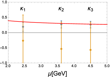
In this figure, we compare with its naively expected value, , while taking the renormalization scale as . Note that is multiplied since the LO result in the continuum theory is . In plotting the running coupling, we assume and . The determined ’s are consistent with the naively expected values within the statistical errors, which supports validity of our analysis. Large statistical errors for stem from the small number of data for .
We show the lattice result in the continuum limit [Eq. (40)] and the OPE prediction [Eq. (41)] which are determined by the fit in Fig. 11. From the figure, one can see that the analysis is performed reasonably, and that the OPE calculation and the lattice result are mutually consistent in the examined region.

For convenience, we summarize the conditions used in our main analysis, with which we determine the central value of .
- •
Controlling finite effects: The data at are used combined with the tree-level correction.
- •
Singlet potential: defined by Eq. (11), which has accuracy
- •
Regularization of US divergence: Prescription I [Eq. (21)]
- •
Quark masses: We use the lattice data obtained with unphysical quark mass inputs and in the massless quark approximation.
- •
Matching range:
Now we estimate systematic errors of our determination. We perform the following re-analyses. Since this analysis will give our final result, some additional aspects are studied in comparison to Analysis (I).
- •
Finite effects: We use the lattice data at . In this case, we omit the tree-level correction by setting ’s to zero. This is because the role of the tree-level correction is similar to that of the -term under the current hierarchy , where the tree-level correction is well approximated in expansion in .2727 27 If we include both ’s and ’s, the fit is destabilized due to a flat direction caused by this degeneracy. We adopt the -term rather than the tree-level correction since the tree-level correction becomes less reliable when the matching range shifts to lower energy region.
- •
Higher order uncertainty: We replace in matching as
(44) with or in order to estimate higher order uncertainty; see Eq. (24) for .
- •
US regularization: We adopt the regularization method II, given by Eq. (22). We have chosen as and .
- •
Mass effects: Lattice data are obtained with the unphysical mass inputs. We include an estimation of this mass difference effect as a systematic error, since we do not know the true correction. We estimate the lattice data on the physical point as
(45) where is the masses for the light quarks (); is the finite mass correction evaluated in perturbative QCD at [41, 42, 43]. More precisely, it is a function of of the form
(46) which vanishes in the limit . In the above estimation, we take the renormalization scale as and choose as 0.27, 0.23, 0.21 for , respectively, so that it is close to . For the mass values of the light quarks, we use . To model a nonperturbative effect, we also substitute a constituent quark mass of for in Eq. (45) as an additional test (while the other parameters are kept fixed). Furthermore, since is obtained by treating the light quarks as massless, the finite mass effects are also added to as
(47) For this , we take and . In this way, we estimate both theoretical prediction and lattice result at the physical point.
- •
Matching range: We vary the range of the lattice result used in the matching as
(48) to examine the stability of the OPE truncated at .
- •
Factorization scheme: In extracting the renormalon free part , we rewrite the integrand of by a complex function; see (56) in Appendix B. In general, there can be other choices for this function, and in this regard, we have chosen a certain scheme. A different scheme practically causes an difference in the OPE prediction truncated at ; see Ref. [16] for details.2828 28 In Ref. [16], it is shown that the current choice is natural from the viewpoint of analyticity. To see an effect of this scheme dependence, we add an -term in the fit so that this scheme dependence is absorbed. (Note that, in order to determine coefficients up to higher orders in , a wider fitting range is required. We choose the range in this analysis as , where and are stable against variation of the range.2929 29 This range is chosen after studying the stability for various ranges.)
- •
Lattice spacing: The lattice spacing , used to convert and into physical units, has an error as shown in table 1, and has an additional error of 1.7 % due to the uncertainty of the physical value of the Wilson-flow scale [44]. For the former one, the error is etimated by the largest deviation detected from a set of six data, , where denotes the error shown in table 1. The error associated with the latter is estimated by shifting all the ’s simultaneously by its uncertainty. By combining these two errors in in quadrature, the uncertainty from the lattice spacing is estimated.
The estimated systematic errors are summarized in table 7. Some error sources included in Analysis (I) are absent thanks to the first-principle nature of this analysis.
| finite | h.o. | US | Mass | range | fact. scheme | latt. spacing | |
|---|---|---|---|---|---|---|---|
| Obtained value | |||||||
| Assigned error |
In addition, most of the systematic errors are reduced compared to Analysis (I). In particular, the higher order uncertainty is smaller since a shorter distance region is used; see Fig. 2. The mass effects turn out to be negligibly small even if we consider the constituent quark mass. This is because we are probing a sufficiently short-distance region. (Additional analyses on systematic errors are given in Appendix F.)
As a result of Analysis (II), we obtain
| (49) |
3.4 Summary of results
We have performed two determinations of . In Analysis (I), which is a preparatory analysis, we first took the continuum limit of the lattice data, and then we matched the result with the OPE prediction. Although this analysis partially relies on a model-like assumption, we explicitly showed that (a) the continuum extrapolation of the lattice data can be taken smoothly, and that (b) the OPE combined with our renormalon subtraction is indeed consistent; see Fig. 8. We obtained and . The total errors are obtained by combining the statistic and systematic errors in quadrature.
In Analysis (II), we performed a global fit, where theoretical constraints are fully used. Analysis (II) is superior to Analysis (I) in the sense that it is a first-principle analysis and that our dominant error, higher order uncertainty, is reduced thanks to the use of short distance range. This gives our final result:
| (50) |
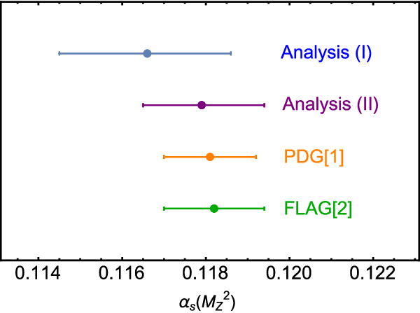
One can see that both analyses give consistent values. Our results of are compared with the current PDG and FLAG results in Fig. 12, where one can see that our results are also consistent with them.
4 Conclusions and discussion
We determined the strong coupling constant from the static QCD potential by matching a lattice result with a new OPE calculation where renormalons are subtracted from the leading Wilson coefficient. We subtract both and renormalons from the Wilson coefficient. In particular, we confirmed the following features regarding the renormalon subtraction.
- 1.
Theoretically the cancellation of the renormalon against the nonperturbative term is checked at the LL order. Furthermore, logarithmic contributions at IR region in the Fourier integral, which cause factorial divergence, are subtracted at the NNNLL level.
- 2.
To check that ignoring renormalons contained in is harmless at the current level of the analysis, we confirmed that the renormalon-free Wilson coefficient approaches the lattice data as we raise the order: LL, NLL, NNLL, NNNLL (Fig. 7).
- 3.
As a result of the renormalon subtraction, convergence and stability against scale variation are improved as compared to the conventional methods. The difference between the Wilson coefficient and the lattice data can be fitted with consistently with the prediction of the OPE. This behavior is observed up to ( fm). (Figs. 8,9)
Based on these confirmations, we adopt the OPE framework where a power correction term of order is added to the renormalon-free Wilson coefficient.
In our determination, the matching range is taken as based on the above observation. This range is significantly wider than preceding determinations using the static QCD potential, where typically has been used. This enables us to use the data not only at but also at , where lattice simulation is considered to be accurate. We performed a reasonable fit in this wide region, which leads to a reliable determination. Our final result is . This result is obtained by a global fit [Analysis (II)] and is consistent with our another analysis [Analysis (I)], where we examined intermediate processes step by step. The reasonable value of with respect to today’s other determinations again indicates the validity of our analysis. We also confirmed that although the energy region extends to lower energy side than conventional determinations using perturbative calculation, varying the matching range does not induce significant systematic errors.
Dominant error of our determination comes from systematic errors, in particular from the higher order perturbative uncertainty of the leading Wilson coefficient. We emphasize that a finer lattice simulation will straightforwardly reduce this error, since we can adopt a shorter distance range in the fit, where the uncertainty becomes smaller.3030 30 Reduction of the higher order uncertainty can be estimated as follows. The relative perturbative accuracy in our formulation at LL is order , not affected by renormalon uncertainties. Here, is the typical scale used in the determination. For instance, suppose that currently , and suppose that can be raised by a factor 2 (corresponding to twice finer lattices). Then the perturbative error would reduce, which is multiplied by –0.4. ,3131 31 We remark that if the coarsest lattice becomes finer while the finest lattice spacing is kept fixed, it serves to reduce the error. This is because our current range is chosen so that the number of data points from the coarsest lattice is sufficient.
We believe that our analyses are useful not only in determining but also in promoting understanding on the OPE structure and lattice discretization errors. As stated, this is a first numerical observation that the difference between the Wilson coefficient and the lattice result is consistent with behavior at in accordance with the OPE structure. We also give a constraint on the linear term in in the difference, which should be zero in the OPE. (See discussion in Sec. 3.2.2.) Concerning the lattice discretization error, we clarified that (i) the data at indeed has a serious finite effect (Appendix E), and (ii) once the tree-level correction is considered combined with the OPE calculation, the finite effect can be largely removed with reasonable values of lattice effective couplings.
Acknowledgements The authors are grateful to the JLQCD collaboration for providing the lattice data. They thank G. Mishima for collaboration at an early stage of this study and also thank S. Aoki, S. Hashimoto, T. Onogi, and S. Sasaki for fruitful discussion. The works of Y.K. and Y.S. are supported in part by Grant-in-Aid for scientific research (Nos. 26400255 and 17K05404) from MEXT, Japan.
Appendix A Coefficients of perturbative calculation
Appendix B Formulation to extract from
We explain the formula to extract from Eq. (7). We reduce Eq. (7) to the one-dimensional integral representation:
| (55) |
with . We rewrite the integral as
| (56) |
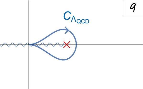
The contours and are displayed in Fig. 13.


The integral along is clearly independent of . Although the integral along looks dependent, it contains a -independent part. We evaluate this integral as
| (57) |
since . In expansion of the exponential factor, the real and pure imaginary coefficients appear in turn.
The terms with real coefficients satisfy the relation . Owing to this, these parts can be calculated as
| (58) |
with
| (59) |
| (60) |
where is shown in Fig. 14.
The coefficients and are independent and real. Numerical evaluation of these coefficients is sufficient for our purpose. [ is given by Eq. (12).] We remark that the analytical results up to LL can be found in Ref. [15].
On the other hand, the terms with imaginary coefficients do not satisfy the relation , and the above deformation cannot be applied. Therefore, we have
| (61) |
where dependence remains.
Based on the above argument, we can construct a -independent quantity . Note that a -independent part is also given by the integral along . Then by collecting all the -independent part, we obtain
| (62) |
with
| (63) |
In the last line, we rotate the contour to the line along with real positive .
Once the -dependent part of is considered as well, one obtains the decomposition shown in Eq. (10).
Appendix C Definition of
The definition of the scale in the scheme, , is given by
| (64) |
where represents the coupling at the renormalization scale . We approximate the function at four-loop as in Eq. (9), which gives the definition of , used extensively in this paper.
Appendix D and covariance matrix
We present definitions of and covariance matrices used in our analyses, which may be useful especially for non-expert readers.
Interpolation [Analysis (I)] We define in the interpolation with a covariance matrix as3232 32 is a dimensionless quantity. Accordingly, each quantity appearing in Eq. (65) can be made dimensionless. In practice, we normalize all the quantities with .
| (65) |
where is defined in Eq. (26) and run over the lattice points under consideration. The covariance matrix is calculated as
| (66) |
in the jackknife method, where is the number of bins for the -th lattice simulation; see table 1. If the subscript is shown, it expresses a covariance matrix among the potentials .3333 33 Although in Analysis (I) we treat the data separately according to each direction, we will use them simultaneously in Analysis (II). This is the reason why we suppress the subscript in Eq. (66).
Continuum extrapolation [Analysis (I)] in the extrapolation to the continuum limit is defined as
| (67) |
where is defined by Eq. (27).
The covariance matrix for is calculated as
| (68) |
Note that in the continuum extrapolation, the jackknife samples with the size are generated since we have three independent lattice measurements. We present the numerical result of in table 8.
| 0.7196 | 0.7822 | 1.043 | 1.079 | 1.304 | 1.439 | |
|---|---|---|---|---|---|---|
| 0.7196 | ||||||
| 0.7822 | ||||||
| 1.043 | ||||||
| 1.079 | ||||||
| 1.304 | ||||||
| 1.439 |
Matching [Analysis (I)] We define in the matching of Analysis (I) as
| (69) |
where is given in Eq. (30) and is the covariance matrix for :
| (70) |
Global fit [Analysis (II)] We define in the global fit in Analysis (II) as
| (71) |
Here, the covariance matrix consists of three matrices of dimension and in a block diagonal form:
| (72) |
where the definition of each matrix is given by Eq. (66).
Appendix E Case including data at in Analysis (I)
In Analysis (I), we do not use the data at in interpolating lattice data in our analyses, in order to suppress serious finite effects. Here, let us see what happens if we include this shortest point.


We interpolate lattice data including the ones at , and obtain in the same way. In Fig. 15, we plot the data points of taking the horizontal axis as . One can see that they do not obey linear behaviors in . We remark that even the data for , where the finite effect is considered to be well suppressed, cannot smoothly be extrapolated to the continuum limit. It shows that the data at , which has a small statistical error, dominantly contributes to determining the interpolating function, and thus, the interpolating function is seriously distorted. In Fig. 16, we show in this case, corresponding to Fig. 5.


Extrapolations to the continuum limit do not work for . For , where the shortest point is located at , extrapolations work better than for . We conclude that the data at has serious discretization error, and we should be cautious about treating it.
Appendix F Additional analyses on systematic errors
In this appendix, we provide supplemental analyses to check validity of our error analyses from additional aspects.
effect
In Sec. 3, we considered the leading discretization error, the quadratic effect in , of the lattice data.
Here, we estimate the possible effect coming from the neglected error.3434
34
Due to chiral symmetry, an error is prohibited.
In both Analyses (I) and (II), if we perform fits including terms it turns out that the fits have little sensitivities to these terms, given the current lattice data. As a result, the fits become fairly unstable, leading to fairly uncertain results for [even though they are consistent with Eqs. (32) and (43) within estimated (large) errors].
Instead we can confirm that our analysis is stable against possible effects in
the following way in the case of Analysis (II).
We add an -term to Eq. (40) as while fixing .
In this analysis, to properly consider the expansion in up to NLO,
we omit the data at because
this expansion is not legitimate when the data at is included, as clarified in Appendix E.
In this case, the tree-level correction is not necessary and is omitted (see footnote 27).
To assume a reasonable size of , we refer to the size of ,
the coefficients of the error,
determined from the data at . They read .
Then, we assume and vary to .
The other parameters (such as and ) are treated as fitting parameters.
The largest variation of caused by the -term is obtained as
.
This is comparable to the assigned error in Table 7 in Analysis (II).
This result indicates that our error analysis concerning finite effects is reasonable
even if we take into account the neglected higher order discretization errors.
Mass correction
In Sec. 3.3, the effect of the mass deviation in the lattice simulations was estimated based on perturbation theory,
where it was found negligibly small.
We support this result by directly comparing lattice results with different pion masses.
We analyze the lattice data with and for the lattice spacing [25].
(Here, we neglect finite effects.)
Since the slope of the potential affects ,
we examine the difference of the slopes.
The slopes are approximately obtained from the difference of the potentials at the nearest neighbor.
In Fig. 17, the difference of the (approximate) slopes is shown,
where it is consistent with zero.3535
35
The slope itself (before taking the difference) is about 0.1 in the same units.
(In Analysis (II), we use the first 10 points.)
This result is consistent with our error estimate that the mass effect is negligibly small.

Possible logarithmic correction to -term
We have treated the nonperturbative effect as .
There is a possibility that this -term is modified by logarithmic corrections,
which may stem from higher order computations of Wilson coefficients.
Here, we examine how large such a logarithmic correction affects our determination.
In Analysis (II), we assume as
| (73) |
with . Then, we obtain the result in Table 9. (We also use 1.5 GeV and 0.5 GeV instead of 1 GeV as a scale in the logarithm. We find that the results hardly change.)
| 0.1 | 0.3 | |||
|---|---|---|---|---|
| [GeV3] | ||||
| 2 | 1 | 0 |
One sees that this uncertainty dose not induce a dominant systematic error, and thus, is not included in our final result.
References
- (1) C. Patrignani, et al., [Particle Data Group], “Review of particle physics,” Chinese Physics C 40 no. 10, (10, 2016) .
- (2) S. Aoki et al., “Review of lattice results concerning low-energy particle physics,” Eur. Phys. J. C77 no. 2, (2017) 112, arXiv:1607.00299 [hep-lat].
- (3) K. Maltman, D. Leinweber, P. Moran, and A. Sternbeck, “The Realistic Lattice Determination of alpha(s)(M(Z)) Revisited,” Phys. Rev. D78 (2008) 114504, arXiv:0807.2020 [hep-lat].
- (4) S. Aoki et al., (PACS-CS Collaboration), “Precise determination of the strong coupling constant in N(f) = 2+1 lattice QCD with the Schrodinger functional scheme,” JHEP 10 (2009) 053, arXiv:0906.3906 [hep-lat].
- (5) C. McNeile, C. T. H. Davies, E. Follana, K. Hornbostel, and G. P. Lepage, “High-Precision c and b Masses, and QCD Coupling from Current-Current Correlators in Lattice and Continuum QCD,” Phys. Rev. D82 (2010) 034512, arXiv:1004.4285 [hep-lat].
- (6) B. Chakraborty, C. T. H. Davies, B. Galloway, P. Knecht, J. Koponen, G. C. Donald, R. J. Dowdall, G. P. Lepage, and C. McNeile, “High-precision quark masses and QCD coupling from lattice QCD,” Phys. Rev. D91 no. 5, (2015) 054508, arXiv:1408.4169 [hep-lat].
- (7) A. Bazavov, N. Brambilla, X. Garcia i Tormo, P. Petreczky, J. Soto, and A. Vairo, “Determination of from the QCD static energy: An update,” Phys. Rev. D90 no. 7, (2014) 074038, arXiv:1407.8437 [hep-ph].
- (8) M. Luscher, P. Weisz, and U. Wolff, “A Numerical method to compute the running coupling in asymptotically free theories,” Nucl. Phys. B359 (1991) 221–243.
- (9) M. Luscher, R. Narayanan, P. Weisz, and U. Wolff, “The Schrodinger functional: A Renormalizable probe for nonAbelian gauge theories,” Nucl. Phys. B384 (1992) 168–228, arXiv:hep-lat/9207009 [hep-lat].
- (10) M. Luscher, R. Sommer, P. Weisz, and U. Wolff, “A Precise determination of the running coupling in the SU(3) Yang-Mills theory,” Nucl. Phys. B413 (1994) 481–502, arXiv:hep-lat/9309005 [hep-lat].
- (11) S. Sint, “On the Schrodinger functional in QCD,” Nucl. Phys. B421 (1994) 135–158, arXiv:hep-lat/9312079 [hep-lat].
- (12) M. Bruno, M. Dalla Brida, P. Fritzsch, T. Korzec, A. Ramos, S. Schaefer, H. Simma, S. Sint, and R. Sommer, (ALPHA Collaboration),“QCD Coupling from a Nonperturbative Determination of the Three-Flavor Parameter,” Phys. Rev. Lett. 119 no. 10, (2017) 102001, arXiv:1706.03821 [hep-lat].
- (13) M. Beneke, “Renormalons,” Phys. Rept. 317 (1999) 1–142, arXiv:hep-ph/9807443 [hep-ph].
- (14) A. H. Mueller, “On the Structure of Infrared Renormalons in Physical Processes at High-Energies,” Nucl. Phys. B250 (1985) 327–350.
- (15) Y. Sumino, “Static QCD Potential at : Perturbative Expansion and Operator-Product Expansion,” Phys. Rev. D76 (2007) 114009, arXiv:hep-ph/0505034 [hep-ph].
- (16) G. Mishima, Y. Sumino, and H. Takaura, “Subtracting infrared renormalons from Wilson coefficients: Uniqueness and power dependences on QCD,” Phys. Rev. D95 no. 11, (2017) 114016, arXiv:1612.08711 [hep-ph].
- (17) M. Beneke, “A Quark Mass Definition Adequate for Threshold Problems,” Phys. Lett. B434 (1998) 115–125, arXiv:hep-ph/9804241 [hep-ph].
- (18) A. H. Hoang, M. C. Smith, T. Stelzer, and S. Willenbrock, “Quarkonia and the pole mass,” Phys. Rev. D59 (1999) 114014, arXiv:hep-ph/9804227 [hep-ph].
- (19) N. Brambilla, A. Pineda, J. Soto, and A. Vairo, “Potential NRQCD: an Effective Theory for Heavy Quarkonium,” Nucl. Phys. B566 (2000) 275, arXiv:hep-ph/9907240 [hep-ph].
- (20) A. V. Smirnov, V. A. Smirnov, and M. Steinhauser, “Fermionic contributions to the three-loop static potential,” Phys. Lett. B668 (2008) 293–298, arXiv:0809.1927 [hep-ph].
- (21) C. Anzai, Y. Kiyo, and Y. Sumino, “Static QCD Potential at Three-Loop Order,” Phys. Rev. Lett. 104 (2010) 112003, arXiv:0911.4335 [hep-ph].
- (22) A. V. Smirnov, V. A. Smirnov, and M. Steinhauser, “Three-Loop Static Potential,” Phys. Rev. Lett. 104 (2010) 112002, arXiv:0911.4742 [hep-ph].
- (23) R. N. Lee, A. V. Smirnov, V. A. Smirnov, and M. Steinhauser, “Analytic Three-Loop Static Potential,” Phys. Rev. D94 no. 5, (2016) 054029, arXiv:1608.02603 [hep-ph].
- (24) T. Kaneko, S. Aoki, G. Cossu, H. Fukaya, S. Hashimoto, and J. Noaki, (JLQCD Collaboration),“Large-scale simulations with chiral symmetry,” PoS LATTICE2013 (2014) 125, arXiv:1311.6941 [hep-lat].
- (25) JLQCD Collaboration, in preparation
- (26) F. Karbstein, M. Wagner, and M. Weber, “Determination of and analytic parameterization of the static quark-antiquark potential,” arXiv:1804.10909 [hep-ph].
- (27) H. Takaura, T. Kaneko, Y. Kiyo, and Y. Sumino, “Determination of from static QCD potential with renormalon subtraction,” Phys. Lett. B789 (2019) 598–602, arXiv:1808.01632 [hep-ph].
- (28) H. Takaura, “Renormalon free part of an ultrasoft correction to the static QCD potential,” Phys. Lett. B783 (2018) 350–356, arXiv:1712.05435 [hep-ph].
- (29) T. Appelquist, M. Dine, and I. J. Muzinich, “The Static Potential in Quantum Chromodynamics,” Phys. Lett. 69B (1977) 231–236.
- (30) N. Brambilla, A. Pineda, J. Soto, and A. Vairo, “The Infrared behavior of the static potential in perturbative QCD,” Phys. Rev. D60 (1999) 091502, arXiv:hep-ph/9903355 [hep-ph].
- (31) P. Weisz, “Continuum Limit Improved Lattice Action for Pure Yang-Mills Theory. 1.,” Nucl. Phys. B212 (1983) 1–17.
- (32) R. C. Brower, H. Neff, and K. Orginos Comput. Phys. Commun. 220 (2017) 1–19, arXiv:1206.5214 [hep-lat].
- (33) “Properties and uses of the Wilson flow in lattice QCD,” JHEP 08 (2010) 071, arXiv:1006.4518 [hep-lat]. [Erratum: JHEP03,092(2014)].
- (34) M. Tomii, G. Cossu, B. Fahy, H. Fukaya, S. Hashimoto, T. Kaneko, and J. Noaki, (JLQCD Collaboration), “Renormalization of domain-wall bilinear operators with short-distance current correlators,” Phys. Rev. D94 no. 5, (2016) 054504, arXiv:1604.08702 [hep-lat].
- (35) G. S. Bali and K. Schilling, “Static quark - anti-quark potential: Scaling behavior and finite size effects in SU(3) lattice gauge theory,” Phys. Rev. D46 (1992) 2636–2646.
- (36) A. Bazavov et al., (MILC Collaboration),“Results for light pseudoscalar mesons,” PoS LATTICE2010 (2010) 074, arXiv:1012.0868 [hep-lat].
- (37) A. Bazavov et al., “The chiral and deconfinement aspects of the QCD transition,” Phys. Rev. D85 (2012) 054503, arXiv:1111.1710 [hep-lat].
- (38) R. Sommer, “Scale setting in lattice QCD,” PoS LATTICE2013 (2014) 015, arXiv:1401.3270 [hep-lat].
- (39) Y. Sumino, Lecture Note, “Understanding Interquark Force and Quark Masses in Perturbative QCD,” 2014. arXiv:1411.7853 [hep-ph]. http://inspirehep.net/record/1331450/files/arXiv:1411.7853.pdf.
- (40) K. G. Chetyrkin, B. A. Kniehl, and M. Steinhauser, “Strong coupling constant with flavor thresholds at four loops in the MS scheme,” Phys. Rev. Lett. 79 (1997) 2184–2187, arXiv:hep-ph/9706430 [hep-ph].
- (41) A. H. Hoang, “Bottom quark mass from Upsilon mesons: Charm mass effects,” arXiv:hep-ph/0008102 [hep-ph].
- (42) M. Melles, “The Static QCD potential in coordinate space with quark masses through two loops,” Phys. Rev. D62 (2000) 074019, arXiv:hep-ph/0001295 [hep-ph].
- (43) S. Recksiegel and Y. Sumino, “Perturbative QCD potential, renormalon cancellation and phenomenological potentials,” Phys. Rev. D65 (2002) 054018, arXiv:hep-ph/0109122 [hep-ph].
- (44) S. Borsanyi et al., “High-precision scale setting in lattice QCD,” JHEP 09 (2012) 010, arXiv:1203.4469 [hep-lat].