跳到论文正文
W Papers独立论文阅读器 arXiv:1808.01236 论文正文 计算阅读时间 · 0%
引用这篇论文根据当前论文元数据生成,正式投稿前建议核对。


License: arXiv.org perpetual non-exclusive license
arXiv:1808.01236v1 [stat.ME] 03 Aug 2018

Bayesian Change Point Detection for Functional Data

Operations Research Graduate Program, North Carolina State University, xli35@ncsu.eduDepartment of Statistics, North Carolina State University, sghosal@stat.ncsu.edu
Xiuqi Li    Subhashis Ghosal
Abstract

We propose a Bayesian method to detect change points for functional data. We extract the features of a sequence of functional data by the discrete wavelet transform (DWT), and treat each sequence of feature independently. We believe there is potentially a change in each feature at possibly different time points. The functional data evolves through such changes throughout the sequences of observations. The change point for this sequence of functional data is the cumulative effect of changes in all features. We assign the features with priors which incorporate the characteristic of the wavelet coefficients. Then we compute the posterior distribution of change point for each sequence of feature, and define a matrix where each entry is a measure of similarity between two functional data in this sequence. We compute the ratio of the mean similarity between groups and within groups for all possible partitions, and the change point is where the ratio reaches the minimum. We demonstrate this method using a dataset on climate change.
Keywords: Change point detection, Functional data, Discrete wavelet transform, Posterior consistency

and

1 Introduction

Change point detection has always been an important aspect in data analysis. In recent years, there are increasing interests in developing methods to detect change point for functional data. Berkes et al. (2009) developed a method that works with the difference of mean functions projected on the principal components of the data. Zhang et al. (2011) developed a self-normalization (SN) based test to identify potential change points in the dependence structure of functional observations. Aston and Kirch (2012) also proposed a method to detect change points for dependent functional observations, and they were particularly interested in the case where the change point is an epidemic change (a change occurs and then the observations return to baseline at a later time). Sharipov et al. (2016) developed a new test for structural changes in functional data that based on Hilbert space theory and critical values are deduced from bootstrap iterations. Aue et al. (2018) proposed a method to uncover structural breaks in functional data that does not rely on dimension reduction techniques.

In this paper, we propose a Bayesian method to detect change points for functional data. We extract the features of a sequence of functional data by the discrete wavelet transform (DWT), and treat each sequence of feature independently. We believe there is potentially a change in each feature at possibly different time points. The functional data evolves through such changes throughout the sequence of observations. The change point for this sequence of functional data is the cumulative effect of changes in all features. Such gradual evolutionary model for changes seems to be very appropriate for functional data, since functions have many aspects and it is hard to imagine that all those change at once. When such a cumulative effect becomes substantial to make the following functional observations significantly dissimilar with the previous ones—in that the variation across the two groups relative to the variation within the two groups is the maximum at that time point. We assign the features with priors which incorporate the characteristic of the wavelet coefficients. Then we compute the posterior distribution of change point for each sequence of feature, and define a matrix where each entry is a measure of similarity between two functional data in this sequence. We compute the ratio of the mean similarities between groups and within groups for all possible partitions, and the change point is where the ratio reaches the minimum. Once we have detected one change point, we can successively apply the procedure to subgroups divided by the change point. We can continue finding the change points in subgroups until a stopping criterion has been met. For example, we can stop if a certain number of change points have been detected, or there is no significant difference in the previous and following observations. Thus, this method can be inherently extended to multiple change points detection.

2 Model

We follow the formulation of Suarez and Ghosal (2016) for the structure of functional observations, who applied their model in the context of clustering. We extend their approach to change point detection for functional data, which can be regarded as a special case of clustering with the constraint that for each characteristic, there are at most two clusters and they are linearly ordered. Suppose that the functional observations arise from true signals fi​(t)f_{i}(t), t∈[0,1]t\in[0,1], i=1,…,ni=1,\dots,n, corrupted by some noise process, where nn denotes the sample size. We observe the functional data at some discrete time points. Then the model can be represented as

Yi​(Tl)=fi​(Tl)+εi​l,\displaystyle Y_{i}(T_{l})=f_{i}(T_{l})+\varepsilon_{il}, (1)

where εi​l\varepsilon_{il} is assumed to follow a normal distribution with mean 0 and variance σ2\sigma^{2}, and is independent across ii and ll. Let Yi=(Yi​(T1),…,Yi​(Tm))TY_{i}=(Y_{i}(T_{1}),\dots,Y_{i}(T_{m}))^{T} be the iith obsvervation at points T1,…,TmT_{1},\dots,T_{m}, where Tl∈[0,1]T_{l}\in[0,1], for l=1,…,ml=1,\dots,m. Similarly, let fi=(fi​(T1),…,fi​(Tm))Tf_{i}=(f_{i}(T_{1}),\dots,f_{i}(T_{m}))^{T}, and εi=(εi​(T1),…,εi​(Tm))T\varepsilon_{i}=(\varepsilon_{i}(T_{1}),\dots,\varepsilon_{i}(T_{m}))^{T}. For functional data, the discrete wavelet transform (DWT) is one of the most common feature extraction technique. To implement the DWT, mm needs to be a power of 2, and T1,…,TmT_{1},\dots,T_{m} need to be equidistant. For mm that is not a power of 2, we can first smooth to obtain a function, and then take a power of 2 number of discrete points from that function. In terms of the orthonormal basis {ϕ0}∪{ψj​k:j=0,…,J−1,k=0,…,2j−1}\{\phi_{0}\}\cup\{\psi_{jk}:j=0,\dots,J-1,k=0,\dots,2^{j}-1\}, we can define the following DWT operator (Antoniadis et al., 2013):

W:ℝm→ℝm,f→(α0,β0,…,βJ−1),\displaystyle W:\mathbb{R}^{m}\rightarrow\mathbb{R}^{m},\>\>f\rightarrow(\alpha_{0},\beta_{0},\dots,\beta_{J-1}), (2)

with βj=(βj,0,…,βj,2j−1)\beta_{j}=(\beta_{j,0},\dots,\beta_{j,2^{j}-1}). Applying the DWT operator on Yi=fi+εiY_{i}=f_{i}+\varepsilon_{i}, then we have

W​Yi=W​fi+W​εi,\displaystyle WY_{i}=Wf_{i}+W\varepsilon_{i}, (3)

where W​εi=dεiW\varepsilon_{i}\stackrel{{\scriptstyle d}}{{=}}\varepsilon_{i} by the orthogonality of WW. Let α0\alpha_{0} denote the scaling coefficient at the level 0, and βj​k\beta_{jk} be the wavelet coefficients at the multiresolution level j,kj,k. As a result, (3) can be rewritten as

a0(i)=α0(i)+e0(i),bj​k(i)=βj​k(i)+ej​k(i),\displaystyle a^{(i)}_{0}=\alpha^{(i)}_{0}+e^{(i)}_{0},\>\>b^{(i)}_{jk}=\beta^{(i)}_{jk}+e^{(i)}_{jk}, (4)

where e0(i)e_{0}^{(i)} and ej​k(i)e_{jk}^{(i)} follow a normal distribution with mean 0 and variance σ2\sigma^{2}, for k=0,…,2j−1,j=0,…,J−1k=0,\dots,2^{j}-1,j=0,\dots,J-1.

When the functional data are (essentially) observed continuously in time, we also consider the following infinite Gaussian white noise model

d​Yi​(t)=fi​(t)​d​t+σ​d​Bi​(t),\displaystyle dY_{i}(t)=f_{i}(t)dt+\sigma dB_{i}(t), (5)

where Bi​(⋅)B_{i}(\cdot) are independent Brownian motions on [0,1][0,1]. Let

a0(i)=∫01ϕ0(t)dYi(t),α0(i)=∫01ϕ0(t)fi(t)dt,bj​k(i)=∫01ψj​k(t)dYi(t),βj​k(i)=∫01ψj​k(t)fi(t)dt,e0(i)=σ∫01ϕ0(t)dBi(t),ej​k(i)=σ∫01ψj​k(t)dBi(t).\displaystyle\begin{split}&a_{0}^{(i)}=\int_{0}^{1}\phi_{0}(t)dY_{i}(t),\>\alpha_{0}^{(i)}=\int_{0}^{1}\phi_{0}(t)f_{i}(t)dt,\\ &b_{jk}^{(i)}=\int_{0}^{1}\psi_{jk}(t)dY_{i}(t),\>\beta_{jk}^{(i)}=\int_{0}^{1}\psi_{jk}(t)f_{i}(t)dt,\\ &e_{0}^{(i)}=\sigma\int_{0}^{1}\phi_{0}(t)dB_{i}(t),\>e_{jk}^{(i)}=\sigma\int_{0}^{1}\psi_{jk}(t)dB_{i}(t).\end{split} (6)

Then e0(i)e_{0}^{(i)} and ej​k(i)e_{jk}^{(i)} follow the normal distribution with mean 0 and variance σ2\sigma^{2}, for k=0,…,2j−1k=0,\dots,2^{j}-1, j=1,2,…j=1,2,\dots, independent of each other, for each i=1,…,ni=1,\dots,n.

To detect the change point of this sequence of functional data, we first find the change in each component, that is, we detect the change for each feature βj​k\beta_{jk}, and we decide the overall change point from them.

In the section on posterior consistency, we state the results only in terms of the infinite model. However, in practice, we can only work with the finite model. By letting βj​k(i)=0\beta_{jk}^{(i)}=0 for all j>Jj>J, the infinite model can be related to the finite one with a random JJ. If the coefficients are obtained following the schema of Abramovich et al. (1998), then JJ will have a limiting Poisson distribution by Proposition 1 of Suarez and Ghosal (2016). Under this schema, the total number of nonzero coefficients also has a limiting Poisson distribution.

3 Prior Distributions

For each βj​k(i)\beta^{(i)}_{jk}, we define the following probabilities:

P(β(i)j​k≠0)=πj,P(β(i)j​k=0)=1−πj.\displaystyle\begin{split}&\text{P}(\beta^{(i)}_{jk}\neq 0)=\pi_{j},\ \text{P}(\beta^{(i)}_{jk}=0)=1-\pi_{j}.\end{split} (7)

As the wavelet coefficients of a signal function are sparse, Abramovich et al. (1998) proposed the following priors incorporating this characteristic feature of wavelet coefficients:

βj​k(i)∼indπj​N​(0,cj2​σ2)+(1−πj)​δ0,\displaystyle\begin{split}\beta^{(i)}_{jk}\stackrel{{\scriptstyle\text{ind}}}{{\sim}}\pi_{j}\text{N}(0,c^{2}_{j}\sigma^{2})+(1-\pi_{j})\delta_{0},\end{split} (8)

where δ0\delta_{0} is a point mass at 0, and the hyperparameters in (8) are given by

cj2=ν12−γ1​j,πj=min(1,ν22−γ2​j),j=0,…,J−1,\displaystyle c_{j}^{2}=\nu_{1}2^{-\gamma_{1}j},\>\pi_{j}=\text{min}(1,\nu_{2}2^{-\gamma_{2}j}),\>j=0,\dots,J-1, (9)

and ν1,ν2,γ1≥0\nu_{1},\nu_{2},\gamma_{1}\geq 0, and 0≤γ2≤10\leq\gamma_{2}\leq 1. A vague prior is placed on α0\alpha_{0}.

Let ψ\psi be a mother wavelet function of regularity rr. Consider constants ss, pp and qq such that max​(0,1/p−1/2)<s<r\text{max}(0,1/p-1/2)<s<r, 1≤p,q≤∞1\leq p,q\leq\infty. If either

s+12−γ2p−γ12<0,\displaystyle\begin{split}&s+\frac{1}{2}-\frac{\gamma_{2}}{p}-\frac{\gamma_{1}}{2}<0,\end{split} (10)

or

s+12−γ2p−γ12=0,and 0≤γ2<1,1≤p<∞,q=∞,\displaystyle\begin{split}&s+\frac{1}{2}-\frac{\gamma_{2}}{p}-\frac{\gamma_{1}}{2}=0,\>\text{and}\>0\leq\gamma_{2}<1,1\leq p<\infty,q=\infty,\end{split} (11)

then f∈ℬp,qsf\in\mathcal{B}^{s}_{p,q} almost surely, where ℬp,qs\mathcal{B}^{s}_{p,q} denotes Besov space of index (p,q)(p,q) and smoothness ss (Abramovich et al., 1998).

The prior on σ\sigma is given by

σ2∼IG​(θ,λ),\displaystyle\sigma^{2}\sim\text{IG}(\theta,\lambda), (12)

where IG stands for the inverse gamma distribution. Let gg denote the density funciton of the inverse-gamma distribution.

4 Posterior Probabilities of Change Point

For any j,kj,k, let τj​k\tau_{jk} denote the change point, and let τj​k\tau_{jk} take possible values 1,…,n1,\dots,n. Let ρi\rho_{i} denote the prior probability of changing at point ii, where ρi>0\rho_{i}>0, ∑i=1nρi=1\sum^{n}_{i=1}\rho_{i}=1, and i=1,…,ni=1,\dots,n. Then the posterior probability of τj​k=i\tau_{jk}=i is

P​(τj​k=i|bj​k(1),…,bj​k(n))=P​(bj​k(1),…,bj​k(n)|τj​k=i)​ρi∑l=1NP​(bj​k(1),…,bj​k(n)|τj​k=l)​ρl.\displaystyle\text{P}(\tau_{jk}=i|b^{(1)}_{jk},\dots,b^{(n)}_{jk})=\frac{\text{P}(b^{(1)}_{jk},\dots,b^{(n)}_{jk}|\tau_{jk}=i)\rho_{i}}{\sum^{N}_{l=1}\text{P}(b^{(1)}_{jk},\dots,b^{(n)}_{jk}|\tau_{jk}=l)\rho_{l}}. (13)

The main problem is to compute the marginal likelihood P​(bj​k(1),…,bj​k(n)|τj​k=i)\text{P}(b^{(1)}_{jk},\dots,b^{(n)}_{jk}|\tau_{jk}=i). When τj​k=1\tau_{jk}=1, it is the initial state meaning no change. For τj​k=2,…,n\tau_{jk}=2,\dots,n, the marginal likelihood is derived from four scenarios: change from zero to zero (which is no change), change from zero to non-zero, change from non-zero to zero, and change from non-zero to non-zero.

4.1 Initial State

When τj​k=1\tau_{jk}=1, this is the initial state. If the initial state is zero, then the marginal likelihood is given by

(1−πj)​∫{∏i=1nϕ⁡(bj​k(i),0,σ2)}​g​(σ2,θ,λ)​𝑑σ.\displaystyle(1-\pi_{j})\int\Bigl\{\prod^{n}_{i=1}\phi(b^{(i)}_{jk};0,\sigma^{2})\Bigr\}g(\sigma^{2};\theta,\lambda)d\sigma. (14)

If the initial state is non-zero, then we have

πj​∫∫{∏i=1nϕ⁡(bj​k(i),ξ,σ2)}​ϕ​(ξ,0,cj2​σ2)​g​(σ2,θ,λ)​𝑑ξ​𝑑σ.\displaystyle\pi_{j}\int\int\Bigl\{\prod^{n}_{i=1}\phi(b^{(i)}_{jk};\xi,\sigma^{2})\Bigr\}\phi(\xi;0,c^{2}_{j}\sigma^{2})g(\sigma^{2};\theta,\lambda)d\xi d\sigma. (15)

Thus, the marginal likelihood of the initial state is

P​(bj​k(1),…,bj​k(n)|τj​k=1)=(1−πj)(2π)−n/2λθΓ⁡(θ)Γ⁡(n/2+θ)[∑i=1n(a0(i))22+λ](n/2+θ)+πj(2π)−n/2λθΓ⁡(θ)(c2jn+1)−1/2×Γ⁡(n/2+θ)[∑i=1n(a0(i))22−cj2cj2​n+1​(∑i=1na0(i))22+λ](n/2+θ).\displaystyle\begin{split}&\text{P}(b^{(1)}_{jk},\dots,b^{(n)}_{jk}|\tau_{jk}=1)\\ &\phantom{\text{P}}=(1-\pi_{j})(2\pi)^{-n/2}\frac{\lambda^{\theta}}{\Gamma(\theta)}\frac{\Gamma(n/2+\theta)}{\displaystyle[\frac{\sum^{n}_{i=1}(a^{(i)}_{0})^{2}}{2}+\lambda]^{(n/2+\theta)}}\\ &\phantom{=(1}+\pi_{j}(2\pi)^{-n/2}\frac{\lambda^{\theta}}{\Gamma(\theta)}(c^{2}_{j}n+1)^{-1/2}\\ &\phantom{+\pi_{j}(2\pi)}\times\frac{\Gamma(n/2+\theta)}{\displaystyle\Big[\frac{\sum^{n}_{i=1}(a^{(i)}_{0})^{2}}{2}-\frac{c^{2}_{j}}{c^{2}_{j}n+1}\frac{(\sum^{n}_{i=1}a^{(i)}_{0})^{2}}{2}+\lambda\Big]^{(n/2+\theta)}}.\end{split} (16)

4.2 Non-initial State

For τj​k=i\tau_{jk}=i, where i=2,…,ni=2,\dots,n, if changing from zero to zero, that is, no change, then the marginal likelihood is

(1−πj)2​∫{∏i=1nϕ⁡(bj​k(i),0,σ2)}​g​(σ2,θ,λ)​𝑑σ.\displaystyle(1-\pi_{j})^{2}\int\Bigl\{\prod^{n}_{i=1}\phi(b^{(i)}_{jk};0,\sigma^{2})\Bigr\}g(\sigma^{2};\theta,\lambda)d\sigma. (17)

If changing from zero to non-zero at τj​k=i\tau_{jk}=i, then the marginal likelihood is

(1−πj)πj∫∫{∏l=1i−1ϕ⁡(bj​k(l),0,σ2)}​{∏l=inϕ⁡(bj​k(l),ξ,σ2)}​ϕ​(ξ,0,cj2​σ2)​g​(σ2,θ,λ)​d​ξ​d​σ.\displaystyle\begin{split}(1-\pi_{j})\pi_{j}\int\int&\Bigl\{\prod^{i-1}_{l=1}\phi(b^{(l)}_{jk};0,\sigma^{2})\Bigr\}\Bigl\{\prod^{n}_{l=i}\phi(b^{(l)}_{jk};\xi,\sigma^{2})\Bigr\}\phi(\xi;0,c^{2}_{j}\sigma^{2})g(\sigma^{2};\theta,\lambda)d\xi d\sigma.\end{split} (18)

If changing from non-zero to zero at τj​k=i\tau_{jk}=i, then the marginal likelihood is

πj(1−πj)∫∫{∏l=1i−1ϕ⁡(bj​k(l),ξ,σ2)}​{∏l=inϕ⁡(bj​k(l),0,σ2)}​ϕ​(ξ,0,cj2​σ2)​g​(σ2,θ,λ)​d​ξ​d​σ.\displaystyle\begin{split}\pi_{j}(1-\pi_{j})\int\int&\Bigl\{\prod^{i-1}_{l=1}\phi(b^{(l)}_{jk};\xi,\sigma^{2})\Bigr\}\Bigl\{\prod^{n}_{l=i}\phi(b^{(l)}_{jk};0,\sigma^{2})\Bigr\}\phi(\xi;0,c^{2}_{j}\sigma^{2})g(\sigma^{2};\theta,\lambda)d\xi d\sigma.\end{split} (19)

If changing from non-zero to non-zero at τj​k=i\tau_{jk}=i, then the marginal likelihood is

πj2∫∫∫{∏l=1i−1ϕ⁡(bj​k(l),ξ1,σ2)}​{∏l=inϕ⁡(bj​k(l),ξ2,σ2)}ϕ⁡(ξ1,0,cj2​σ2)​ϕ​(ξ2,0,cj2​σ2)​g​(σ2,θ,λ)​d​ξ1​d​ξ2​d​σ.\displaystyle\begin{split}\pi_{j}^{2}\int\int\int&\Bigl\{\prod^{i-1}_{l=1}\phi(b^{(l)}_{jk};\xi_{1},\sigma^{2})\Bigr\}\Bigl\{\prod^{n}_{l=i}\phi(b^{(l)}_{jk};\xi_{2},\sigma^{2})\Bigr\}\\ &\phi(\xi_{1};0,c^{2}_{j}\sigma^{2})\phi(\xi_{2};0,c^{2}_{j}\sigma^{2})g(\sigma^{2};\theta,\lambda)d\xi_{1}d\xi_{2}d\sigma.\end{split} (20)

Thus, we have

P​(bj​k(1),…,bj​k(n)|τj​k=i)=(1−πj)2(2π)−n/2λθΓ⁡(θ)Γ⁡(n/2+θ)[∑l=1n(bj​k(l))22+λ](n/2+θ)+πj(1−πj)(2π)−n/2λθΓ⁡(θ)[c2j(i−1)+1]−1/2Γ⁡(n/2+θ)[Bi−1+λ](n/2+θ)+(1−πj)πj(2π)−n/2λθΓ⁡(θ)[c2j(n−i+1)+1]−1/2Γ⁡(n/2+θ)[Bn−i+1+λ](n/2+θ)+πj2(2π)−n/2λθΓ⁡(θ)[c2j(i−1)+1]−1/2[c2j(n−i+1)+1]−1/2×Γ⁡(n/2+θ)[Bi−1+Bn−i+1−∑l=1n(bj​k(l))22+λ](n/2+θ),\displaystyle\begin{split}&\text{P}(b^{(1)}_{jk},\dots,b^{(n)}_{jk}|\tau_{jk}=i)\\ &\phantom{\text{P}}=(1-\pi_{j})^{2}(2\pi)^{-n/2}\frac{\lambda^{\theta}}{\Gamma(\theta)}\frac{\Gamma(n/2+\theta)}{\displaystyle\Big[\frac{\sum^{n}_{l=1}(b^{(l)}_{jk})^{2}}{2}+\lambda\Big]^{(n/2+\theta)}}\\ &\phantom{=(1}+\pi_{j}(1-\pi_{j})(2\pi)^{-n/2}\frac{\lambda^{\theta}}{\Gamma(\theta)}[c^{2}_{j}(i-1)+1]^{-1/2}\frac{\Gamma(n/2+\theta)}{\displaystyle[B_{i-1}+\lambda]^{(n/2+\theta)}}\\ &\phantom{=(1}+(1-\pi_{j})\pi_{j}(2\pi)^{-n/2}\frac{\lambda^{\theta}}{\Gamma(\theta)}[c^{2}_{j}(n-i+1)+1]^{-1/2}\frac{\Gamma(n/2+\theta)}{\displaystyle[B_{n-i+1}+\lambda]^{(n/2+\theta)}}\\ &\phantom{=(1}+\pi_{j}^{2}(2\pi)^{-n/2}\frac{\lambda^{\theta}}{\Gamma(\theta)}[c^{2}_{j}(i-1)+1]^{-1/2}[c^{2}_{j}(n-i+1)+1]^{-1/2}\\ &\phantom{+\pi_{j}^{2}(2\pi)}\times\frac{\Gamma(n/2+\theta)}{\displaystyle\Big[B_{i-1}+B_{n-i+1}-\frac{\sum^{n}_{l=1}(b^{(l)}_{jk})^{2}}{2}+\lambda\Big]^{(n/2+\theta)}},\end{split} (21)

where

Bi−1=∑l=1n(bj​k(l))22−cj2cj2​(i−1)+1​(∑l=1i−1bj​k(l))22,\displaystyle B_{i-1}=\frac{\sum^{n}_{l=1}(b^{(l)}_{jk})^{2}}{2}-\frac{c^{2}_{j}}{c^{2}_{j}(i-1)+1}\frac{(\sum^{i-1}_{l=1}b^{(l)}_{jk})^{2}}{2}, (22)

and

B~n−i+1=∑l=1n(bj​k(l))22−cj2cj2​(n−i+1)+1​(∑l=inbj​k(l))22.\displaystyle\tilde{B}_{n-i+1}=\frac{\sum^{n}_{l=1}(b^{(l)}_{jk})^{2}}{2}-\frac{c^{2}_{j}}{c^{2}_{j}(n-i+1)+1}\frac{(\sum^{n}_{l=i}b^{(l)}_{jk})^{2}}{2}. (23)

Similarly, we can compute the marginal likelihood P​(a0(1),…,a0(n)|τ0=i)\text{P}(a^{(1)}_{0},\dots,a^{(n)}_{0}|\tau_{0}=i), where τ0\tau_{0} denotes the change point in a0(1),…,a0(n)a^{(1)}_{0},\dots,a^{(n)}_{0}, and obtain the posterior probability of τ0=i\tau_{0}=i through Bayes’s rule.

5 Change Point Detection

The change point of a sequence of functional data is the accumulative effect of all features where the contrast is the largest before and after. Since its the special case of clustering, following Suarez and Ghosal (2016), to quantify the similarity between two funcitonal data, we need to consider the following similarity matrix. Suppose that there are JJ levels and i<i′i<i^{\prime}. Then the similarity between iith and i′i^{\prime}th functional data is

S⁡(i,i′)=12J​[𝟙​(α0(i)=α0(i′))+∑j=0J−1∑k=02j−1𝟙​(βj​k(i)=βj​k(i′))].\displaystyle S(i,i^{\prime})=\frac{1}{2^{J}}\big[\mathbbm{1}(\alpha^{(i)}_{0}=\alpha^{(i^{\prime})}_{0})+\sum^{J-1}_{j=0}\sum^{2^{j}-1}_{k=0}\mathbbm{1}(\beta^{(i)}_{jk}=\beta^{(i^{\prime})}_{jk})\big]. (24)

For any kk that divides the data into two groups, we compute the ratio of the mean similarity between group and the mean similarity within group. We denote the ratio by C⁡(k)C(k). The change point is where this ratio is the minimum. Here we assume that 3≤k≤n−13\leq k\leq n-1, which means there are at least two data points in each group. Then

argmink​C​(k)=∑1≤i≤k−1,k≤j≤NSi​j/[(k−1)​(n−k+1)]{∑1≤i≤j≤k−1Si​j+∑k≤i≤j≤NSi​j}/[(k−12)+(n−k+12)].\displaystyle\text{argmin}_{k}\>\>C(k)=\frac{\sum_{1\leq i\leq k-1,k\leq j\leq N}S_{ij}/[(k-1)(n-k+1)]}{\{\sum_{1\leq i\leq j\leq k-1}S_{ij}+\sum_{k\leq i\leq j\leq N}S_{ij}\}/[{{k-1}\choose{2}}+{{n-k+1}\choose{2}}]}. (25)

Since we cannot obtain the true value of α0\alpha_{0} and βj​k\beta_{jk}, we take posterior expectation of (24) given the data. Then we have

E​(S⁡(i,i′)|a0(1),…,a0(n),bj​k(1),…,bj​k(n))=12J​[P​(α0(i)=α0(i′)|a0(1),…,a0(n))+∑j=0J−1∑k=02j−1P​(βj​k(i)=βj​k(i′)|bj​k(1),…,bj​k(n))].\displaystyle\begin{split}&\text{E}(S(i,i^{\prime})|a^{(1)}_{0},\dots,a^{(n)}_{0},b^{(1)}_{jk},\dots,b^{(n)}_{jk})\\ &\phantom{\text{E}}=\frac{1}{2^{J}}\big[\text{P}(\alpha^{(i)}_{0}=\alpha^{(i^{\prime})}_{0}|a^{(1)}_{0},\dots,a^{(n)}_{0})+\sum^{J-1}_{j=0}\sum^{2^{j}-1}_{k=0}\text{P}(\beta^{(i)}_{jk}=\beta^{(i^{\prime})}_{jk}|b^{(1)}_{jk},\dots,b^{(n)}_{jk})\big].\end{split} (26)

P​(βj​k(i)=βj​k(i′)|bj​k(1),…,bj​k(n))\text{P}(\beta^{(i)}_{jk}=\beta^{(i^{\prime})}_{jk}|b^{(1)}_{jk},\dots,b^{(n)}_{jk}) can be obtained from the expression for the posterior probability of the change point:

P​(βj​k(i)=βj​k(i′)|bj​k(1),…,bj​k(n))=P​(τj​k≤i​or​τj​k≥i′+1|bj​k(1),…,bj​k(n))=∑t=1iP​(τj​k=t|bj​k(1),…,bj​k(n))+∑t=i′+1nP​(τj​k=t|bj​k(1),…,bj​k(n)),\displaystyle\begin{split}&\text{P}(\beta^{(i)}_{jk}=\beta^{(i^{\prime})}_{jk}|b^{(1)}_{jk},\dots,b^{(n)}_{jk})\\ &\phantom{\text{P}}=\text{P}(\tau_{jk}\leq i\>\text{or}\>\tau_{jk}\geq i^{\prime}+1|b^{(1)}_{jk},\dots,b^{(n)}_{jk})\\ &\phantom{\text{P}}=\sum^{i}_{t=1}\text{P}(\tau_{jk}=t|b^{(1)}_{jk},\dots,b^{(n)}_{jk})+\sum^{n}_{t=i^{\prime}+1}\text{P}(\tau_{jk}=t|b^{(1)}_{jk},\dots,b^{(n)}_{jk}),\end{split} (27)

where P​(τj​k=t|bj​k(1),…,bj​k(n))\text{P}(\tau_{jk}=t|b^{(1)}_{jk},\dots,b^{(n)}_{jk}) are obtained from (13). Similarly, we can obtain P​(α0(i)=α0(i′)|a0(1),…,a0(n))\text{P}(\alpha^{(i)}_{0}=\alpha^{(i^{\prime})}_{0}|a^{(1)}_{0},\dots,a^{(n)}_{0}).

6 Posterior Consistency

In this section, we state a posterior consistency result for the infinite model. With some minor notational modification, the result also holds for the finite model with a fixed depth JJ.

We study consistency in our model when σ2→0\sigma^{2}\rightarrow 0. This is equivalent to averaging rr i.i.d. replications of the observations with r→∞r\rightarrow\infty, and replacing σ2\sigma^{2} by σ2/r\sigma^{2}/r with a known σ2\sigma^{2}. To simiplify notation, we assume that α0(i)=0\alpha_{0}^{(i)}=0 for i=1,…,ni=1,\dots,n. Let 𝒇=(f1,…,fn)\bm{f}=(f_{1},\dots,f_{n}). Then the square of the norm on 𝒇\bm{f} is defined by

‖𝒇‖2=∑i=1n‖fi‖22=∑i=1n∑j=0∞∑k=02j−1|βj​k(i)|2.\displaystyle\|\bm{f}\|^{2}=\sum_{i=1}^{n}\|f_{i}\|_{2}^{2}=\sum_{i=1}^{n}\sum_{j=0}^{\infty}\sum_{k=0}^{2^{j}-1}|\beta_{jk}^{(i)}|^{2}. (28)

We define the square of Sobolev norm on 𝒇\bm{f} as

∥𝒇∥ℋns=∑i=1n∑j=0∞22​j​s∥βj⋅(i)∥22.\displaystyle\|\bm{f}\|_{\mathcal{H}_{n}^{s}}=\sum_{i=1}^{n}\sum_{j=0}^{\infty}2^{2js}\|\beta_{j\cdot}^{(i)}\|_{2}^{2}. (29)

We denote this space by ℋns\mathcal{H}_{n}^{s}, where ss is the number of weak derivatives of the function in L2​([0,1])L_{2}([0,1]). Let DrD_{r} be the set of all observations.

Theorem 1.

Let γ1>2​s+1\gamma_{1}>2s+1, and 𝐟0∈ℋns\bm{f}_{0}\in\mathcal{H}_{n}^{s} be the vector of true functions. Then the posterior is consistent, i.e., for any ϵ>0\epsilon>0, Π⁡(‖𝐟−𝐟0‖<ϵ|Dr)→1\Pi(\|\bm{f}-\bm{f}_{0}\|<\epsilon|D_{r})\rightarrow 1 in probability as r→∞r\rightarrow\infty.

Proof.

Let Π\Pi be a prior on ℋns\mathcal{H}^{s}_{n}. Schwartz’s theorem (Schwartz, 1965) gives the strong consistency of the posterior distribution under approximate condition. According to Example 6.20 in Ghosal and van der Vaart (2017), if the Kullback–Leibler property holds for the prior, then the posterior distribution is consistent in the weak topology. Thus, for prior in space ℋns\mathcal{H}^{s}_{n}, we need 𝒇0\bm{f}_{0} in the Kullback-Leibler support of Π\Pi. The Kullback–Leibler divergence is defined as 𝒦⁡(𝒇0,𝒇)=∑i=1n∫fi,0​log⁡(fi,0/fi)​𝑑μ\mathcal{K}(\bm{f}_{0},\bm{f})=\sum_{i=1}^{n}\int f_{i,0}\log(f_{i,0}/f_{i})d\mu, where μ\mu is a dominating measure on the space of 𝒇\bm{f}. In other words, we want Π⁡(𝒦⁡(𝒇0,𝒇)<ϵ)>0\Pi\left(\mathcal{K}(\bm{f}_{0},\bm{f})<\epsilon\right)>0 for all ϵ>0\epsilon>0. The prior setting in Section 3 reduces 𝒦⁡(𝒇0,𝒇)\mathcal{K}(\bm{f}_{0},\bm{f}) to the Kullback-Leibler divergence between two Gaussian distributions that is the Kullback-Leibler divergence between βj​k\beta_{jk} and βj​k,0\beta_{jk,0}, and thus Π⁡(𝒦⁡(𝒇0,𝒇)<ϵ)\Pi\left(\mathcal{K}(\bm{f}_{0},\bm{f})<\epsilon\right) is bounded by

Π⁡(∑i=1n∑j=0∞∑k=02j−1|βj​k(i)−βj​k,0(i)|2<ϵ2),\displaystyle\begin{split}\Pi\left(\sum_{i=1}^{n}\sum_{j=0}^{\infty}\sum_{k=0}^{2^{j}-1}|\beta_{jk}^{(i)}-\beta_{jk,0}^{(i)}|^{2}<\epsilon^{2}\right),\end{split} (30)

where βj​k,0(i)\beta_{jk,0}^{(i)} are the wavelet coefficients of the true function fi,0f_{i,0}.

First, we consider a bounded subset ℋns​(B)={𝒇∈ℋns,‖𝒇‖ℋns<B}\mathcal{H}_{n}^{s}(B)=\{\bm{f}\in\mathcal{H}_{n}^{s},\|\bm{f}\|_{\mathcal{H}^{s}_{n}}<B\} of the Sobolev space. The Lemma 1 and 2 of Lian (2011) imply that (30) is positive. Thus, for any B>0B>0, we have

Π(𝒇∈ℋns(B):∥𝒇−𝒇0∥>ϵ|Dr)→0in probability.\displaystyle\Pi\left(\bm{f}\in\mathcal{H}_{n}^{s}(B):\|\bm{f}-\bm{f}_{0}\|>\epsilon|D_{r}\right)\rightarrow 0\>\text{in probability}. (31)

To complete the proof, we need to show that limB→∞supr>0E𝒇0​Π​(ℋns​(B)c|Dr)=0\lim_{B\to\infty}\sup_{r>0}\text{E}_{\bm{f}_{0}}\Pi(\mathcal{H}_{n}^{s}(B)^{c}|D_{r})\\ =0. By Markov’s inequality, we have

Π⁡(ℋns​(B)c|Dr)≤B−2​{∑i=1n∑j=0∞22​j​s​∑k=02j−1E​(|βj​k(i)|2|Dr)}.\displaystyle\Pi(\mathcal{H}_{n}^{s}(B)^{c}|D_{r})\leq B^{-2}\left\{\sum_{i=1}^{n}\sum_{j=0}^{\infty}2^{2js}\sum_{k=0}^{2^{j}-1}\text{E}\left(|\beta_{jk}^{(i)}|^{2}\bigg|D_{r}\right)\right\}. (32)

The expectation can be bounded by

E​(|βj​k(i)|2|Dr)=∑t=1nE​(|βj​k(i)|2|τj​k=t,Dr)​Π​(τj​k=t|Dr)≤max1≤t≤n⁡E​(|βj​k(i)|2|τj​k=t,Dr).\displaystyle\begin{split}\text{E}\left(|\beta_{jk}^{(i)}|^{2}\bigg|D_{r}\right)&=\sum_{t=1}^{n}\text{E}\left(|\beta_{jk}^{(i)}|^{2}\bigg|\tau_{jk}=t,D_{r}\right)\Pi(\tau_{jk}=t|D_{r})\\ &\leq\max_{1\leq t\leq n}\text{E}\left(|\beta_{jk}^{(i)}|^{2}\bigg|\tau_{jk}=t,D_{r}\right).\end{split} (33)

For τj​k=t\tau_{jk}=t, the posterior distribution of the common value ξ\xi of {βj​k(i):i=1,…,t−1}\{\beta_{jk}^{(i)}:i=1,\dots,t-1\} given (βj​k≠0,Dr)(\beta_{jk}\neq 0,D_{r}) is proportional to

{∏l=1t−1exp{−12​σ2/r(bj​k(l)−ξ)2}}×exp{−12​cj2​σ2ξ2}∝exp⁡{−(t−1)​cj2+1/r2​cj2​σ2/r​[ξ2−2​cj2​∑l=1t−1bj​k(l)(t−1)​cj2+1/r​ξ]},\displaystyle\begin{split}\Big\{&\prod_{l=1}^{t-1}\exp\{-\frac{1}{2\sigma^{2}/r}(b_{jk}^{(l)}-\xi)^{2}\}\Big\}\times\exp\{-\frac{1}{2c_{j}^{2}\sigma^{2}}\xi^{2}\}\\ &\propto\exp\left\{-\frac{(t-1)c_{j}^{2}+1/r}{2c_{j}^{2}\sigma^{2}/r}\Big[\xi^{2}-2\frac{c_{j}^{2}\sum_{l=1}^{t-1}b_{jk}^{(l)}}{(t-1)c_{j}^{2}+1/r}\xi\Big]\right\},\end{split} (34)

and hence the corresponding distribution is N​(cj2​∑l=1t−1bj​k(l)(t−1)​cj2+1/r,cj2​σ21+(t−1)​cj2​r)\text{N}\left(\frac{c_{j}^{2}\sum_{l=1}^{t-1}b_{jk}^{(l)}}{(t-1)c_{j}^{2}+1/r},\frac{c_{j}^{2}\sigma^{2}}{1+(t-1)c_{j}^{2}r}\right). Thus, for i<ti<t, we have

E​(|βj​k(i)|2|τj​k=t,Dr)=cj2​σ21+(t−1)​cj2​r+(cj2(t−1)​cj2+1/r)2​(∑l=1t−1bj​k(l))2.\displaystyle\text{E}\left(|\beta_{jk}^{(i)}|^{2}\bigg|\tau_{jk}=t,D_{r}\right)=\frac{c_{j}^{2}\sigma^{2}}{1+(t-1)c_{j}^{2}r}+\left(\frac{c_{j}^{2}}{(t-1)c_{j}^{2}+1/r}\right)^{2}\left(\sum_{l=1}^{t-1}b_{jk}^{(l)}\right)^{2}. (35)

Similarly, for i≥ti\geq t,

E​(|βj​k(i)|2|τj​k=t,Dr)=cj2​σ21+(n−t+1)​cj2​r+(cj2(n−t+1)​cj2+1/r)2​(∑l=tnbj​k(l))2.\displaystyle\begin{split}\text{E}\left(|\beta_{jk}^{(i)}|^{2}\bigg|\tau_{jk}=t,D_{r}\right)=&\frac{c_{j}^{2}\sigma^{2}}{1+(n-t+1)c_{j}^{2}r}\\ &+\left(\frac{c_{j}^{2}}{(n-t+1)c_{j}^{2}+1/r}\right)^{2}\left(\sum_{l=t}^{n}b_{jk}^{(l)}\right)^{2}.\end{split} (36)

Note that if t=1t=1, we only need to consider (36). Both (35) and (36) can be bounded by

E​(|βj​k(i)|2|τj​k=t,Dr)≤cj2​σ2+(cj2cj2+1/r)2​(∑l=1nbj​k(l))2.\displaystyle\text{E}\left(|\beta_{jk}^{(i)}|^{2}\bigg|\tau_{jk}=t,D_{r}\right)\leq c_{j}^{2}\sigma^{2}+\left(\frac{c_{j}^{2}}{c_{j}^{2}+1/r}\right)^{2}\left(\sum_{l=1}^{n}b_{jk}^{(l)}\right)^{2}. (37)

Thus we have

Π⁡(ℋns​(B)c|Dr)≤B−2​{∑i=1n∑j=0∞22​j​s​∑k=02j−1[cj2​σ2+(cj2cj2+1/r)2​(∑l=1nbj​k(l))2]}.\displaystyle\begin{split}\Pi(\mathcal{H}_{n}^{s}(B)^{c}|D_{r})\leq B^{-2}\left\{\sum_{i=1}^{n}\sum_{j=0}^{\infty}2^{2js}\sum_{k=0}^{2^{j}-1}\Big[c_{j}^{2}\sigma^{2}+\Big(\frac{c_{j}^{2}}{c_{j}^{2}+1/r}\Big)^{2}\Big(\sum_{l=1}^{n}b_{jk}^{(l)}\Big)^{2}\vphantom{\sum_{i=1}^{n}\frac{c_{00}^{2}\sigma^{2}}{1+c_{00}^{2}r}}\Big]\right\}.\end{split} (38)

Now we take the expectation of (38) with respect to 𝒇0\bm{f}_{0} to obtain

E𝒇0​Π​(ℋns​(B)c|Dr)≤B−2​{n​∑j=0∞22​j​s​∑k=02j−1[cj2​σ2+(cj2cj2+1/r)2​{n​σ2r+(∑l=1nβj​k,0(l))2}]}≤B−2​{n​∑j=0∞22​j​s​∑k=02j−1[cj2​σ2+n​cj2​σ2+(∑l=1nβj​k,0(l))2]}.\displaystyle\begin{split}&\text{E}_{\bm{f}_{0}}\Pi(\mathcal{H}_{n}^{s}(B)^{c}|D_{r})\\ &\phantom{\text{E}}\leq B^{-2}\left\{n\sum_{j=0}^{\infty}2^{2js}\sum_{k=0}^{2^{j}-1}\Big[c_{j}^{2}\sigma^{2}+\Big(\frac{c_{j}^{2}}{c_{j}^{2}+1/r}\Big)^{2}\{\frac{n\sigma^{2}}{r}+\Big(\sum_{l=1}^{n}\beta_{jk,0}^{(l)}\Big)^{2}\}\Big]\right\}\\ &\phantom{\text{E}}\leq B^{-2}\left\{n\sum_{j=0}^{\infty}2^{2js}\sum_{k=0}^{2^{j}-1}\Big[c_{j}^{2}\sigma^{2}+nc_{j}^{2}\sigma^{2}+\Big(\sum_{l=1}^{n}\beta_{jk,0}^{(l)}\Big)^{2}\Big]\right\}.\end{split} (39)

Replacing the hyperparameters using (9), we can further bound (39) by

B−2​{n⁡(n+1)​σ2​ν1​∑j=0∞2(2​s+1−γ1)​j+n2​∑j=0∞22​j​s​∑k=02j−1∑l=1n|βj​k,0(l)|2}=B−2​{n⁡(n+1)​σ2​ν1​∑j=0∞2(2​s+1−γ1)​j+n2​‖𝒇0‖ℋns2}.\displaystyle\begin{split}&B^{-2}\left\{n(n+1)\sigma^{2}\nu_{1}\sum_{j=0}^{\infty}2^{(2s+1-\gamma_{1})j}+n^{2}\sum_{j=0}^{\infty}2^{2js}\sum_{k=0}^{2^{j}-1}\sum_{l=1}^{n}|\beta_{jk,0}^{(l)}|^{2}\right\}\\ &\phantom{B}=B^{-2}\left\{n(n+1)\sigma^{2}\nu_{1}\sum_{j=0}^{\infty}2^{(2s+1-\gamma_{1})j}+n^{2}\|\bm{f}_{0}\|^{2}_{\mathcal{H}^{s}_{n}}\right\}.\end{split} (40)

Under the assumption that γ1>2​s+1\gamma_{1}>2s+1, we have

n⁡(n+1)​σ2​ν1​∑j=0∞2(2​s+1−γ1)​j+n2​‖𝒇0‖ℋns2<∞.\displaystyle n(n+1)\sigma^{2}\nu_{1}\sum_{j=0}^{\infty}2^{(2s+1-\gamma_{1})j}+n^{2}\|\bm{f}_{0}\|^{2}_{\mathcal{H}^{s}_{n}}<\infty. (41)

Thus, (39) goes to 0 as B→∞B\rightarrow\infty. ∎

We also need to show that we find the right model. For given j,kj,k, we can define the following structures 1 to 5 denoted by Sj​k1,…,Sj​k5S_{jk}^{1},\dots,S_{jk}^{5}:

  1. 1.

    Change from nonzero to nonzero at τj​k=t\tau_{jk}=t:
    Sj​k1={τj​k=t,βj​k(1)=⋯=βj​k(t−1)=ξ1,βj​k(t)=⋯=βj​k(n)=ξ2,ξ1≠ξ2}S_{jk}^{1}=\{\tau_{jk}=t,\beta_{jk}^{(1)}=\dots=\beta_{jk}^{(t-1)}=\xi_{1},\beta_{jk}^{(t)}=\dots=\beta_{jk}^{(n)}=\xi_{2},\xi_{1}\neq\xi_{2}\};

  2. 2.

    Change from nonzero to zero at τj​k=t\tau_{jk}=t:
    Sj​k2={τj​k=t,βj​k(1)=⋯=βj​k(t−1)=ξ,βj​k(t)=⋯=βj​k(n)=0,ξ≠0}S_{jk}^{2}=\{\tau_{jk}=t,\beta_{jk}^{(1)}=\dots=\beta_{jk}^{(t-1)}=\xi,\beta_{jk}^{(t)}=\dots=\beta_{jk}^{(n)}=0,\xi\neq 0\};

  3. 3.

    Change from zero to nonzero at τj​k=t\tau_{jk}=t:
    Sj​k3={τj​k=t,βj​k(1)=⋯=βj​k(t−1)=0,βj​k(t)=⋯=βj​k(n)=ξ,ξ≠0}S_{jk}^{3}=\{\tau_{jk}=t,\beta_{jk}^{(1)}=\dots=\beta_{jk}^{(t-1)}=0,\beta_{jk}^{(t)}=\dots=\beta_{jk}^{(n)}=\xi,\xi\neq 0\};

  4. 4.

    No change and the value is nonzero:
    Sj​k4={βj​k(1)=⋯=βj​k(n)=ξ,ξ≠0}S_{jk}^{4}=\{\beta_{jk}^{(1)}=\dots=\beta_{jk}^{(n)}=\xi,\xi\neq 0\};

  5. 5.

    No change and the value is zero:
    Sj​k5={βj​k(1)=⋯=βj​k(n)=0}S_{jk}^{5}=\{\beta_{jk}^{(1)}=\dots=\beta_{jk}^{(n)}=0\}.

We define a compatible model as the structure that not only has the same change point as the true model, but also can have βj​k(i)\beta_{jk}^{(i)} values in the neighborhood of the true value βj​k,0(i)\beta_{jk,0}^{(i)}. For example, if the true Structure is 5, then the compatible model can be Structure 1–5, because a nonzero value ξ\xi can be small enough to be in the neighborhood of 0. If the true Structure is 1, then the only compatible model is itself, because 0 cannot be in the neighborhood of a predetermined nonzero value. Table 1 shows the compatible models for each true structure. Theorem 1 implies that the posterior probability of βj​k(i)\beta_{jk}^{(i)} in any neighborhood of the true value βj​k,0(i)\beta_{jk,0}^{(i)} tends to 1. This shows that the posterior probability of all non-compatible models together tends to 0. Hence for consistency of model selection, we only need to consider compatible models.

Table 1: Compatible models
True Structure Compatible Model
Structure 1 Structure 1
Structure 2 Structure 1,2
Structure 3 Structure 1,3
Structure 4 Structure 1,4
Structure 5 Structure 1,2,3,4,5
Lemma 1.

Let Sj​k,0S_{jk,0} denote the true structure for given j,kj,k. Then Π⁡(Sj​k=Sj​k,0|Dr)→1\Pi(S_{jk}=S_{jk,0}|D_{r})\rightarrow 1 in probability as r→∞r\rightarrow\infty.

Proof.

It suffices to show that the ratio of the marginal likelihood of a compatible structure other than the true structure and the true structure goes to zero in probability. In this proof, we only show the cases when the true parameter has Structures 4 or 5. The proofs for other cases follow from similar arguments.

First, we need to compute the following marginal likelihoods with a known σ2\sigma^{2}. The marginal likelihood for Structure 1 is

P​(bj​k(1),…,bj​k(n)|Sj​k1)=∫∫⁡{∏l=1t−1ϕ⁡(bj​k(l),ξ1,σ2/r)}​{∏l=tnϕ⁡(bj​k(l),ξ2,σ2/r)}×ϕ⁡(ξ1,0,cj2​σ2)​ϕ​(ξ2,0,cj2​σ2)​d​ξ1​d​ξ2=(cj2r(t−1)+1)−1/2(cj2r(n−t+1)+1)−1/2(2πσ2/r)−n/2×exp{r2​σ2[cj2cj2​(t−1)+1/r(∑l=1t−1bj​k(l))2+cj2cj2​(n−t+1)+1/r(∑l=tnbj​k(l))2−∑l=1n(bj​k(l))2]}.\displaystyle\begin{split}&\text{P}(b_{jk}^{(1)},\dots,b_{jk}^{(n)}|S_{jk}^{1})\\ &\phantom{\text{P}}=\int\int\Bigl\{\prod^{t-1}_{l=1}\phi(b^{(l)}_{jk};\xi_{1},\sigma^{2}/r)\Bigr\}\Bigl\{\prod^{n}_{l=t}\phi(b^{(l)}_{jk};\xi_{2},\sigma^{2}/r)\Bigr\}\\ &\phantom{\int\int}\times\phi(\xi_{1};0,c^{2}_{j}\sigma^{2})\phi(\xi_{2};0,c^{2}_{j}\sigma^{2})d\xi_{1}d\xi_{2}\\ &\phantom{\text{P}}=\big(c_{j}^{2}r(t-1)+1\big)^{-1/2}\big(c_{j}^{2}r(n-t+1)+1\big)^{-1/2}(2\pi\sigma^{2}/r)^{-n/2}\\ &\phantom{=\big(c_{j}^{2}}\times\exp\Big\{\frac{r}{2\sigma^{2}}\Big[\frac{c_{j}^{2}}{c_{j}^{2}(t-1)+1/r}\big(\sum_{l=1}^{t-1}b_{jk}^{(l)}\big)^{2}\\ &\phantom{times\exp\Big\{\frac{r}{2\sigma^{2}}}+\frac{c_{j}^{2}}{c_{j}^{2}(n-t+1)+1/r}\big(\sum_{l=t}^{n}b_{jk}^{(l)}\big)^{2}-\sum_{l=1}^{n}(b_{jk}^{(l)})^{2}\Big]\Big\}.\end{split} (42)

The marginal likelihood for Structure 2 is

P​(bj​k(1),…,bj​k(n)|Sj​k2)=∫{∏l=1t−1ϕ⁡(bj​k(l),ξ,σ2/r)}​{∏l=tnϕ⁡(bj​k(l),0,σ2/r)}​ϕ​(ξ,0,cj2​σ2)​𝑑ξ=(cj2r(t−1)+1)−1/2(2πσ2/r)−n/2×exp⁡{r2​σ2​[cj2cj2​(t−1)+1/r​(∑l=1t−1bj​k(l))2−∑l=1n(bj​k(l))2]}.\displaystyle\begin{split}&\text{P}(b_{jk}^{(1)},\dots,b_{jk}^{(n)}|S_{jk}^{2})\\ &\phantom{\text{P}}=\int\Bigl\{\prod^{t-1}_{l=1}\phi(b^{(l)}_{jk};\xi,\sigma^{2}/r)\Bigr\}\Bigl\{\prod^{n}_{l=t}\phi(b^{(l)}_{jk};0,\sigma^{2}/r)\Bigr\}\phi(\xi;0,c^{2}_{j}\sigma^{2})d\xi\\ &\phantom{\text{P}}=\big(c_{j}^{2}r(t-1)+1\big)^{-1/2}(2\pi\sigma^{2}/r)^{-n/2}\\ &\phantom{=\big(c_{j}^{2}}\times\exp\left\{\frac{r}{2\sigma^{2}}\left[\frac{c_{j}^{2}}{c_{j}^{2}(t-1)+1/r}\left(\sum_{l=1}^{t-1}b_{jk}^{(l)}\right)^{2}-\sum_{l=1}^{n}(b_{jk}^{(l)})^{2}\right]\right\}.\end{split} (43)

The marginal likelihood for Structure 3 is

P​(bj​k(1),…,bj​k(n)|Sj​k3)=∫{∏l=1t−1ϕ⁡(bj​k(l),0,σ2/r)}​{∏l=tnϕ⁡(bj​k(l),ξ,σ2/r)}​ϕ​(ξ,0,cj2​σ2)​𝑑ξ=(cj2r(n−t+1)+1)−1/2(2πσ2/r)−n/2×exp⁡{r2​σ2​[cj2cj2​(n−t+1)+1/r​(∑l=tnbj​k(l))2−∑l=1n(bj​k(l))2]}.\displaystyle\begin{split}&\text{P}(b_{jk}^{(1)},\dots,b_{jk}^{(n)}|S_{jk}^{3})\\ &\phantom{\text{P}}=\int\Bigl\{\prod^{t-1}_{l=1}\phi(b^{(l)}_{jk};0,\sigma^{2}/r)\Bigr\}\Bigl\{\prod^{n}_{l=t}\phi(b^{(l)}_{jk};\xi,\sigma^{2}/r)\Bigr\}\phi(\xi;0,c^{2}_{j}\sigma^{2})d\xi\\ &\phantom{\text{P}}=\big(c_{j}^{2}r(n-t+1)+1\big)^{-1/2}(2\pi\sigma^{2}/r)^{-n/2}\\ &\phantom{\big(c_{j}^{2}}\times\exp\left\{\frac{r}{2\sigma^{2}}\left[\frac{c_{j}^{2}}{c_{j}^{2}(n-t+1)+1/r}\left(\sum_{l=t}^{n}b_{jk}^{(l)}\right)^{2}-\sum_{l=1}^{n}(b_{jk}^{(l)})^{2}\right]\right\}.\end{split} (44)

The marginal likelihood for Structure 4 is

P​(bj​k(1),…,bj​k(n)|Sj​k4)=∫{∏l=1nϕ⁡(bj​k(l),ξ,σ2/r)}​ϕ​(ξ,0,cj2​σ2)​𝑑ξ=(cj2rn+1)−1/2(2πσ2/r)−n/2×exp⁡{r2​σ2​[cj2cj2​n+1/r​(∑l=1nbj​k(l))2−∑l=1n(bj​k(l))2]}.\displaystyle\begin{split}&\text{P}(b_{jk}^{(1)},\dots,b_{jk}^{(n)}|S_{jk}^{4})\\ &\phantom{\text{P}}=\int\Bigl\{\prod^{n}_{l=1}\phi(b^{(l)}_{jk};\xi,\sigma^{2}/r)\Bigr\}\phi(\xi;0,c^{2}_{j}\sigma^{2})d\xi\\ &\phantom{\text{P}}=\big(c_{j}^{2}rn+1\big)^{-1/2}(2\pi\sigma^{2}/r)^{-n/2}\\ &\phantom{=\big(c_{j}^{2}}\times\exp\left\{\frac{r}{2\sigma^{2}}\left[\frac{c_{j}^{2}}{c_{j}^{2}n+1/r}\left(\sum_{l=1}^{n}b_{jk}^{(l)}\right)^{2}-\sum_{l=1}^{n}(b_{jk}^{(l)})^{2}\right]\right\}.\end{split} (45)

The marginal likelihood for Structure 5 is

P​(bj​k(1),…,bj​k(n)|Sj​k5)=∏l=1nϕ⁡(bj​k(l),0,σ2/r)=(2πσ2/r)−n/2exp{−r2​σ2∑l=1n(bjk(l))2}.\displaystyle\begin{split}&\text{P}(b_{jk}^{(1)},\dots,b_{jk}^{(n)}|S_{jk}^{5})\\ &\phantom{\text{P}}=\prod^{n}_{l=1}\phi(b^{(l)}_{jk};0,\sigma^{2}/r)\\ &\phantom{\text{P}}=(2\pi\sigma^{2}/r)^{-n/2}\exp\left\{-\frac{r}{2\sigma^{2}}\sum_{l=1}^{n}(b_{j}k^{(l)})^{2}\right\}.\end{split} (46)

If the true parameter has Structure 4, and the compatible model is Structure 1, then we have the following marginal likelihood ratio:

P​(bj​k(1),…,bj​k(n)|Sj​k1)P​(bj​k(1),…,bj​k(n)|Sj​k4)=[cj2​r​n+1(cj2​r​(t−1)+1)​(cj2​r​(n−t+1)+1)]1/2×exp{r2​σ2[cj2cj2​(t−1)+1/r(∑l=1t−1bj​k(l))2+cj2cj2​(n−t+1)+1/r(∑l=tnbj​k(l))2−cj2cj2​n+1/r(∑l=1nbj​k(l))2]}.\displaystyle\begin{split}&\frac{\text{P}(b_{jk}^{(1)},\dots,b_{jk}^{(n)}|S_{jk}^{1})}{\text{P}(b_{jk}^{(1)},\dots,b_{jk}^{(n)}|S_{jk}^{4})}\\ &=\Big[\frac{c_{j}^{2}rn+1}{\left(c_{j}^{2}r(t-1)+1\right)\left(c_{j}^{2}r(n-t+1)+1\right)}\Big]^{1/2}\\ &\phantom{=\Big[}\times\exp\Big\{\frac{r}{2\sigma^{2}}\Big[\frac{c_{j}^{2}}{c_{j}^{2}(t-1)+1/r}\Big(\sum_{l=1}^{t-1}b_{jk}^{(l)}\Big)^{2}+\frac{c_{j}^{2}}{c_{j}^{2}(n-t+1)+1/r}\Big(\sum_{l=t}^{n}b_{jk}^{(l)}\Big)^{2}\\ &\phantom{times\exp\Big\{}-\frac{c_{j}^{2}}{c_{j}^{2}n+1/r}\Big(\sum_{l=1}^{n}b_{jk}^{(l)}\Big)^{2}\Big]\Big\}.\end{split} (47)

The first term in the squre root goes to 0 as r→∞r\rightarrow\infty. Hence it suffices to show that the form inside the exponential is 𝒪p​(1)\mathcal{O}_{p}(1). Being a special case of clustering, our situation is similar to that of Suarez and Ghosal (2016), but it seems that their argument is incomplete as they overlooked a factor rr. For the sake of completeness, we present the argument, which can also be used to complete the proof Lemma 1 of Suarez and Ghosal (2016).

As r→∞r\rightarrow\infty, we have

r2​σ2[cj2cj2​(t−1)+1/r(∑l=1t−1bj​k(l))2+cj2cj2​(n−t+1)+1/r(∑l=tnbj​k(l))2−cj2cj2​n+1/r(∑l=1nbj​k(l))2]=r2​σ2​[(∑l=1t−1bj​k(l))2(t−1)+𝒪⁡(1/r)+(∑l=tnbj​k(l))2(n−t+1)+𝒪⁡(1/r)−(∑l=1nbj​k(l))2n+𝒪⁡(1/r)+𝒪⁡(1/r)]=r2​σ2​[(∑l=1t−1bj​k(l))2(t−1)+(∑l=tnbj​k(l))2(n−t+1)−(∑l=1nbj​k(l))2n]+𝒪⁡(1).\displaystyle\begin{split}&\frac{r}{2\sigma^{2}}\Big[\frac{c_{j}^{2}}{c_{j}^{2}(t-1)+1/r}\Big(\sum_{l=1}^{t-1}b_{jk}^{(l)}\Big)^{2}+\frac{c_{j}^{2}}{c_{j}^{2}(n-t+1)+1/r}\Big(\sum_{l=t}^{n}b_{jk}^{(l)}\Big)^{2}\\ &\phantom{\frac{r}{2\sigma^{2}}}-\frac{c_{j}^{2}}{c_{j}^{2}n+1/r}\Big(\sum_{l=1}^{n}b_{jk}^{(l)}\Big)^{2}\Big]\\ &\phantom{-}=\frac{r}{2\sigma^{2}}\Big[\frac{\Big(\sum_{l=1}^{t-1}b_{jk}^{(l)}\Big)^{2}}{(t-1)+\mathcal{O}(1/r)}+\frac{\Big(\sum_{l=t}^{n}b_{jk}^{(l)}\Big)^{2}}{(n-t+1)+\mathcal{O}(1/r)}-\frac{\Big(\sum_{l=1}^{n}b_{jk}^{(l)}\Big)^{2}}{n+\mathcal{O}(1/r)}+\mathcal{O}(1/r)\Big]\\ &\phantom{-}=\frac{r}{2\sigma^{2}}\Big[\frac{\Big(\sum_{l=1}^{t-1}b_{jk}^{(l)}\Big)^{2}}{(t-1)}+\frac{\Big(\sum_{l=t}^{n}b_{jk}^{(l)}\Big)^{2}}{(n-t+1)}-\frac{\Big(\sum_{l=1}^{n}b_{jk}^{(l)}\Big)^{2}}{n}\Big]+\mathcal{O}(1).\end{split} (48)

Let U=∑l=1t−1bj​k(l)U=\sum_{l=1}^{t-1}b_{jk}^{(l)} and V=∑l=tnbj​k(l)V=\sum_{l=t}^{n}b_{jk}^{(l)}. Consider a random variable WW which has the following distribution:

W={Ut−1,with probability​t−1n,Vn−t+1,with probability​n−t+1n.W=\begin{cases}\frac{U}{t-1},&\text{with probability}\ \frac{t-1}{n},\\ \frac{V}{n-t+1},&\text{with probability}\ \frac{n-t+1}{n}.\end{cases} (49)

Let ψ⁡(w)=w2\psi(w)=w^{2}. Then by Jensen’s inequality, we have

[Ut−1​t−1n+Vn−t+1​n−t+1n]2≤[(Ut−1)2​t−1n+(Vn−t+1)2​n−t+1n].\displaystyle\begin{split}&\Big[\frac{U}{t-1}\frac{t-1}{n}+\frac{V}{n-t+1}\frac{n-t+1}{n}\Big]^{2}\\ &\phantom{\Big[}\leq\Big[\Big(\frac{U}{t-1}\Big)^{2}\frac{t-1}{n}+\Big(\frac{V}{n-t+1}\Big)^{2}\frac{n-t+1}{n}\Big].\end{split} (50)

That is

U2t−1+V2n−t+1−(U+V)2n≥0.\displaystyle\begin{split}\frac{U^{2}}{t-1}+\frac{V^{2}}{n-t+1}-\frac{(U+V)^{2}}{n}\geq 0.\end{split} (51)

Thus, the term in the brackets of the exponential in (47) is nonnegative. Hence it suffices to control its expectation and show that it remains bounded as r→∞r\rightarrow\infty. Suppose that the true value is βj​k,0(i)=ξ\beta_{jk,0}^{(i)}=\xi. Then the expectation of (48) with respect to the true value is

r2​σ2[(t−1)2​ξ2+(t−1)​σ2r(t−1)+(n−t+1)2​ξ2+(n−t+1)​σ2r(n−t+1)−n2​ξ2+n​σ2rn]+𝒪(1)=r​ξ22​σ2​[(t−1)+(n−t+1)−n]+𝒪⁡(1),\displaystyle\begin{split}&\frac{r}{2\sigma^{2}}\Big[\frac{(t-1)^{2}\xi^{2}+\displaystyle\frac{(t-1)\sigma^{2}}{r}}{(t-1)}+\frac{(n-t+1)^{2}\xi^{2}+\displaystyle\frac{(n-t+1)\sigma^{2}}{r}}{(n-t+1)}\\ &\phantom{\frac{r}{2\sigma^{2}}}-\frac{n^{2}\xi^{2}+\displaystyle\frac{n\sigma^{2}}{r}}{n}\Big]+\mathcal{O}(1)\\ &\phantom{-}=\frac{r\xi^{2}}{2\sigma^{2}}\Big[(t-1)+(n-t+1)-n\Big]+\mathcal{O}(1),\end{split} (52)

and the first term vanishies. Thus the exponential term in (47) is bounded in probability. Hence (47) goes to 0 as r→∞r\rightarrow\infty.

If the true parameter has Structure 5, and the compatible model is Structure 1, then we have the following marginal likelihood ratio:

P​(bj​k(1),…,bj​k(n)|Sj​k1)P​(bj​k(1),…,bj​k(n)|Sj​k5)=(cj2r(t−1)+1)−1/2(cj2r(n−t+1)+1)−1/2×exp⁡{r2​σ2​[cj2cj2​(t−1)+1/r​(∑l=1t−1bj​k(l))2+cj2cj2​(n−t+1)+1/r​(∑l=tnbj​k(l))2]}.\displaystyle\begin{split}&\frac{\text{P}(b_{jk}^{(1)},\dots,b_{jk}^{(n)}|S_{jk}^{1})}{\text{P}(b_{jk}^{(1)},\dots,b_{jk}^{(n)}|S_{jk}^{5})}\\ &=\big(c_{j}^{2}r(t-1)+1\big)^{-1/2}\big(c_{j}^{2}r(n-t+1)+1\big)^{-1/2}\\ &\phantom{\big(c_{j}^{2}}\times\exp\Big\{\frac{r}{2\sigma^{2}}\Big[\frac{c_{j}^{2}}{c_{j}^{2}(t-1)+1/r}\Big(\sum_{l=1}^{t-1}b_{jk}^{(l)}\Big)^{2}+\frac{c_{j}^{2}}{c_{j}^{2}(n-t+1)+1/r}\Big(\sum_{l=t}^{n}b_{jk}^{(l)}\Big)^{2}\Big]\Big\}.\end{split} (53)

The first two terms with the squre root goes to 0 as r→∞r\rightarrow\infty. Similarly, we have

r2​σ2​[cj2cj2​(t−1)+1/r​(∑l=1t−1bj​k(l))2+cj2cj2​(n−t+1)+1/r​(∑l=tnbj​k(l))2]=r2​σ2​[(∑l=1t−1bj​k(l))2(t−1)+(∑l=tnbj​k(l))2(n−t+1)]+𝒪⁡(1),\displaystyle\begin{split}&\frac{r}{2\sigma^{2}}\left[\frac{c_{j}^{2}}{c_{j}^{2}(t-1)+1/r}\left(\sum_{l=1}^{t-1}b_{jk}^{(l)}\right)^{2}+\frac{c_{j}^{2}}{c_{j}^{2}(n-t+1)+1/r}\left(\sum_{l=t}^{n}b_{jk}^{(l)}\right)^{2}\right]\\ &\phantom{\frac{r}{2\sigma^{2}}}=\frac{r}{2\sigma^{2}}\left[\frac{\left(\sum_{l=1}^{t-1}b_{jk}^{(l)}\right)^{2}}{(t-1)}+\frac{\left(\sum_{l=t}^{n}b_{jk}^{(l)}\right)^{2}}{(n-t+1)}\right]+\mathcal{O}(1),\end{split} (54)

which is always nonnegative. Since the true value is βj​k,0(i)=0\beta_{jk,0}^{(i)}=0, then the expectation of (54) with respect to the true value is

r2​σ2​[(t−1)​σ2r(t−1)+(n−t+1)​σ2r(n−t+1)]+𝒪⁡(1),\displaystyle\begin{split}&\frac{r}{2\sigma^{2}}\left[\frac{\displaystyle\frac{(t-1)\sigma^{2}}{r}}{(t-1)}+\frac{\displaystyle\frac{(n-t+1)\sigma^{2}}{r}}{(n-t+1)}\right]+\mathcal{O}(1),\end{split} (55)

which is bounded. Hence we can conclude that the exponential term in (53) is bounded in probability, and the whole expression in (53) goes to 0 as r→∞r\rightarrow\infty.

Similarly, we can show that the marginal likelihood ratio also goes 0 when the compatible models are Structure 2–4.

Structure 5 is the true model, so the marginal likelihood ratio is 1 if the compatible model is structure 5. ∎

7 Simulation

In order to study the performance of our method, we implement it on a set of simulated data. Since we detect the change point through the features extracted by the DWT, we first generate the wavelet coefficients and then apply the inverse discrete wavelet transform to get the functional data. We generate 16 features for first data point by a uniform distribution on [0,0.5][0,0.5]. To make the change distinguishable, we generate 16 features for last data point by a uniform distribution on [0.5,1][0.5,1]. Suppose that we have 100 data points, and there is one change in each feature. We randomly sample 16 numbers from 1 to 100 and regard them as the change point for the 16 features. To generate the sequence of 100 data, we repeat the feature of the first data point and change it to that of the last data point after the change point. Thus, we have a sequence of data representated by the true feature values. After applying the inverse discrete wavelet transform, we get a sequence of 100 true signals. To generate features for the data with different noise, we sample from the normal distribution with the true feature values as the mean value and variance of 0.01, 0.1, and 1, respectively. Hence we get three sequences of 100 functional observations after applying the inverse discrete wavelet transform to them.

We apply our method to the observations. For the true signals, we use (24) to compute the similarity. The change point is the value of kk where C⁡(k)C(k) in (25) is the minimum. Once we detect the first change point, we divide the sequence of data into two subgroups. Furthermore, we can find the change point in these two groups. We can continue the process to divide the data into more subgroups, and stop either the plot of C⁡(k)C(k) versus kk is relatively flat which means that there is not much difference in these data, or the minimum number of data points is reached, or the the maximum step of the resulting binary tree is reached. In this study, we stop either if max​(C⁡(k))−min​(C⁡(k))<0.1\text{max}(C(k))-\text{min}(C(k))<0.1, or there are less than 10 data points in the group, or the resulting binary tree has 3 steps. We compare our results with the E-Divisive method (James and Matteson, 2014) in the R package 𝚎𝚌𝚙\tt{ecp}, which also estimates multiple change points by iteratively applying a procedure for locating a single change point. We apply the E-Divisive method on the wavelet transform of the observations. Table 2 shows the change points for different sequences of observations detected by our method and E-Divisive method. The numbers in the parentheses denote the hierarchical order of the change points. When the variance is small (0.01), the change points our method detects are exactly the same as the true change points. With a larger variance (0.1), our method still can detect the most of the change points correctly. When the variance is large, naturally it would be difficult to detect the change points by any method.

Table 2: Change point detection results comparison
Method Data Change points
True signal 26(2)26^{(2)}, 49(1)49^{(1)}, 69(2)69^{(2)}
Our Observations with variance 0.01 26(2)26^{(2)}, 49(1)49^{(1)}, 69(2)69^{(2)}
E-Divisive Observations with variance 0.01 25(2)25^{(2)}, 49(1)49^{(1)}, 75(2)75^{(2)}
Our Observations with variance 0.1 26(2)26^{(2)}, 49(1)49^{(1)}, 68(3)68^{(3)}, 75(2)75^{(2)}, 92(3)92^{(3)}
E-Divisive Observations with variance 0.1 25(2)25^{(2)}, 49(1)49^{(1)}, 62(3)62^{(3)}, 75(2)75^{(2)}, 88(3)88^{(3)}
Our Observations with variance 1 5(3)5^{(3)}, 24(2)24^{(2)}, 40(3)40^{(3)}, 46(1)46^{(1)}, 94(3)94^{(3)}, 99(2)99^{(2)}
E-Divisive Observations with variance 1 42(1)42^{(1)}, 70(2)70^{(2)}

8 Application

On Berkeley Earth (http://berkeleyearth.org/data/), we can find the land-surface monthly average temperature between 1753–2016. These temperatures are in degrees Celsius and reported as anomalies relative to the average temperature from Jan. 1951 to Dec. 1980. We can construct a set of functional data by the 12 monthly average temperatures in each year. We smooth the data by the basis expansion. Thus we get 264 functional data ordered by the year. Figure 1 shows the plot of the 264 functional data. We believe there is a change in these functional data. Figure 2 displays the curves for every 66 years, and we can see the change in the pattern of curves.

Figure 3 is the plot of C⁡(k)C(k) versus different kk. We detect the change point of this sequence of functional data at the year 1914. Figure 4 shows the curves before the change point which are the years 1753–1913 and the curves after the change point which are the years 1914–2016. We can see that the patterns are very different in these two plots.

Furthermore, we can find the change point in these two subgroups. Figure 5 is the plot of C⁡(k)C(k) versus kk between 1753–1913, and we detect the change point at year 1839. Figure 6 shows the curves before the change point which are the years 1753–1838 and the curves after the change point which are the years 1839–1913. Figure 7 is the plot of C⁡(k)C(k) versus kk between 1914–2016, and we detect the change point at year 1969. Figure 8 shows the curves before the change point which are the years 1914–1968 and the curves after the change point which are the years 1969–2016. Hence we divide the data into four subgroups. We continue the process to divide the data into more subgroups, and stop if max​(C⁡(k))−min​(C⁡(k))<0.1\text{max}(C(k))-\text{min}(C(k))<0.1. We generate 15 subgroups. Figure 9 demonstrates the hierarchical structure in the subgroups.

In Section 6, we assume that we have rr replications of the data. To align with this assumption, we may group the data by every several consecutive years, and treat each group as a non-separable block. We can represent each block by the most representative pattern. For example, we can group the climate data by every 10 years and get 26 blocks. There are multiple ways to generate the most representative patterns, hence we can get different replications of the 26 blocks. Note that when we choose the number of observations in each block, we need to make sure that there is no distinct difference in patterns in that block.
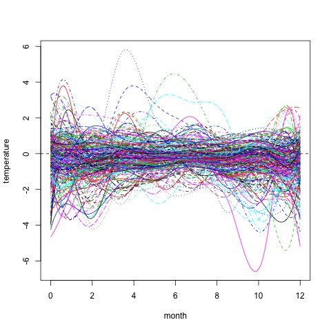
Refer to caption
Figure 1: Land-surface average temperature curves between 1753–2016
Refer to caption
Refer to caption
Refer to caption
Refer to caption
Figure 2: Land-surface average temperature curves for every 66 years
Refer to caption
Figure 3: C⁡(k)C(k) for different kk between 1753–2016
Refer to caption
Refer to caption
Figure 4: The plot on the left is the land-surface average temperature curves between 1753–1913. The plot on the right is the land-surface average temperature curves between 1914–2016.
Refer to caption
Figure 5: C⁡(k)C(k) for different kk between 1753–1913
Refer to caption
Refer to caption
Figure 6: The plot on the left is the land-surface average temperature curves between 1753–1838. The plot on the right is the land-surface average temperature curves between 1839–1913.
Refer to caption
Figure 7: C⁡(k)C(k) for different kk between 1914–2016
Refer to caption
Refer to caption
Figure 8: The plot on the left is the land-surface average temperature curves between 1914–1968. The plot on the right is the land-surface average temperature curves between 1969–2016.
{forest}
Figure 9: Subgroups between 1753–2016

References

  • Abramovich et al. (1998) Abramovich, F., Sapatinas, T., and Silverman, B. W. (1998). “Wavelet thresholding via a Bayesian approach.” Journal of the Royal Statistical Society. Series B, 60: 725–749.
  • Antoniadis et al. (2013) Antoniadis, A., Brossat, X., Cugliari, J., and Poggi, J. (2013). “Clustering functional data using wavelets.” International Journal of Wavelets, Multiresolution and Information Processing, 11: 1350003–1350032.
  • Aston and Kirch (2012) Aston, J. and Kirch, C. (2012). “Detecting and estimating changes in dependent functional data.” Journal of Multivariate Analysis, 109: 204–220.
  • Aue et al. (2018) Aue, A., Rice, G., and Sönmez, O. (2018). “Detecting and dating structural breaks in functional data without dimension reduction.” Journal of the Royal Statistical Society. Series B, 80: 509–529.
  • Berkes et al. (2009) Berkes, I., Gabrys, R., Horváth, L., and Kokoszka, P. (2009). “Detecting changes in the mean of functional observations.” Journal of the Royal Statistical Society. Series B (Statistical Methodology), 71: 927–946.
  • Ghosal and van der Vaart (2017) Ghosal, S. and van der Vaart, A. (2017). Fundamentals of nonparametric Bayesian inference. Cambridge, UK: Cambridge University Press.
  • James and Matteson (2014) James, N. A. and Matteson, D. S. (2014). “ecp: An R package for nonparametric multiple change point analysis of multivariate data.” Journal of Statistical Software, 62(7).
  • Lian (2011) Lian, H. (2011). “On posterior distribution of Bayesian wavelet thresholding.” Journal of Statistical Planning and Inference, 141: 318–324.
  • Schwartz (1965) Schwartz, L. (1965). “On Bayes procedures.” Probability Theory and Related Fields, 4: 10–26.
  • Sharipov et al. (2016) Sharipov, O., Tewes, J., and Wendler, M. (2016). “Sequential block bootstrap in a Hilbert space with application to change point analysis.” The Canadian Journal of Statistics, 44: 300–322.
  • Suarez and Ghosal (2016) Suarez, A. and Ghosal, S. (2016). “Bayesian clustering of functional data using local features.” Bayesian Analysis, 11: 71–98.
  • Zhang et al. (2011) Zhang, X., Shao, X., Hayhoe, K., and Wuebbles, D. (2011). “Testing the structural stability of temporally dependent functional observations and application to climate projections.” Electronic Journal of Statistics, 5: 1765–1796.