Q-Hermite polynomials chaos approximation of likelihood function based on q-Gaussian prior in Bayesian inversion
Abstract
In real applications, the construction of prior and acceleration of sampling for posterior are usually two key points of Bayesian inversion algorithm for engineers. In this paper, q-analogy of Gaussian distribution, q-Gaussian distribution, is introduced as the prior of inverse problems. And an acceleration algorithm based on spectral likelihood approximation is discussed. We mainly focus on the convergence of the posterior distribution in the sense of Kullback-Leibler divergence when approximated likelihood function and truncated prior distribution are used. Moreover, the convergence in the sense of total variation and Hellinger metric is obtained. In the end two numerical examples are displayed.
Key words: q-Gaussian prior; q-Hermite polynomials; Spectral likelihood approximation; Kullback-Leibler divergence
MSC 2010: 65R32, 65R20
1 Introduction
Bayesian approach has been widely applied to inverse models and parameter inference models [11, 20, 44, 45, 48, 32, 33, 53, 54, 55, 56]. It provides a handy framework for the data analysis in the real engineering problems [3, 17, 52] based on Bayes theorem,
| (1.1) |
where the distribution characterizes prior knowledge about the unknown parameter and determines the likelihood function. In real applications, two key aspects of Bayesian method perplex engineers and researchers: the prior distribution and acceleration of simulation. Firstly, the prior information is coded before obtaining the measured data. This means that one needs to have the first understanding for the unknown parameter and make some survey according to their own experience and actual situation. However, this is usually a challenging task in some real problems, e.g., reservoir, non-destructive inspection, CT etc. This prompts us to explore broader and more suitable prior distributions for specific problems. In [44, 45], some prior distributions, e.g., Gauss, uniform, Besov prior, have been discussed for ill-posed operator equations. We will introduce q-Gauss distribution, q-analogy of Gauss distribution, into the research of inverse problems in this paper. In what follows, more information of q-Gauss distribution will be provided. On the other hand, in the Bayesian framework parameters are frequently estimated by Markov chain Monte Carlo(MCMC) sampling techniques which typically have slow convergence. In fact, MCMC methods evaluate sequentially the posterior probability density at many different points in the parameter space, in which the forward model needs to be solved for each sample parameter to determine the likelihood function. This requires a computationally intensive undertaking (e.g., the solution of a system of PDEs). Therefore, numerical acceleration algorithm is key for real applications. A kind of important acceleration methods is to reduce computational cost in solving a statistical inverse problems [13]: reducing the cost of forward simulations, reducing the dimension of the input space and reducing the number of samples.
Q-Gaussian distribution, as an analogy to Gaussian distribution, has been discussed by many authors (see [7, 5, 6, 24] and references there), and widely used in quantum physics [41, 42]. In classical probability, the central limit theorem shows that the standardized sum of classically independent identifically distributed random variables converges to a Gaussian random variable as goes to infinity. This process depends on the commutative notion of independence. However, this conventional commutative relation is unsuitable for some real applications. Some necessary extensions need to be done. In [5], Bożjko and Speicher generalize the commutative independence in a deformation of Brownian motion by introducing a parameter . When , it is the classical case, the anti-commutative independence and the free independence. These commutative notions are used to characterize some quantum physics phenomena [30, 35, 43, 49]. The density function of q-Gaussian distribution is represented by an infinite series and this truncation error of the partial sum series is discussed in [47]. Compared with classical Gaussian random variables, q-Gaussian variables for are bounded, with which we can depict some bounded physical parameters, e.g., the diffusion coefficients in heat conduction problems, the order of fractional diffusion equation. In addition, with big (greater than some constant ), the density functions of q-Gaussian distribution are unimodal. While is small, they are bimodal. Bimodal probability distributions have important applications in economic, natural problems. For more discussions about q-Gaussian distribution, one can refer to [5, 6, 47].
Numerical acceleration has been always concerned by scientists and engineers. As stated above, in statistical inference problems, the main acceleration ideas include improving the sampling efficiency, reducing the dimensionality of input parameter and reducing the evaluation cost of the forward problem. In improving sampling efficiency, one can see [8, 9, 18, 12]. In [9], Cui et al integrate the reduced-order model construction process into an adaptive MCMC algorithm, in which the reduced-order model is used to increase the efficiency of MCMC sampling. For reducing the dimensionality, ad hoc method is to expand the unknown parameter in its Karhunen-Loéve expansion according to the given prior knowledge [11, 44] and truncate the expansion into the partial sum. The expansion coefficients of the truncation series are viewed as the substitute of the unknown. For reducing the evaluation cost of the forward problem, one usually tries to transform complex forward models into a simplified or coarsed version, e.g., model reduction method, or construct an approximation or ’surrogate’ of the forward problem. A lot of research has been devoted to these fields, for instance, some model reduction and surrogate based approaches [1, 13, 14, 19, 26, 31], generalized polynomial chaos (gPC) methods [32, 33, 34, 50, 51, 53, 54] and Gaussian process regression method [21, 39, 46]. Recently, on the basis of surrogate method of forward model, some authors propose a ’more-direct’ surrogate algorithm, spectral likelihood approximation method [37]. This approach does not replace the forward model directly, but replace the likelihood function with the orthogonal polynomials expansion. By this approach, the polynomial chaos expansion (PCE) has clearer explanation in mathematics. In this paper, we consider a spectral likelihood approximation approach based on q-Hermite polynomials, which are orthogonal with q-Gaussian distribution weight.
This paper is organized by the following: In Section 2, we introduce some basic knowledge about q-Gaussian distribution and q-Hermite polynomials. We give a convergence rate for the truncation q-Hermite polynomial expansion. In Section 3, the Bayesian inversion based on q-Gaussian prior is stated. In Section 4, we consider polynomial chaos expansion of likelihood function based on q-Hermite polynomials. In Section 5, we analyze the Kullback-Leibler divergence in two approximation process: the likelihood and the prior approximation. Two numerical examples are given in Section 6.
2 Preliminaries
In this section, we first give some basic conceptions and notations and then analyze the convergence rate for truncated q-Hermite polynomial expansion. We just discuss 1-dimensional case in this section. For multi-dimensional case, it is a direct extension.
Denote for and
| (2.1) | ||||
| (2.2) |
The density function of q-Gaussian [6] is supported by the interval , on which
| (2.3) |
with , and . The density function has the following expansion and the truncated error estimation [47] :
Lemma 2.1.
For , one has for
where is Chebyshev polynomial of the second kind defined by
Denote
Moreover for , it has the following estimation
| (2.8) |
Let and be the Hilbert space of functions that are square integrable with respect to the measure
| (2.9) |
To simplify, we set . The inner product and norm are defined by
| (2.10) | ||||
| (2.11) |
Q-Hermite polynomials [22] are determined by the following recurrence relation
| (2.12) |
with and . They are orthogonal to each other with respect to measure (2.9). We can write the orthogonal relation in the following
| (2.13) |
where and is the Kronecker delta.
Define the q-differential [22]:
| (2.14) |
where
| (2.15) | ||||
| (2.16) |
It follows for q-Hermite polynomials that [22]
| (2.17) |
and generally
| (2.18) |
For , it has the following expansion
| (2.19) |
Denote the first terms sum of (2.19) by
| (2.20) |
Following a similar proof in [2], we have the following truncated error estimation.
Proposition 2.2.
Let and . For being times continuously q-differentiable, the convergence rate
| (2.21) |
can be obtained. Especially, for , when , we have
| (2.22) |
Proof.
We assume . For , the proof is exactly same.
By the orthogonality of q-Hermite polynomials, for any , it holds the Parseval identify
| (2.23) |
Using the formulation (2.18), with some simple calculations we get
| (2.24) |
Using the above (2.23) and (2.24) we have
This completes the proof of (2.21).
Next, for ,
the q-Hermite expansion coefficients of hold
| (2.25) |
The Parseval equality (2.23) gives
| (2.26) |
The right can be rewritten as
| (2.27) |
Remark 1.
For , are the Chebyshev polynomials. When has continuous derivatives, then One can refer [15] for more details.
3 Bayesian inversion based on q-Gaussian prior
Inverse problems are to find , an input to a mathematical model, from given observation . We have an equation of the form
| (3.1) |
where is the data noise, is the true solution and is the forward operator, are Banach spaces. To simplify the discussion, we assume to be finite dimensional spaces . The most common used method to solve (3.1) is regularization techniques, e.g., Tikhonov regularization that searches the minimizer of the following minimization problem
| (3.2) |
where is the prior guess.
In Bayesian inversion, inverse problem (3.1) is restated within probability framework. In details, we consider as sample spaces. Let be a random variable in and be a realization of (In subsequent, we denote random variables by capital letters and its realization by the corresponding lower letters.). The forward operator maps probability space to probability space . Here and with the subscripts denote the Borel -algebras and the probability measures in the corresponding space respectively (We omit the subscripts under no any confusion). Instead of finding an estimation from an observation , we explore the probability distribution of random variable given by . According to Bayes’ formula (1.1), it is transformed to determine likelihood function and prior distribution. We take the distribution of noise as the Gaussian, i.e.,
| (3.3) |
where is the noise covariance matrix. In this case, the likelihood function can be written as
| (3.4) |
where det denotes the determinant. We assume that the components of the uncertain parameter vector are independent random variables . For each component, we set its prior density as the q-Gaussian defined by (2.9) with mean and variance . For multi-dimensional case, with a slight abuse of notation, we still denote the measure by for multi-dimensional case. Therefore, the posterior density satisfies
| (3.5) |
Maximizing the posterior probability is equivalent to minimizing the following function
| (3.6) |
where is the negative log likelihood, also called the potential function. By the i.i.d. of , we get the Hessian matrix of
where
Lemma 3.1.
[47] is bimodal for , where is the largest real root of the equation .
The fact that for is unimodal implies that and therefore is positive semidefinite, which means that is a convex penalty term of function (3.6). Whereas, when , there exists three extreme points . It is obvious that and , . Moreover, because is probability density function, it satisfies that . Thereby, we have and , which implies is a non-convex penalty function. For non-convex constraint, the function (3.6) has multi local minima. This case is typically hard to solve and analyze in classical optimization framework.
4 Polynomial chaos expansion of likelihood function based on q-Hermite polynomials
4.1 Spectral likelihood approximation
We know that q-Hermite polynomials are orthogonal with respect to measure . Define multivariate polynomials
| (4.1) |
where . It is obvious that polynomials are orthogonal with respect to measure in (2.9)
| (4.2) |
Polynomials form a complete orthogonal system of . The likelihood function is measurable in the prior measure . It can be expanded in
| (4.3) |
where is the Fourier coefficients depending on data defined by
| (4.4) |
In real numerical implementation, the expansion in (4.3) will be truncated to a finite summation
| (4.5) |
where is finite multi-indices set defined by
| (4.6) |
This truncation means that we need collect all multivariate polynomials with order smaller than or equal to . The total number [37, 53, 54] is
A simple way to reduce the dimension is to limit the number of regressors relies on hyperbolic truncation sets. For a quasinorm is defined as . The corresponding hyperbolic truncation scheme is then given as The convergence in the mean-square sense is indicated in [4, 37]
| (4.9) |
If is times continuous q-differentiable about , Theorem 2.2 shows the mean square error . One can refer to [2, 36] for truncation errors for polynomial chaos expansions.
4.2 Christoffel least square
For obtaining the expansion coefficients , we adopt the stochastic collocation algorithm [33, 53]. The collocation equation will be solved in the least-square procedure. For given data , we need find the minimizer
| (4.10) |
where is a sample of , i.e., and is the sample number. In general, the sample number is greater than the number in (4.1), which leads to an overdetermined linear system
| (4.11) |
where is a Vandermonde-like matrix, and . The popular techniques for solving (4.10) include interpolatory approaches, compressive sampling or regularization and the least-squares regularization. A new approach, called Christoffel least-squares, is proposed in [38]. This method takes to be i.i.d. from another distribution . Let be the density function of . The support of contains the support of . Instead of least-squares problem (4.10), we solve
| (4.12) |
where . Obviously, the solution is defined by
| (4.13) |
where is a diagonal matrix with entries and are defined like in (4.11) by replacing the samples drawn from distribution . The solution can be obtained by solving the normal equation of (4.13)
| (4.14) |
The CLS algorithm choose the weights to be quantities that scale each row of to have norm equal to the constant , i.e.,
| (4.15) |
The measure is called pluripotential equilibrium measure, which has density function for our settings, i.e., the q-Gaussian density
| (4.16) |
This is Chebyshev density corresponding to the arcsin measure. The equilibrium measure for multi-dimensional case is the product of the univariate measure for i.i.d. case.
5 Convergence analysis
In this section, we analyze the error between the exact posterior measure
| (5.1) |
and its approximation version
| (5.2) |
where is defined by replacing in (2.9) with its truncated version . In addition, we introduce the measure
| (5.3) |
We will focus on the Kullback-Leibler (KL) divergence [28, 29, 32, 40] (also known as the relative entropy) of with respect to to measure the bound
| (5.4) |
where means is absolutely continuous with respect to . If and are two measures on a -algebra of subsets of , we say that is absolutely continuous with respect to if for any such that . If the measure is finite, i.e. , the property is equivalent to the following stronger statement: for any there is a such that for every with . The Kullback-Leibler divergence is vital in measuring the loss of information when is instead of in information theory. As seen in [40], the Kullback-Leibler divergence is non-negative. But, since it may not meet the symmetric and the triangle inequality, it is not a metric on the space of probability measures. Nevertheless, we can use it to quantify the proximity of the measures and by virtue of some inequalities like
| (5.5) |
and
| (5.6) |
where are the so-called total variation metric and Hellinger metric respectivelly.
For convenience, we assume the noise covariance .
Assumption 1.
Lemma 5.1.
By the above assumption and Lemma 5.1, we have the following convergence result.
Theorem 5.2.
Proof.
According to the non-negative of the relative entropy, we get
Since , we know , which yields
| (5.8) |
Here
| (5.9) |
When , we get by Lemma 5.1
| (5.10) | ||||
| (5.11) |
for . When , we have almost everywhere. In fact, according to the convergence
| (5.12) |
we have for arbitrary , there exists , when
| (5.13) |
Define and . If
then we have
| (5.14) | ||||
The arbitrary of leads to a contradiction. Therefore, we can assume . Likewise, since likelihood function is non-negative for any , we also suppose . By this, it follows that
| (5.15) |
For , we have
So long as is sufficient large, we can guarantee for . In fact, is greater than that assure can meet this point. The boundedness of from below can be obtained by the similar reasons.
| (5.16) | ||||
Therefore, we have
| (5.17) |
which yields
| (5.18) |
∎
Moreover, using Lemma 2.1, we get
Theorem 5.3.
When , we have
| (5.19) |
Proof.
We only analyze the case of . For , the independence of each components of yields the same discussion. As the discussion in Theorem 5.2, it follows that
| (5.20) | ||||
Denoting , we write
| (5.21) |
By the expressions of and , the common factor contains two null points, which are all the zero points of and . And the remainder factors of them have no zero points, which yields according to Lemma 2.1
Thus as . This gives our conclusion. ∎
Corollary 5.4.
The same conditions as in Theorem 5.2 hold. We have for
| (5.26) | |||
| (5.27) |
6 Numerical test
In the numerical examples, we implement the Metropolis-Hastings algorithm [44] to sample from the posterior distribution. This algorithm aims at sampling from a target distribution with density . Algorithm MH provides the details of this algorithm.
| Algorithm MH: Metropolis-Hastings algorithm |
| Initialize |
| for do |
| Propose: Move to a candidate |
| according to a transition density . |
| Acceptance probability: |
| . |
| Uniform. |
| Accept the proposal with probability , i.e., |
| end for |
6.1 1D problem
We consider the estimation problem of the unknown mean according to random realizations , which are drawn independently from a Gaussian distribution with a given standard deviation . It can be seen that if the prior is taken as Gaussian distribution, the posterior is also Gaussian. Here we suppose that obeys a q-Gaussian prior distribution. The posterior distribution exhibits non-Gaussianity. We use this simple example as the first testbed. The likelihood function can be written as
Thereby, we get the posterior according to Bayes’ formula
We generate the data from Gaussian distribution with the true mean and the standard deviation . For the numerical experiment, the pseudo-random numbers
are used as synthetic data. In the Christoffel algorithm, the density function for the pluripotential equilibrium measure is taken as
| (6.1) |
The parameter and are specified as and with a fixed positive constant . In the numerical tests, the prior density is truncated to the first terms, i.e., . The normalization constants and (has a similar definition with ) are computed by Monte Carlo method. We list the relative error of the posterior density function in Table 1. The results show that the spectral likelihood expansion (SLE) approximation can fit the likelihood function well and the numerical precision is higher with higher order polynomial. For comparison purposes, we draw some samples from the posterior distribution by means of MCMC. An independence sampling process is utilized. The likelihood function and its SLE approximation, the posterior density and a normalized histogram of the obtained random walk samples are shown in Fig. 1. From the results, it can be seen that the SLEs are able to approximate the likelihood function well. As depicted in [37], these well-fitted regions accumulate the largest proportions of the total prior probability mass. Due to the reason that the q-Gaussian priors have compact, even though the SLEs start strongly deviating from the likelihood function, the posterior densities by using SLEs vanish when far away from the peaks. From the viewpoint, the proposed priors are better options for fitting the posterior densities by using SLEs. For the sampling effect, the histogram plots can reflect the posterior densities well.
| -0.5 | 0.0772 | 0.0065 | 0.0044 | 1.8092e-04 | 6.8778e-05 |
| -0.2 | 0.0963 | 0.0077 | 0.0048 | 1.9242e-04 | 9.2320e-05 |
| 0 | 0.1083 | 0.0088 | 0.0061 | 1.9865e-04 | 5.1662e-05 |
| 0.2 | 0.1202 | 0.0097 | 0.0069 | 2.3369e-04 | 6.0067e-05 |
| 0.5 | 0.1627 | 0.0120 | 0.0085 | 2.6809e-04 | 7.0980e-05 |


6.2 2D problem
We consider a stationary inverse heat conduction problem governed by
| (6.2) | ||||
| (6.3) | ||||
| (6.4) |
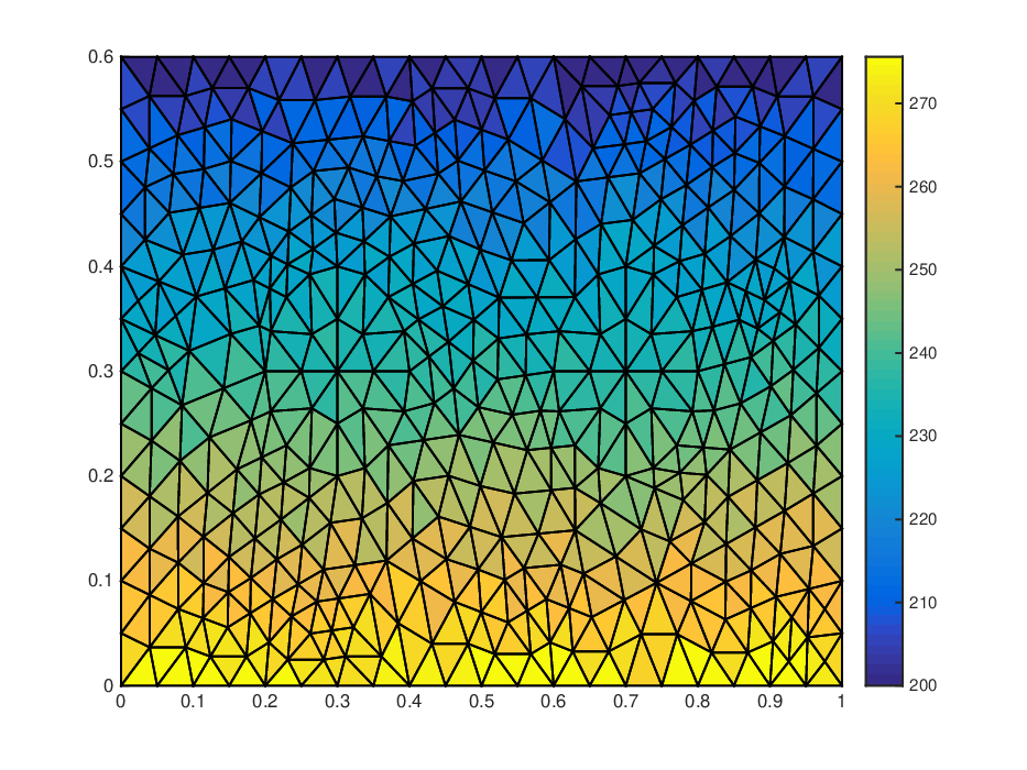
where with boundary , takes different values at and are the given functions. For the test example, we use the same settings as in [37], where is a square domain and . The subdomains are disks located at with radius respectively. The Dirichlet boundary condition and Neumann boundary conditions . The forward problem is to find the solution for given . The inverse heat conduction problem is to seek by measurements of at some fixed points in domain . The domain settings are displayed in Fig. 2. The forward problem is solved in linear finite element method and we show the finite element solution in Fig. 3. The data is acquired at scattered points distributed in the domain by adding absolute error to the numerical solution of the forward problem, i.e.,
where is the 10 measure point position vector. We display several numerical effects in Fig. 4 for different and noise . The results show that when is smaller, the peak of posterior density is closer to the true value. And the MCMC samples can reflect the posterior density well. However, there exists some differences away from the peak between the posterior density with the SLE and the original model. This also leads to some samples do not concentrate close to the peak.


Conclusions
We have introduced a new prior model, namely, q-Gaussian prior, into the research of inverse problems, which is q-analogue of classical Gaussian distribution. Since the density function of each q-Gaussian distribution has compact support, we can characterize some bounded physical parameters using it. In order to accelerate the computation of MCMC sampling in Bayesian inversion, we adopted a spectral likelihood approximation algorithm based on q-Hermite polynomial chaos expansion of likelihood function. Then we proved the convergence of posterior distribution in the framework of relative entropy when the likelihood function is replaced with truncated PCE. And when the q-Gaussian prior is approximated, we also studied the convergence of the corresponding approximated posterior measure. With the proposed prior and SLE algorithm, we verified the effectiveness of the proposed method through two numerical examples .
References
- [1] S. Arridge, J. Kaipio, V. Kolehmainen, M. Schweiger, E. Somersalo, T. Tarvainen and M. Vauhkonen, Approximation errors and model reduction with an application in optical diffusion tomography, Inverse Problems 22, 175-195, 2006.
- [2] F. Augustin, A. Gilg, M. Paffrath, P. Rentrop and U. Wever, A survey in mathematics for industry, Polynomial chaos for the approximation of uncertainties: chances and limits, Euro. Jnl of Applied Mathematics, 19, 149-190, 2008.
- [3] J. L. Beck, Bayesian system identification based on probability logic, Struct. Control Health Monit. 17(7) (2010) 825-847.
- [4] G. Box and N. Draper, Response Surfaces, Mixtures, and Ridge Analyses, 2nd edition, Wiley Series in Probability and Statistics, John Wiley Sons, Inc., Hoboken, New Jersey, USA, 2007.
- [5] M. Bożjko and R. Speicher, An example of a generalized Brownian motion, Communications in Mathematical Physics 137, 519-531, 1991.
- [6] M. Bożjko, B. Kümmerer and R. Speicher, q-Gaussian processes: non-commutative and classical aspects, Communications in Mathematical Physics, 185(1997) 129-154.
- [7] W. Bryc, Classical Versions of q-Gaussian Processes: Conditional Moments and Bell’s Inequality, Communications in Mathematical Physics, 219, 259-270 (2001).
- [8] J. Christen and C. Fox, MCMC using an approximation, Journal of Computational and Graphical Statistics 14(4), 795-810, 2005.
- [9] T. Cui, Y. M. Marzouk and K. E. Willcox, Data-driven model reduction for the Bayesian solution of inverse problems, International Journal for numerical methods in engineering, (2014).
- [10] W. J. Cody, A survey of practical rational and polynomial approximation of functions, SIAM Review, 12(3), 1970.
- [11] M. Dashti and A. M. Stuart, The Bayesian approach to inverse problems, arXiv:1302.6989.
- [12] Y. Efendiev, T. Hou and W. Luo W, Preconditioning Markov chain Monte Carlo simulations using coarse-scale models. SIAM Journal on Scientific Computing 28, 776-803, 2006.
- [13] M. Frangos, Y. Marzouk, K. Willcox and B. van Bloemen Waanders, Surrogate and reduced order modeling: a comparison of approaches for large-scale statistical inverse problems Computational Methods for Large Scale Inverse Problems and Uncertainty Quantification ed L Biegler et al (New York: Wiley) pp 123-149, 2010.
- [14] D. Galbally, K. Fidkowski, K. Willcox and O. Ghattas, Non-linear model reduction for uncertainty quantification in large-scale inverse problems, Int. J. Numer. Methods Eng. 81, 1581-1608, 2010.
- [15] A. Gil, J. Segura and N. Temme, Numerical Methods for Special Functions, SIAM, 2007.
- [16] Y. Hatano, J. Nakagawa, S. Wang and M. Yamamoto, Determination of order in fractional diffusion equation, Journal of Math-for-Industry, 5(2013A-7), 51-57.
- [17] R. Hadidi, N. Gucunski, Probabilistic approach to the solution of inverse problems in civil engineering, J. Comput. Civ. Eng. 22(6) (2008) 338-347.
- [18] D. Higdon, H. Lee and C. Holloman, Markov chain Monte Carlo-based approaches for inference in computationally intensive inverse problems, Bayesian Statistics 7, 181-197, 2003.
- [19] B. Jin, Fast Bayesian approach for parameter estimation Int. J. Numer. Methods Eng. 76, 230-252, 2008.
- [20] J. Kaipio and E. Somersalo, Statistical and Computational Inverse Problems, vol. 160 of Applied Mathematical Sciences, Springer, 2005.
- [21] M. Kennedy and A. O’Hagan, Bayesian calibration of computer models, J. R. Stat. Soc.: Ser. B, 63, 425-464, 2001.
- [22] R. Koekoek, P. Lesky and R. Swarttouw, Hypergeometric Orthogonal Polynomials and Their q-Analogues, Springer-Verlag Berlin Heidelberg, 2010.
- [23] J. Koekoek and R. Koekoek, A note on the q-derivative operator, Journal of Mathematical Analysis and Applications, 176, 627-634, 1993.
- [24] H. van Leeuwen and H. Maassen, A q deformation of the Gauss distribution, Journal of Mathematical Physics 36, 4743-4756, 1995.
- [25] Z. Li and M. Yamamoto, Uniqueness for inverse problems of determining orders of multi-term time-fractional derivatives of diffusion equation, Applicable Analysis, 94(3), 570-579, 2015.
- [26] C. Lieberman, K. Willcox and O. Ghattas, Parameter and state model reduction for large-scale statistical inverse problems SIAM J. Sci. Comput. 32, 2523-2542, 2010.
- [27] F. Liu, P. Zhuang, V. Anh and I. Turner, A fractional-order implicit difference approximation for the space-time fractional diffusion equation, ANZIAM J. 47 (EMAC2005) pp.C48šCC68, 2006
- [28] Y. Lu, A. Stuart and H. Weber, Gaussian approximations for probability measures on , SIAM/ASA J. Uncertainity Quantification, 5, 1136-1165, 2017.
- [29] Y. Lu, A. Stuart and H. Weber, Gaussian approximations for transition paths in Brownian dynamics, SIAM J. Math. Anal., 49(4), 3005-3047, 2017.
- [30] H. Maassen, Addition of freely independent random variables, J. Funct. Anal. 106, 409-438 (1992).
- [31] A. Manzoni, S. Pagani and T. Lassila, Accurate solution of Bayesian inverse uncertainty quantification problems combining reduced basis methods and reduction error models SIAM/ ASA J. Uncertain. Quantification 4, 380-412, 2016.
- [32] Y. Marzouk, N. Habib and L. Rahn, Stochastic spectral methods for efficient Bayesian solution of inverse problems, Journal of Computational Physics 224, 560-586, 2007.
- [33] Y. Marzouk and D. Xiu, A stochastic collocation approach to Bayesian inference in inverse problems, Communications in Computational Physics 6, 826-847, 2009.
- [34] Y. Marzouk and H. Najm, Dimensionality reduction and polynomial chaos acceleration of Bayesian inference in inverse problems, Journal of Computation Physics, 228, 1862-1902.
- [35] P. Meyer, Quantum probability for probabilists, Vol. 1538 of Lecture Notes in Mathematics (Springer-Verlag, Berlin, 1993).
- [36] T. Mühlpfordt, R. Findeisen and T. Faulwasser, Comments on truncation errors for polynomial chaos expansions, IEEE control systems letters, 2(1), 169-174, 2018.
- [37] J. B. Nagel and B. Sudret, Spectral likelihood expansions for Bayesian inference, Journal of Computational Physics 309 (2016) 267-294.
- [38] A. Narayan, J. Jakeman and T. Zhou, A Christoffel function weighted least squares algorithm for collocation approximations, Mathematics of Computation, 86(306), 1913-1947, 2017.
- [39] C. Rasmussen, J. Bernardo, M. Bayarri, J. Berger, A. Dawid, D. Heckerman, A. Smith and M. West, Gaussian processes to speed up hybrid Monte Carlo for expensive Bayesian integrals, Bayesian Statistics, 7, J. Bernardo et al (Oxford: Oxford University Press) 651-659, 2003.
- [40] Gaussian approximations of small noise diffusions in Kullback-Leibler divergence, Commun. Math. SCI., 15(7), 2087-2097, 2017.
- [41] B. Simon, The Euclidean (Quantum) Field Theory. Princeton, NJ: Princeton University Press, 1974.
- [42] B. Simon, Functional Integration and Quantum Physics. New York: Academic Press, 1979.
- [43] R. Speicher, A new example of independence and white noise, Prob. Theory Rlated Fields 84, 141-159 (1990).
- [44] A. M. Stuart, Inverse problems: A Bayesian perspective, Acta Numerica. 19 (2010), 451-559.
- [45] A. M. Stuart, The Bayesian approach to inverse problems, Lecture Notes, arXiv:1302.6989.
- [46] A. Stuart and A. Teckentrup, Posterior consistency for Gaussian process approximations of Bayesian posterior distributions, Math. Comput. 87(310), 721-753, 2018.
- [47] P. Szablowski, q-Gaussian distributions: simplifications and simulations, Journal of Probability and Statistics 2009, Article ID 752430, 18 pages.
- [48] A. Tarantola, Inverse Problem Theory and Methods for Model Parameter Estimation, SIAM, 2005.
- [49] D. Voiculescu, K. Dykema, and A. Nica, Free random variables, Vol. 1 of CRM Monograph Series (American Mathematical Society, Providence, RI, 1992).
- [50] D. Xiu, Numerical Methods for Stochastic Computations. Princeton University Press, 2010.
- [51] D. Xiu and G. Karnianakis, The Wiener-Askey polynomial chaos for stochastic differential equations, SIAM J. Sci. Comput., 24(2), 619-644, 2002.
- [52] K.-V. Yuen, S.-C. Kuok, Bayesian methods for updating dynamic models, Appl. Mech. Rev. 64(1) (2011) 010802, 1-18.
- [53] L. Yan and L. Guo, Stochastic collocation algorithms using minimization for Bayesian solution of inverse problems, SIAM J. Sci. Comput. 37(3) (2015), A1410-A1435.
- [54] L. Yan and Y. Zhang, Convergence analysis of surrogate-based methods for Bayesian inverse problems, Inverse Problems 33, 125001 (20pp), 2017.
- [55] L. Yan, F. L. Yang and C. L. Fu, A Bayesian inference approach to identify a Robin coefficient in one-dimensional parabolic problems, Journal of Computational and Applied Mathematics 231(2) (2009), 840-850.
- [56] X. Yang and Z. Deng, A data assimilation process for linear ill-posed problems, Mathematical methods in the applied sciences 40(16) (2017), 5831-5840.