跳到论文正文
W Papers独立论文阅读器 arXiv:1808.00927 论文正文 计算阅读时间 · 0%
引用这篇论文根据当前论文元数据生成,正式投稿前建议核对。


License: arXiv.org perpetual non-exclusive license
arXiv:1808.00927v1 [quant-ph] 02 Aug 2018

Coherent spin-wave processor of stored optical pulses

Mateusz Mazelanik Email: mateusz.mazelanik@fuw.edu.pl Affiliation: Faculty of Physics, University of Warsaw, Pasteura 5, 02-093 Warsaw, Poland    Michał Parniak Email: michal.parniak@fuw.edu.pl Affiliation: Faculty of Physics, University of Warsaw, Pasteura 5, 02-093 Warsaw, Poland    Adam Leszczyński Affiliation: Faculty of Physics, University of Warsaw, Pasteura 5, 02-093 Warsaw, Poland    Michał Lipka Affiliation: Faculty of Physics, University of Warsaw, Pasteura 5, 02-093 Warsaw, Poland    Wojciech Wasilewski Affiliation: Faculty of Physics, University of Warsaw, Pasteura 5, 02-093 Warsaw, Poland
Abstract

A device being a pinnacle of development of an optical quantum memory should combine the capabilities of storage, inter-communication and processing of stored information. In particular, the ability to capture a train of optical pulses, interfere them in an arbitrary way and finally perform on-demand release would in a loose sense realize an optical analogue of a Turing Machine. Here we demonstrate the operation of an optical quantum memory being able to store optical pulses in the form of collective spin-wave excitations in a multi-dimensional wavevector space. During storage, we perform complex beamsplitter operations and demonstrate a variety of protocol implemented as the processing stage, including interfering a pair of spin-wave modes with 95% visibility. By engineering the phase-matching at the readout stage we realize the on-demand retrieval. The highly multimode structure of the presented quantum memory lends itself both to enhancing classical optical telecommunication as well as parallel processing of optical qubits at the single-photon level.

I Introduction

As optical quantum memory technologies are becoming more mature, the range of of their applications increases. The basic memories operating in a single temporal and spatial mode can store only one optical pulse and interfere it with second pulse only during light-atom coupling [1]. Such memories, based either on Raman scattering or electromagnetically induced transparency (EIT), can achieve high efficiencies [2], but offer very limited capacity as multiplexing is limited by the number of atomic magnetic sublevels employed [3, 4, 2, 5]. While a single atomic ensemble may be split into an array to offer parallel storage of light [6, 7], such scheme hinders manipulations within the memory as communication between memory cells must be inherently light-based. It is thus highly desirable to independently store many optical pulses within the same group of atoms. Such a multiplexing scheme may utilize either the spatial [8, 9] or temporal degree of freedom [10, 11, 12]. In the latter case considered in the context of the atomic-ensemble based quantum memories the Gradient Echo Memory (GEM) [13, 14, 15, 16, 17] scheme stands out as an efficient way to engineer the phase-matching at readout stage to achieve mode-selective storage and retrieval. Similar feature is inherently offered by the atomic frequency comb (AFC) memories based on ensembles of ions in solids [11, 10, 18] thanks to their large inhomogeneous broadening. In the spatial degree of freedom atomic ensembles allow storage of light in many angular-emission modes through spin-wave wavevector multiplexing [19, 8]. These schemes allow storage of hundreds of optical modes, also when used with non-classical states of light.

Manipulation of stored optical pulses, however, remains a substantial challenge, both from technical and fundamental points of view. The AFC memory has been demonstrated to allow pre-programmed interference of two stored pulses with a single-output port [20, 21], and within the GEM scheme a beamsplitter operation between a pre-selected stored pulses and an input pulse has been realized [22, 23]. These schemes also allow basic spectral and temporal manipulations of stored light. More work is needed however to reach the regime of efficient and arbitrary manipulations of stored light. In particular, the ac-Stark shift caused by an additional light field has been proposed as a versatile way to realize the GEM scheme [24]. Recent theoretical proposals went beyond the simple gradient shape and suggested to engineer the stored spin-wave shape to realize Kapitsa-Dirac diffraction [25] or a quantum memory protected with a disordered password [26]. Finally, a recent experiment used the ac-Stark shift to realize a spin-wave beamsplitter at the single-excitation level demonstrating Hong-Ou-Mandel interference for stored light [27].

Here we present the first realization of ac-Stark-based spin-wave universal multiport interferometric processor (SUMIP) and join the advantages of the transverse-wavevector and temporal multiplexing to realize a variety of operations on the stored coherent states of light. The previously untackled regime of complex light patterns used to engineer spin waves is explored, which allows us to tap into the full three-dimensional potential of the wavevector-multiplexed optical quantum memory. We show that thanks to engineering of the spatial profile of ac-Stark modulation the stored pulses may be processed, interfered and conditionally retrieved. The scheme features both reprogrammable reordering and interference of pulses within the multiple-input, multiple-output paradigm, essential to realize true unitary operations. In the paper we first introduce the protocol by deriving its theoretical principles and realizing a scheme reminiscent of the Gradient Echo Memory [14]. Next, we realize a series of programmable beamsplitting experiments in spatial and temporal degrees of freedom. High-visibility interference of a pair of modes is demonstrated. Finally, we propose potential further applications and give technical details of the experiment and light-atom propagation simulations involved.

II Operation of the light-atom interface

The atomic optical memory based on an elongated ensemble of Rb-87 atoms employs a strong control field ℰC\mathcal{{E}}_{C} to map a weak signal field ℰi​n\mathcal{{E}}_{in} onto the atomic coherence ρg​h\rho_{gh} between the two meta-stable ground states, for which we take |g⟩→|g\rangle\rightarrow F=1,mF=−1F=1,\ m_{F}=-1, and |h⟩→|h\rangle\rightarrow F=2,mF=1F=2,\ m_{F}=1 (see Fig. 1c for the atomic level scheme). In the experiment the atoms are first optically pumped to the |g⟩|g\rangle state and control and signal fields operate with opposite circular polarizations. Typically we use 300 ns long pulses for storage and retrieval of atomic coherence.

While the interaction is well characterized by a set of coupled Maxwell-Bloch equations (see Appendix A), first we rather choose to describe the atom-light coupling qualitatively. In particular, Fig. 1b illustrates the geometry in which the coupling and signal fields co-propagate through an elongated atomic ensemble. Assuming that the coupling beam diameter is significantly larger than the transverse size of the ensemble, we may actually solve the coupled equations within the first order in the coupling strength and obtain a simple result by which a signal ℰ⁡(kx,ky)\mathcal{E}(k_{x},k_{y}) couples to an atomic coherence

ρg​h​(Kx,Ky,Kz)∝ℰi​n​(kx=Kx,ky=Ky)​exp⁡(i​Δ0​t)​δ​(Kz​0−Kz),\rho_{gh}(K_{x},K_{y},K_{z})\propto\\ \mathcal{{E}}_{in}(k_{x}=K_{x},k_{y}=K_{y})\exp(i\Delta_{0}t)\delta(K_{z0}-K_{z}),

where Kz​0=ω2/c2−kx2−ky2−ωC/cK_{z0}=\sqrt{\omega^{2}/c^{2}-k_{x}^{2}-k_{y}^{2}}-\omega_{C}/c, δ\delta is a Dirac delta function and ω\omega and ωC\omega_{C} are frequencies of signal and coupling fields, respectively, and cc is the speed of light. For kx=ky=0k_{x}=k_{y}=0 the longitudinal wavevector simplifies to a constant component Kz​0=c/Δ0≈0.14​rad​mm−1K_{z0}=c/\Delta_{0}\approx 0.14\ \mathrm{rad}\ \mathrm{m}\mathrm{m}^{-1}, where Δ0≈2​π×6.8​GHz\Delta_{0}\approx 2\pi\times 6.8\ \mathrm{{GHz}} is the nominal frequency splitting between levels |g⟩|g\rangle and |h⟩|h\rangle. To exclude these trivial dependencies from further consideration we will define the stored spin-wave excitation as

S(Kx,Ky,Kz)=ρg​h(Kx,Ky,Kz)∗ℱ⁡[N⁡(x,y,z)]​(Kx,Ky,Kz−Kz​0)​exp⁡(−i​Δ0​t),S(K_{x},K_{y},K_{z})=\rho_{gh}(K_{x},K_{y},K_{z})\ast\\ \mathscr{F}[\sqrt{N(x,y,z)}](K_{x},K_{y},K_{z}-K_{z0})\exp(-i\Delta_{0}t),

where ℱ\mathscr{F} stands for the Fourier transform in the spatial domain, N⁡(x,y,z)N(x,y,z) is the atom number density and ∗\ast denotes convolution (here in the wavevector space). Importantly, after mapping the optical field we obtain a spin-wave excitation with Kz=0K_{z}=0 in terms of SS.

The process of reverse mapping or retrieval driven by the same coupling field occurs in a symmetric way. Essentially, an atomic spin-wave excitation will be mapped onto an optical field proportional to SS in terms of the transverse wavevector dependence only if Kz=0K_{z}=0. This requirement arises due to the phase-matching condition. In particular, the allowed spread in the KzK_{z} space is inversely proportional to the atomic cloud length σz\sigma_{z} and most importantly spin waves with large KzK_{z} component (Kz​σz≫1K_{z}\sigma_{z}\gg 1) will remain stored in the memory. This remains true unless we change the frame of reference significantly by selecting much different KxK_{x}, KyK_{y}, as the actual phase matching is satisfied on an ellipsoid in a KK space rather than a plane. Its curvature will depend on the particular geometrical configuration. Here we will remain within the regime where we may use the phase-matching planar approximation to consider which spin waves are retrievable.

III Spin-wave manipulation with the ac-Stark effect

Refer to caption
Figure 1: Spin-wave processing with ac-Stark modulation. (a) Simplified simulation of exemplary protocol implemented on SUMIP, presenting the light and spin-wave domain transformations. By manipulating the spin wave using spatially varying ac-Stark (acS) shift three pulses are stored, processed and released in reversed order. In the three-dimensional plot, the colored blobs correspond to a spin-wave density exceeding a critical value. We coloring is selected to correspond to a light pulse from which the spin wave originates. (b) Pulses are sent to SUMIP in different time-space modes, then ac-Stark manipulation is applied and at the end pulses are released. Released pulses can be detected either on Avalanche Photodiode (APD) or sCMOS camera situated in the far-field (ff) for temporal or angular resolution, respectively. (c) Rubidium-87 energy level configuration utilized for storing and processing coherent light pulses. (d) Projection of the panel (b) on perpendicular plane exposing 2-d (x,z)(x,z) ac-Stark modulation capabilities using Spatial Light Modulator (SLM).

As discussed above, only a limited space, or more precisely a thin three-dimensional volume around Kz=0K_{z}=0 plane in the wavevector space may be populated by spin waves by means of Raman interaction. To manipulate the spin waves within and beyond this volume we use an additional far off-resonant beam [marked in Fig. 1(c) as acS] that induces an additional differential ac-Stark shift between levels |g⟩|g\rangle and |h⟩|h\rangle of ΔacS\Delta_{\mathrm{acS}} that adds to Δ0\Delta_{0}. The ac-Stark beam propagating along the yy-direction is zz-polarized and red-detuned by approx. 1 GHz from the |h⟩→|e⟩|h\rangle\to|e\rangle transition and is inducing ΔacS∼\Delta_{\mathrm{acS}}\sim1 MHz ac-Stark shift with ∼100\sim 100 mW beam power. This shift causes the atomic coherence ρg​h\rho_{gh}, and thus the spin wave, to accumulate an additional phase φacS=ΔacS​T\varphi_{\mathrm{acS}}=\Delta_{\mathrm{acS}}T over the interaction time TT. Typically we use ac-Stark pulses of approx. T∼2​μ​sT\sim 2\ \mu\mathrm{s} duration. By spatially shaping the ac-Stark beam intensity IacS​(x,z)I_{\mathrm{acS}}(x,z) we induce a spatially-dependent phase shift φacS​(x,z)∝IacS​(x,y)\varphi_{\mathrm{acS}}(x,z)\propto I_{\mathrm{acS}}(x,y), which due to the geometry of the experiment is limited to two dimensions [see Figure 1(b)]. Any spin wave is then reshaped as:

S⁡(Kx,Ky,Kz)=∬(X,Z)ℱ⁡[exp⁡(i​φacS​(x,z))]​(kx,kz)S⁡(Kx+kx,Ky,Kz+kz)​d​kx​d​kz.S(K_{x},K_{y},K_{z})=\\ \iint_{(X,Z)}\mathscr{F}[\exp(i\varphi_{\mathrm{acS}}(x,z))](k_{x},k_{z})\\ S(K_{x}+k_{x},K_{y},K_{z}+k_{z})\mathrm{d}k_{x}\mathrm{d}k_{z}. (1)

A basic example is an ac-Stark analogue of the GEM, in which a phase shift linear in zz (φacS=β​zCLOSE(\varphi_{\mathrm{acS}}=\beta z) induced by a magnetic field gradient shifts the spin wave in the KzK_{z} direction by β\beta.

Refer to caption
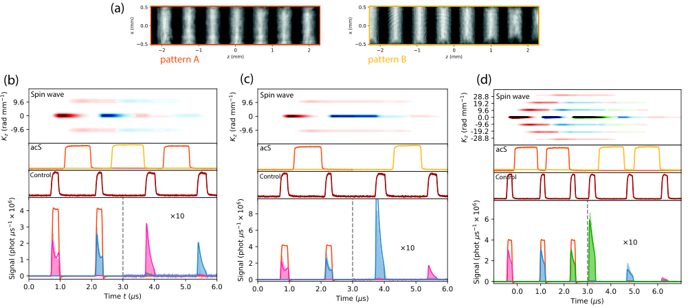
Figure 2: Operation of the ac-Stark Echo Memory. Panel (a): ac-Stark triangle-wave () modulation patterns for storage (pattern A) retrieval (pattern B) of subsequent pulses. Pattern B is a shifted by a half of a period version of pattern A with the same amplitude. Storage and retrieval of two coherent optical pulses in the last-in, first-out (LIFO) as well as first-in, first-out (FIFO) configurations [panels (b) and (c), respectively] and the LIFO configuration for storage of three pulses [panel (d)].

Here we work with optical modes characterized by small wavevector (angular) spread and therefore the spin waves are well-localized in the wavevector space. Discrete mode transformation in such a space are most conveniently performed by a spatially periodic ac-Stark modulation. Taking a spatial period 2​π/kacS2\pi/k_{\mathrm{acS}} of the modulation in the form φacS​(x,z)=φacSperiodic​(𝐤acS⋅(x,z))\varphi_{\mathrm{acS}}(x,z)=\varphi_{\mathrm{acS}}^{\mathrm{periodic}}(\mathbf{k}_{\mathrm{acS}}\cdot(x,z)) we may express the spin-wave transformation using Fourier series as:

S⁡(𝐊)→φacS​(x,z)∑n=−∞+∞cn​S​(𝐊+n​𝐤acS),S(\mathbf{K})\xrightarrow{\varphi_{\mathrm{acS}}(x,z)}\sum_{n=-\infty}^{+\infty}c_{n}S(\mathbf{K}+n\mathbf{k}_{\mathrm{acS}}), (2)

with Fourier coefficients cnc_{n} defined as:

cn=12​π​∫02​πexp⁡(i​φacSperiodic​(ξ)−i​n​ξ)​𝑑ξ.c_{n}=\frac{1}{2\pi}\int_{0}^{2\pi}\exp(i\varphi_{\mathrm{acS}}^{\mathrm{periodic}}(\xi)-in\xi)\mathrm{d\xi.} (3)

Figure 1(a) presents a simplified simulation (assuming perfect write-in and read-out) of a protocol operation within this paradigm. In this exemplary protocol three pulses ℰ0\mathcal{E}_{0}, ℰ−k\mathcal{E}_{-k}, ℰk\mathcal{E}_{k} with transverse optical wavevector component kxk_{x} equal 0, −k-k and kk, respectively, are stored, processed and released from the memory. When the first pulse is mapped to the ensemble, the created spin wave is phase-modulated using a sawtooth-shaped (periodic) modulation φacS​(x,z)=φacS      ​(k      ​z)\varphi_{\mathrm{acS}}(x,z)=\varphi_{\mathrm{acS}}^{\hbox to4.86pt{\vbox to2.59pt{\pgfpicture\makeatletter\hbox{\hskip 0.15555pt\lower-0.15555pt\hbox to0.0pt{\lxSVG@begingroup@{_scopebegin=1} \lxSVG@begingroup@{stroke=#000000} \lxSVG@begingroup@{fill=#000000} \lxSVG@setlinewidth{\the\pgflinewidth}\lxSVG@begingroup@{stroke-width=0.4pt} \lx@inpgf@ignorespaces\nullfont\hbox to0.0pt{\lxSVG@begingroup@{_scopebegin=1} {{\lx@inpgf@ignorespaces}}\lxSVG@setlinewidth{\the\pgflinewidth}\lxSVG@begingroup@{stroke-width=0.31111pt} \lx@inpgf@ignorespaces\lxSVG@rectcap\lxSVG@begingroup@{stroke-linecap=rect} \lx@inpgf@ignorespaces{ {}{{}}{} {}{} {}{} {}{} {}{} {}{}{}\lxSVG@stroke\lxSVG@drawpath@unclipped{M 0 3.15 L 0 0 L 3.15 3.15 L 3.15 0 L 6.3 3.15 L 6.3 0}{fill:none} \lx@inpgf@ignorespaces } \lxSVG@closescope {\lx@inpgf@ignorespaces}{\lx@inpgf@ignorespaces}{\lx@inpgf@ignorespaces}\hss}\lxSVG@discardpath\lxSVG@closescope \hss}}\lxSVG@closescope\endpgfpicture}}}(k_{\hbox to4.86pt{\vbox to2.59pt{\pgfpicture\makeatletter\hbox{\hskip 0.15555pt\lower-0.15555pt\hbox to0.0pt{\lxSVG@begingroup@{_scopebegin=1} \lxSVG@begingroup@{stroke=#000000} \lxSVG@begingroup@{fill=#000000} \lxSVG@setlinewidth{\the\pgflinewidth}\lxSVG@begingroup@{stroke-width=0.4pt} \lx@inpgf@ignorespaces\nullfont\hbox to0.0pt{\lxSVG@begingroup@{_scopebegin=1} {{\lx@inpgf@ignorespaces}}\lxSVG@setlinewidth{\the\pgflinewidth}\lxSVG@begingroup@{stroke-width=0.31111pt} \lx@inpgf@ignorespaces\lxSVG@rectcap\lxSVG@begingroup@{stroke-linecap=rect} \lx@inpgf@ignorespaces{ {}{{}}{} {}{} {}{} {}{} {}{} {}{}{}\lxSVG@stroke\lxSVG@drawpath@unclipped{M 0 3.15 L 0 0 L 3.15 3.15 L 3.15 0 L 6.3 3.15 L 6.3 0}{fill:none} \lx@inpgf@ignorespaces } \lxSVG@closescope {\lx@inpgf@ignorespaces}{\lx@inpgf@ignorespaces}{\lx@inpgf@ignorespaces}\hss}\lxSVG@discardpath\lxSVG@closescope \hss}}\lxSVG@closescope\endpgfpicture}}}z). Such a modulation with amplitude equal 2​π2\pi shifts the spin wave in the KzK_{z} direction by k      k_{\hbox to4.86pt{\vbox to2.59pt{\pgfpicture\makeatletter\hbox{\hskip 0.15555pt\lower-0.15555pt\hbox to0.0pt{\lxSVG@begingroup@{_scopebegin=1} \lxSVG@begingroup@{stroke=#000000} \lxSVG@begingroup@{fill=#000000} \lxSVG@setlinewidth{\the\pgflinewidth}\lxSVG@begingroup@{stroke-width=0.4pt} \lx@inpgf@ignorespaces\nullfont\hbox to0.0pt{\lxSVG@begingroup@{_scopebegin=1} {{\lx@inpgf@ignorespaces}}\lxSVG@setlinewidth{\the\pgflinewidth}\lxSVG@begingroup@{stroke-width=0.31111pt} \lx@inpgf@ignorespaces\lxSVG@rectcap\lxSVG@begingroup@{stroke-linecap=rect} \lx@inpgf@ignorespaces{ {}{{}}{} {}{} {}{} {}{} {}{} {}{}{}\lxSVG@stroke\lxSVG@drawpath@unclipped{M 0 3.15 L 0 0 L 3.15 3.15 L 3.15 0 L 6.3 3.15 L 6.3 0}{fill:none} \lx@inpgf@ignorespaces } \lxSVG@closescope {\lx@inpgf@ignorespaces}{\lx@inpgf@ignorespaces}{\lx@inpgf@ignorespaces}\hss}\lxSVG@discardpath\lxSVG@closescope \hss}}\lxSVG@closescope\endpgfpicture}}}, making the spin wave unreadable, as k      ​σz≫1k_{\hbox to4.86pt{\vbox to2.59pt{\pgfpicture\makeatletter\hbox{\hskip 0.15555pt\lower-0.15555pt\hbox to0.0pt{\lxSVG@begingroup@{_scopebegin=1} \lxSVG@begingroup@{stroke=#000000} \lxSVG@begingroup@{fill=#000000} \lxSVG@setlinewidth{\the\pgflinewidth}\lxSVG@begingroup@{stroke-width=0.4pt} \lx@inpgf@ignorespaces\nullfont\hbox to0.0pt{\lxSVG@begingroup@{_scopebegin=1} {{\lx@inpgf@ignorespaces}}\lxSVG@setlinewidth{\the\pgflinewidth}\lxSVG@begingroup@{stroke-width=0.31111pt} \lx@inpgf@ignorespaces\lxSVG@rectcap\lxSVG@begingroup@{stroke-linecap=rect} \lx@inpgf@ignorespaces{ {}{{}}{} {}{} {}{} {}{} {}{} {}{}{}\lxSVG@stroke\lxSVG@drawpath@unclipped{M 0 3.15 L 0 0 L 3.15 3.15 L 3.15 0 L 6.3 3.15 L 6.3 0}{fill:none} \lx@inpgf@ignorespaces } \lxSVG@closescope {\lx@inpgf@ignorespaces}{\lx@inpgf@ignorespaces}{\lx@inpgf@ignorespaces}\hss}\lxSVG@discardpath\lxSVG@closescope \hss}}\lxSVG@closescope\endpgfpicture}}}\sigma_{z}\gg 1. Then, two pulses with kxk_{x} components separated by 2​k2k arriving at the same time are written to the ensemble. Next, square-shaped modulation φacS​(x,z)=φacS      ​(k      ​x)\varphi_{\mathrm{acS}}(x,z)=\varphi_{\mathrm{acS}}^{\hbox to4.86pt{\vbox to2.59pt{\pgfpicture\makeatletter\hbox{\hskip 0.15555pt\lower-0.15555pt\hbox to0.0pt{\lxSVG@begingroup@{_scopebegin=1} \lxSVG@begingroup@{stroke=#000000} \lxSVG@begingroup@{fill=#000000} \lxSVG@setlinewidth{\the\pgflinewidth}\lxSVG@begingroup@{stroke-width=0.4pt} \lx@inpgf@ignorespaces\nullfont\hbox to0.0pt{\lxSVG@begingroup@{_scopebegin=1} {{\lx@inpgf@ignorespaces}}\lxSVG@setlinewidth{\the\pgflinewidth}\lxSVG@begingroup@{stroke-width=0.31111pt} \lx@inpgf@ignorespaces\lxSVG@rectcap\lxSVG@begingroup@{stroke-linecap=rect} \lx@inpgf@ignorespaces{ {}{{}}{} {}{} {}{} {}{} {}{} {}{} {}{} {}{} {}{} {}{}{}\lxSVG@stroke\lxSVG@drawpath@unclipped{M 0 0 L 0 3.15 L 1.57 3.15 L 1.57 0 L 3.15 0 L 3.15 3.15 L 4.72 3.15 L 4.72 0 L 6.3 0 L 6.3 3.15}{fill:none} \lx@inpgf@ignorespaces } \lxSVG@closescope {\lx@inpgf@ignorespaces}{\lx@inpgf@ignorespaces}{\lx@inpgf@ignorespaces}\hss}\lxSVG@discardpath\lxSVG@closescope \hss}}\lxSVG@closescope\endpgfpicture}}}(k_{\hbox to4.86pt{\vbox to2.59pt{\pgfpicture\makeatletter\hbox{\hskip 0.15555pt\lower-0.15555pt\hbox to0.0pt{\lxSVG@begingroup@{_scopebegin=1} \lxSVG@begingroup@{stroke=#000000} \lxSVG@begingroup@{fill=#000000} \lxSVG@setlinewidth{\the\pgflinewidth}\lxSVG@begingroup@{stroke-width=0.4pt} \lx@inpgf@ignorespaces\nullfont\hbox to0.0pt{\lxSVG@begingroup@{_scopebegin=1} {{\lx@inpgf@ignorespaces}}\lxSVG@setlinewidth{\the\pgflinewidth}\lxSVG@begingroup@{stroke-width=0.31111pt} \lx@inpgf@ignorespaces\lxSVG@rectcap\lxSVG@begingroup@{stroke-linecap=rect} \lx@inpgf@ignorespaces{ {}{{}}{} {}{} {}{} {}{} {}{} {}{} {}{} {}{} {}{} {}{}{}\lxSVG@stroke\lxSVG@drawpath@unclipped{M 0 0 L 0 3.15 L 1.57 3.15 L 1.57 0 L 3.15 0 L 3.15 3.15 L 4.72 3.15 L 4.72 0 L 6.3 0 L 6.3 3.15}{fill:none} \lx@inpgf@ignorespaces } \lxSVG@closescope {\lx@inpgf@ignorespaces}{\lx@inpgf@ignorespaces}{\lx@inpgf@ignorespaces}\hss}\lxSVG@discardpath\lxSVG@closescope \hss}}\lxSVG@closescope\endpgfpicture}}}x) with k      =2​kk_{\hbox to4.86pt{\vbox to2.59pt{\pgfpicture\makeatletter\hbox{\hskip 0.15555pt\lower-0.15555pt\hbox to0.0pt{\lxSVG@begingroup@{_scopebegin=1} \lxSVG@begingroup@{stroke=#000000} \lxSVG@begingroup@{fill=#000000} \lxSVG@setlinewidth{\the\pgflinewidth}\lxSVG@begingroup@{stroke-width=0.4pt} \lx@inpgf@ignorespaces\nullfont\hbox to0.0pt{\lxSVG@begingroup@{_scopebegin=1} {{\lx@inpgf@ignorespaces}}\lxSVG@setlinewidth{\the\pgflinewidth}\lxSVG@begingroup@{stroke-width=0.31111pt} \lx@inpgf@ignorespaces\lxSVG@rectcap\lxSVG@begingroup@{stroke-linecap=rect} \lx@inpgf@ignorespaces{ {}{{}}{} {}{} {}{} {}{} {}{} {}{} {}{} {}{} {}{} {}{}{}\lxSVG@stroke\lxSVG@drawpath@unclipped{M 0 0 L 0 3.15 L 1.57 3.15 L 1.57 0 L 3.15 0 L 3.15 3.15 L 4.72 3.15 L 4.72 0 L 6.3 0 L 6.3 3.15}{fill:none} \lx@inpgf@ignorespaces } \lxSVG@closescope {\lx@inpgf@ignorespaces}{\lx@inpgf@ignorespaces}{\lx@inpgf@ignorespaces}\hss}\lxSVG@discardpath\lxSVG@closescope \hss}}\lxSVG@closescope\endpgfpicture}}}=2k is applied. The amplitude and phase of this modulation are chosen so the first three Fourier coefficients are in following relations c−1      =c0      =−c1      c_{-1}^{\hbox to4.86pt{\vbox to2.59pt{\pgfpicture\makeatletter\hbox{\hskip 0.15555pt\lower-0.15555pt\hbox to0.0pt{\lxSVG@begingroup@{_scopebegin=1} \lxSVG@begingroup@{stroke=#000000} \lxSVG@begingroup@{fill=#000000} \lxSVG@setlinewidth{\the\pgflinewidth}\lxSVG@begingroup@{stroke-width=0.4pt} \lx@inpgf@ignorespaces\nullfont\hbox to0.0pt{\lxSVG@begingroup@{_scopebegin=1} {{\lx@inpgf@ignorespaces}}\lxSVG@setlinewidth{\the\pgflinewidth}\lxSVG@begingroup@{stroke-width=0.31111pt} \lx@inpgf@ignorespaces\lxSVG@rectcap\lxSVG@begingroup@{stroke-linecap=rect} \lx@inpgf@ignorespaces{ {}{{}}{} {}{} {}{} {}{} {}{} {}{} {}{} {}{} {}{} {}{}{}\lxSVG@stroke\lxSVG@drawpath@unclipped{M 0 0 L 0 3.15 L 1.57 3.15 L 1.57 0 L 3.15 0 L 3.15 3.15 L 4.72 3.15 L 4.72 0 L 6.3 0 L 6.3 3.15}{fill:none} \lx@inpgf@ignorespaces } \lxSVG@closescope {\lx@inpgf@ignorespaces}{\lx@inpgf@ignorespaces}{\lx@inpgf@ignorespaces}\hss}\lxSVG@discardpath\lxSVG@closescope \hss}}\lxSVG@closescope\endpgfpicture}}}=c_{0}^{\hbox to4.86pt{\vbox to2.59pt{\pgfpicture\makeatletter\hbox{\hskip 0.15555pt\lower-0.15555pt\hbox to0.0pt{\lxSVG@begingroup@{_scopebegin=1} \lxSVG@begingroup@{stroke=#000000} \lxSVG@begingroup@{fill=#000000} \lxSVG@setlinewidth{\the\pgflinewidth}\lxSVG@begingroup@{stroke-width=0.4pt} \lx@inpgf@ignorespaces\nullfont\hbox to0.0pt{\lxSVG@begingroup@{_scopebegin=1} {{\lx@inpgf@ignorespaces}}\lxSVG@setlinewidth{\the\pgflinewidth}\lxSVG@begingroup@{stroke-width=0.31111pt} \lx@inpgf@ignorespaces\lxSVG@rectcap\lxSVG@begingroup@{stroke-linecap=rect} \lx@inpgf@ignorespaces{ {}{{}}{} {}{} {}{} {}{} {}{} {}{} {}{} {}{} {}{} {}{}{}\lxSVG@stroke\lxSVG@drawpath@unclipped{M 0 0 L 0 3.15 L 1.57 3.15 L 1.57 0 L 3.15 0 L 3.15 3.15 L 4.72 3.15 L 4.72 0 L 6.3 0 L 6.3 3.15}{fill:none} \lx@inpgf@ignorespaces } \lxSVG@closescope {\lx@inpgf@ignorespaces}{\lx@inpgf@ignorespaces}{\lx@inpgf@ignorespaces}\hss}\lxSVG@discardpath\lxSVG@closescope \hss}}\lxSVG@closescope\endpgfpicture}}}=-c_{1}^{\hbox to4.86pt{\vbox to2.59pt{\pgfpicture\makeatletter\hbox{\hskip 0.15555pt\lower-0.15555pt\hbox to0.0pt{\lxSVG@begingroup@{_scopebegin=1} \lxSVG@begingroup@{stroke=#000000} \lxSVG@begingroup@{fill=#000000} \lxSVG@setlinewidth{\the\pgflinewidth}\lxSVG@begingroup@{stroke-width=0.4pt} \lx@inpgf@ignorespaces\nullfont\hbox to0.0pt{\lxSVG@begingroup@{_scopebegin=1} {{\lx@inpgf@ignorespaces}}\lxSVG@setlinewidth{\the\pgflinewidth}\lxSVG@begingroup@{stroke-width=0.31111pt} \lx@inpgf@ignorespaces\lxSVG@rectcap\lxSVG@begingroup@{stroke-linecap=rect} \lx@inpgf@ignorespaces{ {}{{}}{} {}{} {}{} {}{} {}{} {}{} {}{} {}{} {}{} {}{}{}\lxSVG@stroke\lxSVG@drawpath@unclipped{M 0 0 L 0 3.15 L 1.57 3.15 L 1.57 0 L 3.15 0 L 3.15 3.15 L 4.72 3.15 L 4.72 0 L 6.3 0 L 6.3 3.15}{fill:none} \lx@inpgf@ignorespaces } \lxSVG@closescope {\lx@inpgf@ignorespaces}{\lx@inpgf@ignorespaces}{\lx@inpgf@ignorespaces}\hss}\lxSVG@discardpath\lxSVG@closescope \hss}}\lxSVG@closescope\endpgfpicture}}} . This way the two pulses with non-zero kxk_{x} component are combined in a way reminiscent of a two mode beam-splitter transformation [27] resulting in constructive interference in the mode with kx=−kk_{x}=-k. Note that the spin wave component corresponding to the first pulse is transformed as well (split), but because of shifted KxK_{x} and most importantly KzK_{z} component it does not take part in the interference. At this stage the first readout is performed during which all readable (zero KzK_{z}) spin wave components are converted to light pulses. To read out the first pulse, all the previous transformations are undone by applying versions of previous modulations shifted by half a period in reversed order. At the very end of the protocol the first pulse is retrieved.

IV Reconfigurable ac-Stark Echo Memory

For the experimental demonstration we begin by moving the spin waves outside the zero KzK_{z} to allow storage of subsequent incoming optical pulses. This configuration, most reminiscent of the GEM, here operates best with a triangle-shaped grating (pattern A), which can be conventionally written in a closed form:

φacS      ​(ξ)=𝒜      ​|2​(ξ2​π−⌊ξ2​π+12⌋)|,\varphi_{\mathrm{acS}}^{\hbox to6pt{\vbox to2.59pt{\pgfpicture\makeatletter\hbox{\hskip 0.15555pt\lower-0.15555pt\hbox to0.0pt{\lxSVG@begingroup@{_scopebegin=1} \lxSVG@begingroup@{stroke=#000000} \lxSVG@begingroup@{fill=#000000} \lxSVG@setlinewidth{\the\pgflinewidth}\lxSVG@begingroup@{stroke-width=0.4pt} \lx@inpgf@ignorespaces\nullfont\hbox to0.0pt{\lxSVG@begingroup@{_scopebegin=1} {{\lx@inpgf@ignorespaces}}\lxSVG@setlinewidth{\the\pgflinewidth}\lxSVG@begingroup@{stroke-width=0.31111pt} \lx@inpgf@ignorespaces\lxSVG@rectcap\lxSVG@begingroup@{stroke-linecap=rect} \lx@inpgf@ignorespaces{ {}{{}}{} {}{} {}{} {}{} {}{} {}{}{}\lxSVG@stroke\lxSVG@drawpath@unclipped{M 0 3.15 L 1.57 0 L 3.15 3.15 L 4.72 0 L 6.3 3.15 L 7.87 0}{fill:none} \lx@inpgf@ignorespaces } \lxSVG@closescope {\lx@inpgf@ignorespaces}{\lx@inpgf@ignorespaces}{\lx@inpgf@ignorespaces}\hss}\lxSVG@discardpath\lxSVG@closescope \hss}}\lxSVG@closescope\endpgfpicture}}}(\xi)=\mathcal{A}^{\hbox to6pt{\vbox to2.59pt{\pgfpicture\makeatletter\hbox{\hskip 0.15555pt\lower-0.15555pt\hbox to0.0pt{\lxSVG@begingroup@{_scopebegin=1} \lxSVG@begingroup@{stroke=#000000} \lxSVG@begingroup@{fill=#000000} \lxSVG@setlinewidth{\the\pgflinewidth}\lxSVG@begingroup@{stroke-width=0.4pt} \lx@inpgf@ignorespaces\nullfont\hbox to0.0pt{\lxSVG@begingroup@{_scopebegin=1} {{\lx@inpgf@ignorespaces}}\lxSVG@setlinewidth{\the\pgflinewidth}\lxSVG@begingroup@{stroke-width=0.31111pt} \lx@inpgf@ignorespaces\lxSVG@rectcap\lxSVG@begingroup@{stroke-linecap=rect} \lx@inpgf@ignorespaces{ {}{{}}{} {}{} {}{} {}{} {}{} {}{}{}\lxSVG@stroke\lxSVG@drawpath@unclipped{M 0 3.15 L 1.57 0 L 3.15 3.15 L 4.72 0 L 6.3 3.15 L 7.87 0}{fill:none} \lx@inpgf@ignorespaces } \lxSVG@closescope {\lx@inpgf@ignorespaces}{\lx@inpgf@ignorespaces}{\lx@inpgf@ignorespaces}\hss}\lxSVG@discardpath\lxSVG@closescope \hss}}\lxSVG@closescope\endpgfpicture}}}\left|2\left(\frac{\xi}{2\pi}-\left\lfloor\frac{\xi}{2\pi}+\frac{1}{2}\right\rfloor\right)\right|, (4)

with 𝐤      =9.6​mm−1​e^z\mathbf{k}_{\hbox to6pt{\vbox to2.59pt{\pgfpicture\makeatletter\hbox{\hskip 0.15555pt\lower-0.15555pt\hbox to0.0pt{\lxSVG@begingroup@{_scopebegin=1} \lxSVG@begingroup@{stroke=#000000} \lxSVG@begingroup@{fill=#000000} \lxSVG@setlinewidth{\the\pgflinewidth}\lxSVG@begingroup@{stroke-width=0.4pt} \lx@inpgf@ignorespaces\nullfont\hbox to0.0pt{\lxSVG@begingroup@{_scopebegin=1} {{\lx@inpgf@ignorespaces}}\lxSVG@setlinewidth{\the\pgflinewidth}\lxSVG@begingroup@{stroke-width=0.31111pt} \lx@inpgf@ignorespaces\lxSVG@rectcap\lxSVG@begingroup@{stroke-linecap=rect} \lx@inpgf@ignorespaces{ {}{{}}{} {}{} {}{} {}{} {}{} {}{}{}\lxSVG@stroke\lxSVG@drawpath@unclipped{M 0 3.15 L 1.57 0 L 3.15 3.15 L 4.72 0 L 6.3 3.15 L 7.87 0}{fill:none} \lx@inpgf@ignorespaces } \lxSVG@closescope {\lx@inpgf@ignorespaces}{\lx@inpgf@ignorespaces}{\lx@inpgf@ignorespaces}\hss}\lxSVG@discardpath\lxSVG@closescope \hss}}\lxSVG@closescope\endpgfpicture}}}=9.6\mathrm{mm^{-1}}\hat{e}_{z} for which most essentially the zeroth order c0      ∝|sinc⁡(𝒜/2)|c_{0}^{\hbox to6pt{\vbox to2.59pt{\pgfpicture\makeatletter\hbox{\hskip 0.15555pt\lower-0.15555pt\hbox to0.0pt{\lxSVG@begingroup@{_scopebegin=1} \lxSVG@begingroup@{stroke=#000000} \lxSVG@begingroup@{fill=#000000} \lxSVG@setlinewidth{\the\pgflinewidth}\lxSVG@begingroup@{stroke-width=0.4pt} \lx@inpgf@ignorespaces\nullfont\hbox to0.0pt{\lxSVG@begingroup@{_scopebegin=1} {{\lx@inpgf@ignorespaces}}\lxSVG@setlinewidth{\the\pgflinewidth}\lxSVG@begingroup@{stroke-width=0.31111pt} \lx@inpgf@ignorespaces\lxSVG@rectcap\lxSVG@begingroup@{stroke-linecap=rect} \lx@inpgf@ignorespaces{ {}{{}}{} {}{} {}{} {}{} {}{} {}{}{}\lxSVG@stroke\lxSVG@drawpath@unclipped{M 0 3.15 L 1.57 0 L 3.15 3.15 L 4.72 0 L 6.3 3.15 L 7.87 0}{fill:none} \lx@inpgf@ignorespaces } \lxSVG@closescope {\lx@inpgf@ignorespaces}{\lx@inpgf@ignorespaces}{\lx@inpgf@ignorespaces}\hss}\lxSVG@discardpath\lxSVG@closescope \hss}}\lxSVG@closescope\endpgfpicture}}}\propto|\sinc(\mathcal{A}/2)| disappears periodically with modulation strength 𝒜      \mathcal{A}^{\hbox to6pt{\vbox to2.59pt{\pgfpicture\makeatletter\hbox{\hskip 0.15555pt\lower-0.15555pt\hbox to0.0pt{\lxSVG@begingroup@{_scopebegin=1} \lxSVG@begingroup@{stroke=#000000} \lxSVG@begingroup@{fill=#000000} \lxSVG@setlinewidth{\the\pgflinewidth}\lxSVG@begingroup@{stroke-width=0.4pt} \lx@inpgf@ignorespaces\nullfont\hbox to0.0pt{\lxSVG@begingroup@{_scopebegin=1} {{\lx@inpgf@ignorespaces}}\lxSVG@setlinewidth{\the\pgflinewidth}\lxSVG@begingroup@{stroke-width=0.31111pt} \lx@inpgf@ignorespaces\lxSVG@rectcap\lxSVG@begingroup@{stroke-linecap=rect} \lx@inpgf@ignorespaces{ {}{{}}{} {}{} {}{} {}{} {}{} {}{}{}\lxSVG@stroke\lxSVG@drawpath@unclipped{M 0 3.15 L 1.57 0 L 3.15 3.15 L 4.72 0 L 6.3 3.15 L 7.87 0}{fill:none} \lx@inpgf@ignorespaces } \lxSVG@closescope {\lx@inpgf@ignorespaces}{\lx@inpgf@ignorespaces}{\lx@inpgf@ignorespaces}\hss}\lxSVG@discardpath\lxSVG@closescope \hss}}\lxSVG@closescope\endpgfpicture}}} (with period equal 2​π2\pi) except for𝒜      =0\mathcal{A}^{\hbox to6pt{\vbox to2.59pt{\pgfpicture\makeatletter\hbox{\hskip 0.15555pt\lower-0.15555pt\hbox to0.0pt{\lxSVG@begingroup@{_scopebegin=1} \lxSVG@begingroup@{stroke=#000000} \lxSVG@begingroup@{fill=#000000} \lxSVG@setlinewidth{\the\pgflinewidth}\lxSVG@begingroup@{stroke-width=0.4pt} \lx@inpgf@ignorespaces\nullfont\hbox to0.0pt{\lxSVG@begingroup@{_scopebegin=1} {{\lx@inpgf@ignorespaces}}\lxSVG@setlinewidth{\the\pgflinewidth}\lxSVG@begingroup@{stroke-width=0.31111pt} \lx@inpgf@ignorespaces\lxSVG@rectcap\lxSVG@begingroup@{stroke-linecap=rect} \lx@inpgf@ignorespaces{ {}{{}}{} {}{} {}{} {}{} {}{} {}{}{}\lxSVG@stroke\lxSVG@drawpath@unclipped{M 0 3.15 L 1.57 0 L 3.15 3.15 L 4.72 0 L 6.3 3.15 L 7.87 0}{fill:none} \lx@inpgf@ignorespaces } \lxSVG@closescope {\lx@inpgf@ignorespaces}{\lx@inpgf@ignorespaces}{\lx@inpgf@ignorespaces}\hss}\lxSVG@discardpath\lxSVG@closescope \hss}}\lxSVG@closescope\endpgfpicture}}}=0. With this scheme we may thus apply a grating with 𝒜      =2​π\mathcal{A}^{\hbox to6pt{\vbox to2.59pt{\pgfpicture\makeatletter\hbox{\hskip 0.15555pt\lower-0.15555pt\hbox to0.0pt{\lxSVG@begingroup@{_scopebegin=1} \lxSVG@begingroup@{stroke=#000000} \lxSVG@begingroup@{fill=#000000} \lxSVG@setlinewidth{\the\pgflinewidth}\lxSVG@begingroup@{stroke-width=0.4pt} \lx@inpgf@ignorespaces\nullfont\hbox to0.0pt{\lxSVG@begingroup@{_scopebegin=1} {{\lx@inpgf@ignorespaces}}\lxSVG@setlinewidth{\the\pgflinewidth}\lxSVG@begingroup@{stroke-width=0.31111pt} \lx@inpgf@ignorespaces\lxSVG@rectcap\lxSVG@begingroup@{stroke-linecap=rect} \lx@inpgf@ignorespaces{ {}{{}}{} {}{} {}{} {}{} {}{} {}{}{}\lxSVG@stroke\lxSVG@drawpath@unclipped{M 0 3.15 L 1.57 0 L 3.15 3.15 L 4.72 0 L 6.3 3.15 L 7.87 0}{fill:none} \lx@inpgf@ignorespaces } \lxSVG@closescope {\lx@inpgf@ignorespaces}{\lx@inpgf@ignorespaces}{\lx@inpgf@ignorespaces}\hss}\lxSVG@discardpath\lxSVG@closescope \hss}}\lxSVG@closescope\endpgfpicture}}}=2\pi and remove the pulse from the Kz=0K_{z}=0 plane. Due to the periodicity of c0      c_{0}^{\hbox to6pt{\vbox to2.59pt{\pgfpicture\makeatletter\hbox{\hskip 0.15555pt\lower-0.15555pt\hbox to0.0pt{\lxSVG@begingroup@{_scopebegin=1} \lxSVG@begingroup@{stroke=#000000} \lxSVG@begingroup@{fill=#000000} \lxSVG@setlinewidth{\the\pgflinewidth}\lxSVG@begingroup@{stroke-width=0.4pt} \lx@inpgf@ignorespaces\nullfont\hbox to0.0pt{\lxSVG@begingroup@{_scopebegin=1} {{\lx@inpgf@ignorespaces}}\lxSVG@setlinewidth{\the\pgflinewidth}\lxSVG@begingroup@{stroke-width=0.31111pt} \lx@inpgf@ignorespaces\lxSVG@rectcap\lxSVG@begingroup@{stroke-linecap=rect} \lx@inpgf@ignorespaces{ {}{{}}{} {}{} {}{} {}{} {}{} {}{}{}\lxSVG@stroke\lxSVG@drawpath@unclipped{M 0 3.15 L 1.57 0 L 3.15 3.15 L 4.72 0 L 6.3 3.15 L 7.87 0}{fill:none} \lx@inpgf@ignorespaces } \lxSVG@closescope {\lx@inpgf@ignorespaces}{\lx@inpgf@ignorespaces}{\lx@inpgf@ignorespaces}\hss}\lxSVG@discardpath\lxSVG@closescope \hss}}\lxSVG@closescope\endpgfpicture}}} in the modulation strength 𝒜      \mathcal{A}^{\hbox to6pt{\vbox to2.59pt{\pgfpicture\makeatletter\hbox{\hskip 0.15555pt\lower-0.15555pt\hbox to0.0pt{\lxSVG@begingroup@{_scopebegin=1} \lxSVG@begingroup@{stroke=#000000} \lxSVG@begingroup@{fill=#000000} \lxSVG@setlinewidth{\the\pgflinewidth}\lxSVG@begingroup@{stroke-width=0.4pt} \lx@inpgf@ignorespaces\nullfont\hbox to0.0pt{\lxSVG@begingroup@{_scopebegin=1} {{\lx@inpgf@ignorespaces}}\lxSVG@setlinewidth{\the\pgflinewidth}\lxSVG@begingroup@{stroke-width=0.31111pt} \lx@inpgf@ignorespaces\lxSVG@rectcap\lxSVG@begingroup@{stroke-linecap=rect} \lx@inpgf@ignorespaces{ {}{{}}{} {}{} {}{} {}{} {}{} {}{}{}\lxSVG@stroke\lxSVG@drawpath@unclipped{M 0 3.15 L 1.57 0 L 3.15 3.15 L 4.72 0 L 6.3 3.15 L 7.87 0}{fill:none} \lx@inpgf@ignorespaces } \lxSVG@closescope {\lx@inpgf@ignorespaces}{\lx@inpgf@ignorespaces}{\lx@inpgf@ignorespaces}\hss}\lxSVG@discardpath\lxSVG@closescope \hss}}\lxSVG@closescope\endpgfpicture}}}, if a subsequent pulse is stored, the first and any previous pulse remains phase-mismatched at consecutive grating operations with amplitude 𝒜      =2​π\mathcal{A}^{\hbox to6pt{\vbox to2.59pt{\pgfpicture\makeatletter\hbox{\hskip 0.15555pt\lower-0.15555pt\hbox to0.0pt{\lxSVG@begingroup@{_scopebegin=1} \lxSVG@begingroup@{stroke=#000000} \lxSVG@begingroup@{fill=#000000} \lxSVG@setlinewidth{\the\pgflinewidth}\lxSVG@begingroup@{stroke-width=0.4pt} \lx@inpgf@ignorespaces\nullfont\hbox to0.0pt{\lxSVG@begingroup@{_scopebegin=1} {{\lx@inpgf@ignorespaces}}\lxSVG@setlinewidth{\the\pgflinewidth}\lxSVG@begingroup@{stroke-width=0.31111pt} \lx@inpgf@ignorespaces\lxSVG@rectcap\lxSVG@begingroup@{stroke-linecap=rect} \lx@inpgf@ignorespaces{ {}{{}}{} {}{} {}{} {}{} {}{} {}{}{}\lxSVG@stroke\lxSVG@drawpath@unclipped{M 0 3.15 L 1.57 0 L 3.15 3.15 L 4.72 0 L 6.3 3.15 L 7.87 0}{fill:none} \lx@inpgf@ignorespaces } \lxSVG@closescope {\lx@inpgf@ignorespaces}{\lx@inpgf@ignorespaces}{\lx@inpgf@ignorespaces}\hss}\lxSVG@discardpath\lxSVG@closescope \hss}}\lxSVG@closescope\endpgfpicture}}}=2\pi. To retrieve the pulses we apply a pattern with the same amplitude shifted by a half of period in the spatial domain (pattern B), that restores the spin waves to the Kz=0K_{z}=0 plane.

The scheme lends itself to both first-in, first-out (FIFO) and last-in, first-out (LIFO) operation, as shown in Fig. 2. For the FIFO operation on two pulses, after storage of a second pulse we apply a shifted pattern B to simultaneously transfer the first pulse back to the Kz=0K_{z}=0 plane and phase-mismatch the second pulse. After first retrieval operation the phase matching is restored for the second pulse with pattern A.

The efficiency of our memory is currently limited by the optical depth of the ensemble as well as available coupling power. By comparing the intensity of light at the input and output of the memory we obtain write-in efficiency for the first pulse of about 59% and 44% for the second pulse. For immediate retrieval (as for the second pulse in LIFO scheme) we achieve 35% efficiency of retrieval, while net storage and retrieval efficiency is equal 44%×35%=15%44\%\times 35\%=15\%. For the pulses that are manipulated the efficiency is diminished by dephasing due to the ac-Stark light intensity inhomogenities [28] (see Appendix B for details).

V Programmable beamsplitting of stored optical pulses

Refer to caption
Figure 3: Mach-Zehnder interferometer for pulses stored at different times. (a) Time- and wavevector-resolved spin-wave density S⁡(Kz,t)S(K_{z},t) during operation of the beamsplitter for a specific choice of phase leading to constructive interference in the second port along with time traces of ac-Stark, coupling and signal fields. (b) Ramsey fringes, i.e. light intensities registered in two ports of the beamsplitter as a function of two-photon detuning δ\delta.

To demonstrate the beamsplitting capability for pulses arriving at different times we use again the triangle-wave modulation in the zz-direction, with k      =22​mm−1k_{\hbox to6pt{\vbox to2.59pt{\pgfpicture\makeatletter\hbox{\hskip 0.15555pt\lower-0.15555pt\hbox to0.0pt{\lxSVG@begingroup@{_scopebegin=1} \lxSVG@begingroup@{stroke=#000000} \lxSVG@begingroup@{fill=#000000} \lxSVG@setlinewidth{\the\pgflinewidth}\lxSVG@begingroup@{stroke-width=0.4pt} \lx@inpgf@ignorespaces\nullfont\hbox to0.0pt{\lxSVG@begingroup@{_scopebegin=1} {{\lx@inpgf@ignorespaces}}\lxSVG@setlinewidth{\the\pgflinewidth}\lxSVG@begingroup@{stroke-width=0.31111pt} \lx@inpgf@ignorespaces\lxSVG@rectcap\lxSVG@begingroup@{stroke-linecap=rect} \lx@inpgf@ignorespaces{ {}{{}}{} {}{} {}{} {}{} {}{} {}{}{}\lxSVG@stroke\lxSVG@drawpath@unclipped{M 0 3.15 L 1.57 0 L 3.15 3.15 L 4.72 0 L 6.3 3.15 L 7.87 0}{fill:none} \lx@inpgf@ignorespaces } \lxSVG@closescope {\lx@inpgf@ignorespaces}{\lx@inpgf@ignorespaces}{\lx@inpgf@ignorespaces}\hss}\lxSVG@discardpath\lxSVG@closescope \hss}}\lxSVG@closescope\endpgfpicture}}}=22\ \mathrm{mm}^{-1}. After subsequent storage of two pulses (which is done the same way as in FIFO and LIFO demonstration using pattern A) we apply the shifted pattern B for a half of period TT, modulating the spin wave with amplitude π\pi instead of 2​π2\pi. This way the two pulses are combined and Kz=0K_{z}=0 component of resulting spin wave becomes the first output port of the temporal-mode beamsplitter. Then, after the first readout, we modulate the unread part again with pattern B with amplitude 𝒜≈2.25​π\mathcal{A}\approx 2.25\pi to transfer a part of the second port to readable Kz=0K_{z}=0 plane, then the second readout is performed. Note that it is crucial to always perform the first readout, as otherwise the unread spin wave will interfere and spoil the operation of the second output port. It is thus necessary to simulate the operation of this scheme to a full extent, including possibly imperfect first readout which can affect the second output port.

To characterize the two pulses interference we change the relative phase between the pulses by changing the two-photon detuning δ\delta to observe intensity fringes. Essentially, the phase difference between the two interfering spin waves is the product of the two-photon detuning δ\delta and the time between two first pulses τ\tau. Furthermore, as we move outside the two-photon resonance the interaction becomes inefficient. This behavior constitutes the Ramsey interference. In Fig. 3(b) we plot the total number of photons collected after the first (port 1) and second (port 2) readout as a function of the two-photon detuning δ\delta. The observed behavior is properly predicted by the simulation described in detail in Appendix A.

Refer to caption
Figure 4: Asymmetric interferometer with geometric phase control. (a) The sawtooth-shaped grating () used to shift the spin waves in one KzK_{z} direction. (b) Simulated time and wavevector resolved spin-wave density S⁡(Kz,t)S(K_{z},t) for a one phase point showing the longitudinal (KzK_{z}) spin wave mode-mixing during interferometer operation. (c) Intensity interference fringes for two consecutively retrieved ports (first - port 1, second - port 2) as a function of sawtooth grating phase ζ\zeta.

The relative phase between the pulses can be also modified within the spin-wave domain. To demonstrate this, we implement another interference protocol; instead of splitting the first pulse into many orders we simply shift its KzK_{z} component by k      k_{\hbox to4.86pt{\vbox to2.59pt{\pgfpicture\makeatletter\hbox{\hskip 0.15555pt\lower-0.15555pt\hbox to0.0pt{\lxSVG@begingroup@{_scopebegin=1} \lxSVG@begingroup@{stroke=#000000} \lxSVG@begingroup@{fill=#000000} \lxSVG@setlinewidth{\the\pgflinewidth}\lxSVG@begingroup@{stroke-width=0.4pt} \lx@inpgf@ignorespaces\nullfont\hbox to0.0pt{\lxSVG@begingroup@{_scopebegin=1} {{\lx@inpgf@ignorespaces}}\lxSVG@setlinewidth{\the\pgflinewidth}\lxSVG@begingroup@{stroke-width=0.31111pt} \lx@inpgf@ignorespaces\lxSVG@rectcap\lxSVG@begingroup@{stroke-linecap=rect} \lx@inpgf@ignorespaces{ {}{{}}{} {}{} {}{} {}{} {}{} {}{}{}\lxSVG@stroke\lxSVG@drawpath@unclipped{M 0 3.15 L 0 0 L 3.15 3.15 L 3.15 0 L 6.3 3.15 L 6.3 0}{fill:none} \lx@inpgf@ignorespaces } \lxSVG@closescope {\lx@inpgf@ignorespaces}{\lx@inpgf@ignorespaces}{\lx@inpgf@ignorespaces}\hss}\lxSVG@discardpath\lxSVG@closescope \hss}}\lxSVG@closescope\endpgfpicture}}} using sawtooth wave modulation

φacS      ​(ξ)=𝒜      ​(ξ2​π−⌊ξ2​π⌋)\varphi_{\mathrm{acS}}^{\hbox to4.86pt{\vbox to2.59pt{\pgfpicture\makeatletter\hbox{\hskip 0.15555pt\lower-0.15555pt\hbox to0.0pt{\lxSVG@begingroup@{_scopebegin=1} \lxSVG@begingroup@{stroke=#000000} \lxSVG@begingroup@{fill=#000000} \lxSVG@setlinewidth{\the\pgflinewidth}\lxSVG@begingroup@{stroke-width=0.4pt} \lx@inpgf@ignorespaces\nullfont\hbox to0.0pt{\lxSVG@begingroup@{_scopebegin=1} {{\lx@inpgf@ignorespaces}}\lxSVG@setlinewidth{\the\pgflinewidth}\lxSVG@begingroup@{stroke-width=0.31111pt} \lx@inpgf@ignorespaces\lxSVG@rectcap\lxSVG@begingroup@{stroke-linecap=rect} \lx@inpgf@ignorespaces{ {}{{}}{} {}{} {}{} {}{} {}{} {}{}{}\lxSVG@stroke\lxSVG@drawpath@unclipped{M 0 3.15 L 0 0 L 3.15 3.15 L 3.15 0 L 6.3 3.15 L 6.3 0}{fill:none} \lx@inpgf@ignorespaces } \lxSVG@closescope {\lx@inpgf@ignorespaces}{\lx@inpgf@ignorespaces}{\lx@inpgf@ignorespaces}\hss}\lxSVG@discardpath\lxSVG@closescope \hss}}\lxSVG@closescope\endpgfpicture}}}(\xi)=\mathcal{A}^{\hbox to4.86pt{\vbox to2.59pt{\pgfpicture\makeatletter\hbox{\hskip 0.15555pt\lower-0.15555pt\hbox to0.0pt{\lxSVG@begingroup@{_scopebegin=1} \lxSVG@begingroup@{stroke=#000000} \lxSVG@begingroup@{fill=#000000} \lxSVG@setlinewidth{\the\pgflinewidth}\lxSVG@begingroup@{stroke-width=0.4pt} \lx@inpgf@ignorespaces\nullfont\hbox to0.0pt{\lxSVG@begingroup@{_scopebegin=1} {{\lx@inpgf@ignorespaces}}\lxSVG@setlinewidth{\the\pgflinewidth}\lxSVG@begingroup@{stroke-width=0.31111pt} \lx@inpgf@ignorespaces\lxSVG@rectcap\lxSVG@begingroup@{stroke-linecap=rect} \lx@inpgf@ignorespaces{ {}{{}}{} {}{} {}{} {}{} {}{} {}{}{}\lxSVG@stroke\lxSVG@drawpath@unclipped{M 0 3.15 L 0 0 L 3.15 3.15 L 3.15 0 L 6.3 3.15 L 6.3 0}{fill:none} \lx@inpgf@ignorespaces } \lxSVG@closescope {\lx@inpgf@ignorespaces}{\lx@inpgf@ignorespaces}{\lx@inpgf@ignorespaces}\hss}\lxSVG@discardpath\lxSVG@closescope \hss}}\lxSVG@closescope\endpgfpicture}}}(\frac{\xi}{2\pi}-\left\lfloor\frac{\xi}{2\pi}\right\rfloor) (5)

in the zz-direction. Then, the second pulse is written to the memory and the resulting spin wave is modulated using a triangle-shaped grating of depth 𝒜      ≈1.16​π\mathcal{A}^{\hbox to6pt{\vbox to2.59pt{\pgfpicture\makeatletter\hbox{\hskip 0.15555pt\lower-0.15555pt\hbox to0.0pt{\lxSVG@begingroup@{_scopebegin=1} \lxSVG@begingroup@{stroke=#000000} \lxSVG@begingroup@{fill=#000000} \lxSVG@setlinewidth{\the\pgflinewidth}\lxSVG@begingroup@{stroke-width=0.4pt} \lx@inpgf@ignorespaces\nullfont\hbox to0.0pt{\lxSVG@begingroup@{_scopebegin=1} {{\lx@inpgf@ignorespaces}}\lxSVG@setlinewidth{\the\pgflinewidth}\lxSVG@begingroup@{stroke-width=0.31111pt} \lx@inpgf@ignorespaces\lxSVG@rectcap\lxSVG@begingroup@{stroke-linecap=rect} \lx@inpgf@ignorespaces{ {}{{}}{} {}{} {}{} {}{} {}{} {}{}{}\lxSVG@stroke\lxSVG@drawpath@unclipped{M 0 3.15 L 1.57 0 L 3.15 3.15 L 4.72 0 L 6.3 3.15 L 7.87 0}{fill:none} \lx@inpgf@ignorespaces } \lxSVG@closescope {\lx@inpgf@ignorespaces}{\lx@inpgf@ignorespaces}{\lx@inpgf@ignorespaces}\hss}\lxSVG@discardpath\lxSVG@closescope \hss}}\lxSVG@closescope\endpgfpicture}}}\approx 1.16\pi satisfying the equation |c0      |=|c1      |=|c−1      ||c_{0}^{\hbox to6pt{\vbox to2.59pt{\pgfpicture\makeatletter\hbox{\hskip 0.15555pt\lower-0.15555pt\hbox to0.0pt{\lxSVG@begingroup@{_scopebegin=1} \lxSVG@begingroup@{stroke=#000000} \lxSVG@begingroup@{fill=#000000} \lxSVG@setlinewidth{\the\pgflinewidth}\lxSVG@begingroup@{stroke-width=0.4pt} \lx@inpgf@ignorespaces\nullfont\hbox to0.0pt{\lxSVG@begingroup@{_scopebegin=1} {{\lx@inpgf@ignorespaces}}\lxSVG@setlinewidth{\the\pgflinewidth}\lxSVG@begingroup@{stroke-width=0.31111pt} \lx@inpgf@ignorespaces\lxSVG@rectcap\lxSVG@begingroup@{stroke-linecap=rect} \lx@inpgf@ignorespaces{ {}{{}}{} {}{} {}{} {}{} {}{} {}{}{}\lxSVG@stroke\lxSVG@drawpath@unclipped{M 0 3.15 L 1.57 0 L 3.15 3.15 L 4.72 0 L 6.3 3.15 L 7.87 0}{fill:none} \lx@inpgf@ignorespaces } \lxSVG@closescope {\lx@inpgf@ignorespaces}{\lx@inpgf@ignorespaces}{\lx@inpgf@ignorespaces}\hss}\lxSVG@discardpath\lxSVG@closescope \hss}}\lxSVG@closescope\endpgfpicture}}}|=|c_{1}^{\hbox to6pt{\vbox to2.59pt{\pgfpicture\makeatletter\hbox{\hskip 0.15555pt\lower-0.15555pt\hbox to0.0pt{\lxSVG@begingroup@{_scopebegin=1} \lxSVG@begingroup@{stroke=#000000} \lxSVG@begingroup@{fill=#000000} \lxSVG@setlinewidth{\the\pgflinewidth}\lxSVG@begingroup@{stroke-width=0.4pt} \lx@inpgf@ignorespaces\nullfont\hbox to0.0pt{\lxSVG@begingroup@{_scopebegin=1} {{\lx@inpgf@ignorespaces}}\lxSVG@setlinewidth{\the\pgflinewidth}\lxSVG@begingroup@{stroke-width=0.31111pt} \lx@inpgf@ignorespaces\lxSVG@rectcap\lxSVG@begingroup@{stroke-linecap=rect} \lx@inpgf@ignorespaces{ {}{{}}{} {}{} {}{} {}{} {}{} {}{}{}\lxSVG@stroke\lxSVG@drawpath@unclipped{M 0 3.15 L 1.57 0 L 3.15 3.15 L 4.72 0 L 6.3 3.15 L 7.87 0}{fill:none} \lx@inpgf@ignorespaces } \lxSVG@closescope {\lx@inpgf@ignorespaces}{\lx@inpgf@ignorespaces}{\lx@inpgf@ignorespaces}\hss}\lxSVG@discardpath\lxSVG@closescope \hss}}\lxSVG@closescope\endpgfpicture}}}|=|c_{-1}^{\hbox to6pt{\vbox to2.59pt{\pgfpicture\makeatletter\hbox{\hskip 0.15555pt\lower-0.15555pt\hbox to0.0pt{\lxSVG@begingroup@{_scopebegin=1} \lxSVG@begingroup@{stroke=#000000} \lxSVG@begingroup@{fill=#000000} \lxSVG@setlinewidth{\the\pgflinewidth}\lxSVG@begingroup@{stroke-width=0.4pt} \lx@inpgf@ignorespaces\nullfont\hbox to0.0pt{\lxSVG@begingroup@{_scopebegin=1} {{\lx@inpgf@ignorespaces}}\lxSVG@setlinewidth{\the\pgflinewidth}\lxSVG@begingroup@{stroke-width=0.31111pt} \lx@inpgf@ignorespaces\lxSVG@rectcap\lxSVG@begingroup@{stroke-linecap=rect} \lx@inpgf@ignorespaces{ {}{{}}{} {}{} {}{} {}{} {}{} {}{}{}\lxSVG@stroke\lxSVG@drawpath@unclipped{M 0 3.15 L 1.57 0 L 3.15 3.15 L 4.72 0 L 6.3 3.15 L 7.87 0}{fill:none} \lx@inpgf@ignorespaces } \lxSVG@closescope {\lx@inpgf@ignorespaces}{\lx@inpgf@ignorespaces}{\lx@inpgf@ignorespaces}\hss}\lxSVG@discardpath\lxSVG@closescope \hss}}\lxSVG@closescope\endpgfpicture}}}|. The spatial period of the modulation is chosen to satisfy 𝐤      =𝐤      =22​mm−1​e^z\mathbf{k}_{\hbox to6pt{\vbox to2.59pt{\pgfpicture\makeatletter\hbox{\hskip 0.15555pt\lower-0.15555pt\hbox to0.0pt{\lxSVG@begingroup@{_scopebegin=1} \lxSVG@begingroup@{stroke=#000000} \lxSVG@begingroup@{fill=#000000} \lxSVG@setlinewidth{\the\pgflinewidth}\lxSVG@begingroup@{stroke-width=0.4pt} \lx@inpgf@ignorespaces\nullfont\hbox to0.0pt{\lxSVG@begingroup@{_scopebegin=1} {{\lx@inpgf@ignorespaces}}\lxSVG@setlinewidth{\the\pgflinewidth}\lxSVG@begingroup@{stroke-width=0.31111pt} \lx@inpgf@ignorespaces\lxSVG@rectcap\lxSVG@begingroup@{stroke-linecap=rect} \lx@inpgf@ignorespaces{ {}{{}}{} {}{} {}{} {}{} {}{} {}{}{}\lxSVG@stroke\lxSVG@drawpath@unclipped{M 0 3.15 L 1.57 0 L 3.15 3.15 L 4.72 0 L 6.3 3.15 L 7.87 0}{fill:none} \lx@inpgf@ignorespaces } \lxSVG@closescope {\lx@inpgf@ignorespaces}{\lx@inpgf@ignorespaces}{\lx@inpgf@ignorespaces}\hss}\lxSVG@discardpath\lxSVG@closescope \hss}}\lxSVG@closescope\endpgfpicture}}}=\mathbf{k}_{\hbox to4.86pt{\vbox to2.59pt{\pgfpicture\makeatletter\hbox{\hskip 0.15555pt\lower-0.15555pt\hbox to0.0pt{\lxSVG@begingroup@{_scopebegin=1} \lxSVG@begingroup@{stroke=#000000} \lxSVG@begingroup@{fill=#000000} \lxSVG@setlinewidth{\the\pgflinewidth}\lxSVG@begingroup@{stroke-width=0.4pt} \lx@inpgf@ignorespaces\nullfont\hbox to0.0pt{\lxSVG@begingroup@{_scopebegin=1} {{\lx@inpgf@ignorespaces}}\lxSVG@setlinewidth{\the\pgflinewidth}\lxSVG@begingroup@{stroke-width=0.31111pt} \lx@inpgf@ignorespaces\lxSVG@rectcap\lxSVG@begingroup@{stroke-linecap=rect} \lx@inpgf@ignorespaces{ {}{{}}{} {}{} {}{} {}{} {}{} {}{}{}\lxSVG@stroke\lxSVG@drawpath@unclipped{M 0 3.15 L 0 0 L 3.15 3.15 L 3.15 0 L 6.3 3.15 L 6.3 0}{fill:none} \lx@inpgf@ignorespaces } \lxSVG@closescope {\lx@inpgf@ignorespaces}{\lx@inpgf@ignorespaces}{\lx@inpgf@ignorespaces}\hss}\lxSVG@discardpath\lxSVG@closescope \hss}}\lxSVG@closescope\endpgfpicture}}}=22\mathrm{\,mm}^{-1}\,\hat{e}_{z}, thus the pulses are combined in such a manner that the zeroth order of the first pulse overlaps with first diffraction order of the second pulse and conversely. The first interferometer port is again a resulting Kz=0K_{z}=0 spin wave component so it can be completely readout without any additional manipulations. The second port this time is well defined and lies at a plane with Kz=k      K_{z}=k_{\hbox to6pt{\vbox to2.59pt{\pgfpicture\makeatletter\hbox{\hskip 0.15555pt\lower-0.15555pt\hbox to0.0pt{\lxSVG@begingroup@{_scopebegin=1} \lxSVG@begingroup@{stroke=#000000} \lxSVG@begingroup@{fill=#000000} \lxSVG@setlinewidth{\the\pgflinewidth}\lxSVG@begingroup@{stroke-width=0.4pt} \lx@inpgf@ignorespaces\nullfont\hbox to0.0pt{\lxSVG@begingroup@{_scopebegin=1} {{\lx@inpgf@ignorespaces}}\lxSVG@setlinewidth{\the\pgflinewidth}\lxSVG@begingroup@{stroke-width=0.31111pt} \lx@inpgf@ignorespaces\lxSVG@rectcap\lxSVG@begingroup@{stroke-linecap=rect} \lx@inpgf@ignorespaces{ {}{{}}{} {}{} {}{} {}{} {}{} {}{}{}\lxSVG@stroke\lxSVG@drawpath@unclipped{M 0 3.15 L 1.57 0 L 3.15 3.15 L 4.72 0 L 6.3 3.15 L 7.87 0}{fill:none} \lx@inpgf@ignorespaces } \lxSVG@closescope {\lx@inpgf@ignorespaces}{\lx@inpgf@ignorespaces}{\lx@inpgf@ignorespaces}\hss}\lxSVG@discardpath\lxSVG@closescope \hss}}\lxSVG@closescope\endpgfpicture}}}. Thus, in principle the second port could be restored completely by applying reversed sawtooth pattern shifting back the spin wave by −𝐤      \mathbf{-k}_{\hbox to4.86pt{\vbox to2.59pt{\pgfpicture\makeatletter\hbox{\hskip 0.15555pt\lower-0.15555pt\hbox to0.0pt{\lxSVG@begingroup@{_scopebegin=1} \lxSVG@begingroup@{stroke=#000000} \lxSVG@begingroup@{fill=#000000} \lxSVG@setlinewidth{\the\pgflinewidth}\lxSVG@begingroup@{stroke-width=0.4pt} \lx@inpgf@ignorespaces\nullfont\hbox to0.0pt{\lxSVG@begingroup@{_scopebegin=1} {{\lx@inpgf@ignorespaces}}\lxSVG@setlinewidth{\the\pgflinewidth}\lxSVG@begingroup@{stroke-width=0.31111pt} \lx@inpgf@ignorespaces\lxSVG@rectcap\lxSVG@begingroup@{stroke-linecap=rect} \lx@inpgf@ignorespaces{ {}{{}}{} {}{} {}{} {}{} {}{} {}{}{}\lxSVG@stroke\lxSVG@drawpath@unclipped{M 0 3.15 L 0 0 L 3.15 3.15 L 3.15 0 L 6.3 3.15 L 6.3 0}{fill:none} \lx@inpgf@ignorespaces } \lxSVG@closescope {\lx@inpgf@ignorespaces}{\lx@inpgf@ignorespaces}{\lx@inpgf@ignorespaces}\hss}\lxSVG@discardpath\lxSVG@closescope \hss}}\lxSVG@closescope\endpgfpicture}}} to readable region in wavevector space. Due to our setup limitations (see appendix B) we probe the second port by applying the modulation with amplitude equal π\pi and subsequently the phase-matched component (Kz=0K_{z}=0) is released. The relative phase between interfering components can be manipulated by changing the phase of one of the gratings ( or ), as for any shifted periodic modulation φacSperiodic​(ξ−ζ)\varphi_{\mathrm{acS}}^{\mathrm{periodic}}(\xi-\zeta) the complex amplitudes of subsequent orders change as cn∼ei​n​ζc_{n}\sim e^{in\zeta}. We directly witness this behavior by shifting the sawtooth grating portrayed in Fig 4(a) in the zz-direction and measuring interference fringes in the total energy of the released pulses. In Fig. 4(c) we plot the resulting interference pattern, accompanied with a proper simulation, showing the interference in wavevector space [Fig. 4(b)].

VI Transverse space interference and manipulation

Refer to caption
Figure 5: Spin-wave interference induced by ac-Stark shift manipulation in the transverse-wavevector space. (a) The sinusoidally-shaped ∼\sim grating pattern used to apply transverse-mode (KxK_{x}) beamsplitter transformation by ac-Stark modulating the spin waves. (b) Intensity interference fringes for two transverse-mode ports separated by 2​k2k detected on the sCMOS camera situated in the far-field of the ensemble. The grating phase ζ\zeta is changed using piezo-actuated mirror.

To go beyond a single transverse mode we now add the KxK_{x} dimension to the scheme. In a simple yet highly robust scenario we map two equally bright pulses arriving at the same time yet into two different spin waves with Kx=±kK_{x}=\pm k, where k=75.4​mm−1k=75.4\ \mathrm{mm}^{-1} using a pattern presented in Fig. 5(a). We than apply a sinusoidal grating modulation:

φacS∼​(ξ)=𝒜∼​(sin⁡(ξ+ζ)+1)/2\varphi_{\mathrm{acS}}^{\sim}(\xi)=\mathcal{A}^{\sim}(\sin(\xi+\zeta)+1)/2 (6)

with k=2​k​e^xk=2k\hat{e}_{x} and 𝒜∼≈0.46​π\mathcal{A}^{\sim}\approx 0.46\pi that again satisfies |c0∼|=|c1∼|=|c−1∼|=𝒞≈0.55|c_{0}^{\sim}|=|c_{1}^{\sim}|=|c_{-1}^{\sim}|=\mathcal{{C}}\approx 0.55. In this way the output ports at Kx=±kK_{x}=\pm k are mixtures of both input ports in the 50:50 ratio. We than again use the fact that shifting the grating position ζ\zeta changes the phase at orders ±1\pm 1 by ±ζ\pm\zeta. We may thus write the (lossy) beamsplitter transformation as:

(ℰ+koutℰ−kout)=𝒞⁡(1ei​ζe−i​ζ1)​(ℰ+kinℰ−kin)\left(\begin{array}[]{c}\mathcal{{E}}_{+k}^{\mathrm{{out}}}\\ \mathcal{{E}}_{-k}^{\mathrm{{out}}}\end{array}\right)=\mathcal{{C}}\left(\begin{array}[]{cc}1&e^{i\zeta}\\ e^{-i\zeta}&1\end{array}\right)\left(\begin{array}[]{c}\mathcal{{E}}_{+k}^{\mathrm{{in}}}\\ \mathcal{{E}}_{-k}^{\mathrm{{in}}}\end{array}\right) (7)

We scan the phase using a piezo-acctuated mirror mount in the far field of the ensemble (see Appendix B for details of the imaging setup) and observe high-visibility interference fringes. Notably, we obtain average visibility of 95% by comparing maximum and minimum intensities observed at each port, as portrayed in Fig. 5(b). The spin-wave domain interference presented here is a direct classical analogue of the Hong-Ou-Mandel interference described in Ref. [27].

VII Simultaneous spin-wave processing in two dimensions

Refer to caption
Figure 6: Processing and interference in the two-dimensional space. (a) phase modulation patterns used to split spin waves in the tilted wavevector-space direction (pattern A) and shift them in the KzK_{z} direction (pattern B). (b) Simulated time trace of the scheme demonstrating spin-wave processing in two wavevector-space dimensions. (c) Simulated wavevector-space spin wave densities at different time instants of the protocol, with subsequent numbers corresponding to marked positions in (a). In the protocol the spin wave with amplitude α\alpha is first created by storing a single coherent pulse (1). Next, the spin wave is split using pattern A (2) and another pulse is stored to create spin wave with amplitude β\beta (3). Pattern A is then applied again to cause interference of the two stored pulses (4). Readout is then performed to first observe the output port corresponding roughly to α+β\alpha+\beta, and after shifting the spin wave in the KzK_{z} direction with pattern B the output port corresponding to the α−β\alpha-\beta component. Panel (d) portrays intensities registered in the two output ports as a function of relative phase between pulses. Solid lines correspond to the simulated result.

Finally we combine the longitudinal and transverse manipulations to exhibit the time-space interference of two sequentially stored pulses. To access the time-space beamsplitting we design the square-wave grating φacS      ​(ξ)=𝒜      ​(2​⌊ξ2​π⌋−⌊ξπ⌋+1){\displaystyle\varphi_{\mathrm{acS}}^{\hbox to4.86pt{\vbox to2.59pt{\pgfpicture\makeatletter\hbox{\hskip 0.15555pt\lower-0.15555pt\hbox to0.0pt{\lxSVG@begingroup@{_scopebegin=1} \lxSVG@begingroup@{stroke=#000000} \lxSVG@begingroup@{fill=#000000} \lxSVG@setlinewidth{\the\pgflinewidth}\lxSVG@begingroup@{stroke-width=0.4pt} \lx@inpgf@ignorespaces\nullfont\hbox to0.0pt{\lxSVG@begingroup@{_scopebegin=1} {{\lx@inpgf@ignorespaces}}\lxSVG@setlinewidth{\the\pgflinewidth}\lxSVG@begingroup@{stroke-width=0.31111pt} \lx@inpgf@ignorespaces\lxSVG@rectcap\lxSVG@begingroup@{stroke-linecap=rect} \lx@inpgf@ignorespaces{ {}{{}}{} {}{} {}{} {}{} {}{} {}{} {}{} {}{} {}{} {}{}{}\lxSVG@stroke\lxSVG@drawpath@unclipped{M 0 0 L 0 3.15 L 1.57 3.15 L 1.57 0 L 3.15 0 L 3.15 3.15 L 4.72 3.15 L 4.72 0 L 6.3 0 L 6.3 3.15}{fill:none} \lx@inpgf@ignorespaces } \lxSVG@closescope {\lx@inpgf@ignorespaces}{\lx@inpgf@ignorespaces}{\lx@inpgf@ignorespaces}\hss}\lxSVG@discardpath\lxSVG@closescope \hss}}\lxSVG@closescope\endpgfpicture}}}(\xi)=\mathcal{A}^{\hbox to4.86pt{\vbox to2.59pt{\pgfpicture\makeatletter\hbox{\hskip 0.15555pt\lower-0.15555pt\hbox to0.0pt{\lxSVG@begingroup@{_scopebegin=1} \lxSVG@begingroup@{stroke=#000000} \lxSVG@begingroup@{fill=#000000} \lxSVG@setlinewidth{\the\pgflinewidth}\lxSVG@begingroup@{stroke-width=0.4pt} \lx@inpgf@ignorespaces\nullfont\hbox to0.0pt{\lxSVG@begingroup@{_scopebegin=1} {{\lx@inpgf@ignorespaces}}\lxSVG@setlinewidth{\the\pgflinewidth}\lxSVG@begingroup@{stroke-width=0.31111pt} \lx@inpgf@ignorespaces\lxSVG@rectcap\lxSVG@begingroup@{stroke-linecap=rect} \lx@inpgf@ignorespaces{ {}{{}}{} {}{} {}{} {}{} {}{} {}{} {}{} {}{} {}{} {}{}{}\lxSVG@stroke\lxSVG@drawpath@unclipped{M 0 0 L 0 3.15 L 1.57 3.15 L 1.57 0 L 3.15 0 L 3.15 3.15 L 4.72 3.15 L 4.72 0 L 6.3 0 L 6.3 3.15}{fill:none} \lx@inpgf@ignorespaces } \lxSVG@closescope {\lx@inpgf@ignorespaces}{\lx@inpgf@ignorespaces}{\lx@inpgf@ignorespaces}\hss}\lxSVG@discardpath\lxSVG@closescope \hss}}\lxSVG@closescope\endpgfpicture}}}\left(2\lfloor\frac{\xi}{2\pi}\rfloor-\lfloor\frac{\xi}{\pi}\rfloor+1\right)} in the x−zx-z direction φacS      ​(𝐤acS      ⋅(x,y))\varphi_{\mathrm{acS}}^{\hbox to4.86pt{\vbox to2.59pt{\pgfpicture\makeatletter\hbox{\hskip 0.15555pt\lower-0.15555pt\hbox to0.0pt{\lxSVG@begingroup@{_scopebegin=1} \lxSVG@begingroup@{stroke=#000000} \lxSVG@begingroup@{fill=#000000} \lxSVG@setlinewidth{\the\pgflinewidth}\lxSVG@begingroup@{stroke-width=0.4pt} \lx@inpgf@ignorespaces\nullfont\hbox to0.0pt{\lxSVG@begingroup@{_scopebegin=1} {{\lx@inpgf@ignorespaces}}\lxSVG@setlinewidth{\the\pgflinewidth}\lxSVG@begingroup@{stroke-width=0.31111pt} \lx@inpgf@ignorespaces\lxSVG@rectcap\lxSVG@begingroup@{stroke-linecap=rect} \lx@inpgf@ignorespaces{ {}{{}}{} {}{} {}{} {}{} {}{} {}{} {}{} {}{} {}{} {}{}{}\lxSVG@stroke\lxSVG@drawpath@unclipped{M 0 0 L 0 3.15 L 1.57 3.15 L 1.57 0 L 3.15 0 L 3.15 3.15 L 4.72 3.15 L 4.72 0 L 6.3 0 L 6.3 3.15}{fill:none} \lx@inpgf@ignorespaces } \lxSVG@closescope {\lx@inpgf@ignorespaces}{\lx@inpgf@ignorespaces}{\lx@inpgf@ignorespaces}\hss}\lxSVG@discardpath\lxSVG@closescope \hss}}\lxSVG@closescope\endpgfpicture}}}(\text{$\mathbf{k}$}_{\mathrm{acS}}^{\hbox to4.86pt{\vbox to2.59pt{\pgfpicture\makeatletter\hbox{\hskip 0.15555pt\lower-0.15555pt\hbox to0.0pt{\lxSVG@begingroup@{_scopebegin=1} \lxSVG@begingroup@{stroke=#000000} \lxSVG@begingroup@{fill=#000000} \lxSVG@setlinewidth{\the\pgflinewidth}\lxSVG@begingroup@{stroke-width=0.4pt} \lx@inpgf@ignorespaces\nullfont\hbox to0.0pt{\lxSVG@begingroup@{_scopebegin=1} {{\lx@inpgf@ignorespaces}}\lxSVG@setlinewidth{\the\pgflinewidth}\lxSVG@begingroup@{stroke-width=0.31111pt} \lx@inpgf@ignorespaces\lxSVG@rectcap\lxSVG@begingroup@{stroke-linecap=rect} \lx@inpgf@ignorespaces{ {}{{}}{} {}{} {}{} {}{} {}{} {}{} {}{} {}{} {}{} {}{}{}\lxSVG@stroke\lxSVG@drawpath@unclipped{M 0 0 L 0 3.15 L 1.57 3.15 L 1.57 0 L 3.15 0 L 3.15 3.15 L 4.72 3.15 L 4.72 0 L 6.3 0 L 6.3 3.15}{fill:none} \lx@inpgf@ignorespaces } \lxSVG@closescope {\lx@inpgf@ignorespaces}{\lx@inpgf@ignorespaces}{\lx@inpgf@ignorespaces}\hss}\lxSVG@discardpath\lxSVG@closescope \hss}}\lxSVG@closescope\endpgfpicture}}}\cdot(x,y)), where 𝐤acS      =12​mm−1​e^x+5​mm−1​e^z\text{$\mathbf{k}$}_{\mathrm{acS}}^{\hbox to4.86pt{\vbox to2.59pt{\pgfpicture\makeatletter\hbox{\hskip 0.15555pt\lower-0.15555pt\hbox to0.0pt{\lxSVG@begingroup@{_scopebegin=1} \lxSVG@begingroup@{stroke=#000000} \lxSVG@begingroup@{fill=#000000} \lxSVG@setlinewidth{\the\pgflinewidth}\lxSVG@begingroup@{stroke-width=0.4pt} \lx@inpgf@ignorespaces\nullfont\hbox to0.0pt{\lxSVG@begingroup@{_scopebegin=1} {{\lx@inpgf@ignorespaces}}\lxSVG@setlinewidth{\the\pgflinewidth}\lxSVG@begingroup@{stroke-width=0.31111pt} \lx@inpgf@ignorespaces\lxSVG@rectcap\lxSVG@begingroup@{stroke-linecap=rect} \lx@inpgf@ignorespaces{ {}{{}}{} {}{} {}{} {}{} {}{} {}{} {}{} {}{} {}{} {}{}{}\lxSVG@stroke\lxSVG@drawpath@unclipped{M 0 0 L 0 3.15 L 1.57 3.15 L 1.57 0 L 3.15 0 L 3.15 3.15 L 4.72 3.15 L 4.72 0 L 6.3 0 L 6.3 3.15}{fill:none} \lx@inpgf@ignorespaces } \lxSVG@closescope {\lx@inpgf@ignorespaces}{\lx@inpgf@ignorespaces}{\lx@inpgf@ignorespaces}\hss}\lxSVG@discardpath\lxSVG@closescope \hss}}\lxSVG@closescope\endpgfpicture}}}=12\ \mathrm{mm}^{-1}\hat{e}_{x}+5\ \mathrm{mm}^{-1}\hat{e}_{z}. The periodic collapse-revival behavior of a c0      =|cos⁡(𝒜      /2)|c_{0}^{\hbox to4.86pt{\vbox to2.59pt{\pgfpicture\makeatletter\hbox{\hskip 0.15555pt\lower-0.15555pt\hbox to0.0pt{\lxSVG@begingroup@{_scopebegin=1} \lxSVG@begingroup@{stroke=#000000} \lxSVG@begingroup@{fill=#000000} \lxSVG@setlinewidth{\the\pgflinewidth}\lxSVG@begingroup@{stroke-width=0.4pt} \lx@inpgf@ignorespaces\nullfont\hbox to0.0pt{\lxSVG@begingroup@{_scopebegin=1} {{\lx@inpgf@ignorespaces}}\lxSVG@setlinewidth{\the\pgflinewidth}\lxSVG@begingroup@{stroke-width=0.31111pt} \lx@inpgf@ignorespaces\lxSVG@rectcap\lxSVG@begingroup@{stroke-linecap=rect} \lx@inpgf@ignorespaces{ {}{{}}{} {}{} {}{} {}{} {}{} {}{} {}{} {}{} {}{} {}{}{}\lxSVG@stroke\lxSVG@drawpath@unclipped{M 0 0 L 0 3.15 L 1.57 3.15 L 1.57 0 L 3.15 0 L 3.15 3.15 L 4.72 3.15 L 4.72 0 L 6.3 0 L 6.3 3.15}{fill:none} \lx@inpgf@ignorespaces } \lxSVG@closescope {\lx@inpgf@ignorespaces}{\lx@inpgf@ignorespaces}{\lx@inpgf@ignorespaces}\hss}\lxSVG@discardpath\lxSVG@closescope \hss}}\lxSVG@closescope\endpgfpicture}}}=|\cos(\mathcal{A}^{\hbox to4.86pt{\vbox to2.59pt{\pgfpicture\makeatletter\hbox{\hskip 0.15555pt\lower-0.15555pt\hbox to0.0pt{\lxSVG@begingroup@{_scopebegin=1} \lxSVG@begingroup@{stroke=#000000} \lxSVG@begingroup@{fill=#000000} \lxSVG@setlinewidth{\the\pgflinewidth}\lxSVG@begingroup@{stroke-width=0.4pt} \lx@inpgf@ignorespaces\nullfont\hbox to0.0pt{\lxSVG@begingroup@{_scopebegin=1} {{\lx@inpgf@ignorespaces}}\lxSVG@setlinewidth{\the\pgflinewidth}\lxSVG@begingroup@{stroke-width=0.31111pt} \lx@inpgf@ignorespaces\lxSVG@rectcap\lxSVG@begingroup@{stroke-linecap=rect} \lx@inpgf@ignorespaces{ {}{{}}{} {}{} {}{} {}{} {}{} {}{} {}{} {}{} {}{} {}{}{}\lxSVG@stroke\lxSVG@drawpath@unclipped{M 0 0 L 0 3.15 L 1.57 3.15 L 1.57 0 L 3.15 0 L 3.15 3.15 L 4.72 3.15 L 4.72 0 L 6.3 0 L 6.3 3.15}{fill:none} \lx@inpgf@ignorespaces } \lxSVG@closescope {\lx@inpgf@ignorespaces}{\lx@inpgf@ignorespaces}{\lx@inpgf@ignorespaces}\hss}\lxSVG@discardpath\lxSVG@closescope \hss}}\lxSVG@closescope\endpgfpicture}}}/2)| allows us to use this very grating for both subsequent storage and interference of two coherent pulses. By applying the square-wave modulation (, pattern A in Fig. 6a) of amplitude 𝒜      =π\mathcal{A}^{\hbox to4.86pt{\vbox to2.59pt{\pgfpicture\makeatletter\hbox{\hskip 0.15555pt\lower-0.15555pt\hbox to0.0pt{\lxSVG@begingroup@{_scopebegin=1} \lxSVG@begingroup@{stroke=#000000} \lxSVG@begingroup@{fill=#000000} \lxSVG@setlinewidth{\the\pgflinewidth}\lxSVG@begingroup@{stroke-width=0.4pt} \lx@inpgf@ignorespaces\nullfont\hbox to0.0pt{\lxSVG@begingroup@{_scopebegin=1} {{\lx@inpgf@ignorespaces}}\lxSVG@setlinewidth{\the\pgflinewidth}\lxSVG@begingroup@{stroke-width=0.31111pt} \lx@inpgf@ignorespaces\lxSVG@rectcap\lxSVG@begingroup@{stroke-linecap=rect} \lx@inpgf@ignorespaces{ {}{{}}{} {}{} {}{} {}{} {}{} {}{} {}{} {}{} {}{} {}{}{}\lxSVG@stroke\lxSVG@drawpath@unclipped{M 0 0 L 0 3.15 L 1.57 3.15 L 1.57 0 L 3.15 0 L 3.15 3.15 L 4.72 3.15 L 4.72 0 L 6.3 0 L 6.3 3.15}{fill:none} \lx@inpgf@ignorespaces } \lxSVG@closescope {\lx@inpgf@ignorespaces}{\lx@inpgf@ignorespaces}{\lx@inpgf@ignorespaces}\hss}\lxSVG@discardpath\lxSVG@closescope \hss}}\lxSVG@closescope\endpgfpicture}}}=\pi after arrival of the first pulse and 𝒜      =π/2\mathcal{A}^{\hbox to4.86pt{\vbox to2.59pt{\pgfpicture\makeatletter\hbox{\hskip 0.15555pt\lower-0.15555pt\hbox to0.0pt{\lxSVG@begingroup@{_scopebegin=1} \lxSVG@begingroup@{stroke=#000000} \lxSVG@begingroup@{fill=#000000} \lxSVG@setlinewidth{\the\pgflinewidth}\lxSVG@begingroup@{stroke-width=0.4pt} \lx@inpgf@ignorespaces\nullfont\hbox to0.0pt{\lxSVG@begingroup@{_scopebegin=1} {{\lx@inpgf@ignorespaces}}\lxSVG@setlinewidth{\the\pgflinewidth}\lxSVG@begingroup@{stroke-width=0.31111pt} \lx@inpgf@ignorespaces\lxSVG@rectcap\lxSVG@begingroup@{stroke-linecap=rect} \lx@inpgf@ignorespaces{ {}{{}}{} {}{} {}{} {}{} {}{} {}{} {}{} {}{} {}{} {}{}{}\lxSVG@stroke\lxSVG@drawpath@unclipped{M 0 0 L 0 3.15 L 1.57 3.15 L 1.57 0 L 3.15 0 L 3.15 3.15 L 4.72 3.15 L 4.72 0 L 6.3 0 L 6.3 3.15}{fill:none} \lx@inpgf@ignorespaces } \lxSVG@closescope {\lx@inpgf@ignorespaces}{\lx@inpgf@ignorespaces}{\lx@inpgf@ignorespaces}\hss}\lxSVG@discardpath\lxSVG@closescope \hss}}\lxSVG@closescope\endpgfpicture}}}=\pi/2 after the second pulse is stored we combine the pulses in t−xt-x space. As in previous cases, the zero-KzK_{z} component of the processed spin wave becomes the first port of the Mach-Zehnder interferometer. To sample the second port (which is spread into successive diffraction orders cn≠0      c_{n\neq 0}^{\hbox to4.86pt{\vbox to2.59pt{\pgfpicture\makeatletter\hbox{\hskip 0.15555pt\lower-0.15555pt\hbox to0.0pt{\lxSVG@begingroup@{_scopebegin=1} \lxSVG@begingroup@{stroke=#000000} \lxSVG@begingroup@{fill=#000000} \lxSVG@setlinewidth{\the\pgflinewidth}\lxSVG@begingroup@{stroke-width=0.4pt} \lx@inpgf@ignorespaces\nullfont\hbox to0.0pt{\lxSVG@begingroup@{_scopebegin=1} {{\lx@inpgf@ignorespaces}}\lxSVG@setlinewidth{\the\pgflinewidth}\lxSVG@begingroup@{stroke-width=0.31111pt} \lx@inpgf@ignorespaces\lxSVG@rectcap\lxSVG@begingroup@{stroke-linecap=rect} \lx@inpgf@ignorespaces{ {}{{}}{} {}{} {}{} {}{} {}{} {}{} {}{} {}{} {}{} {}{}{}\lxSVG@stroke\lxSVG@drawpath@unclipped{M 0 0 L 0 3.15 L 1.57 3.15 L 1.57 0 L 3.15 0 L 3.15 3.15 L 4.72 3.15 L 4.72 0 L 6.3 0 L 6.3 3.15}{fill:none} \lx@inpgf@ignorespaces } \lxSVG@closescope {\lx@inpgf@ignorespaces}{\lx@inpgf@ignorespaces}{\lx@inpgf@ignorespaces}\hss}\lxSVG@discardpath\lxSVG@closescope \hss}}\lxSVG@closescope\endpgfpicture}}}) we use sawtooth grating in the zz-direction φacS      ​(kacS      ​z)\varphi_{\mathrm{acS}}^{\hbox to4.86pt{\vbox to2.59pt{\pgfpicture\makeatletter\hbox{\hskip 0.15555pt\lower-0.15555pt\hbox to0.0pt{\lxSVG@begingroup@{_scopebegin=1} \lxSVG@begingroup@{stroke=#000000} \lxSVG@begingroup@{fill=#000000} \lxSVG@setlinewidth{\the\pgflinewidth}\lxSVG@begingroup@{stroke-width=0.4pt} \lx@inpgf@ignorespaces\nullfont\hbox to0.0pt{\lxSVG@begingroup@{_scopebegin=1} {{\lx@inpgf@ignorespaces}}\lxSVG@setlinewidth{\the\pgflinewidth}\lxSVG@begingroup@{stroke-width=0.31111pt} \lx@inpgf@ignorespaces\lxSVG@rectcap\lxSVG@begingroup@{stroke-linecap=rect} \lx@inpgf@ignorespaces{ {}{{}}{} {}{} {}{} {}{} {}{} {}{}{}\lxSVG@stroke\lxSVG@drawpath@unclipped{M 0 3.15 L 0 0 L 3.15 3.15 L 3.15 0 L 6.3 3.15 L 6.3 0}{fill:none} \lx@inpgf@ignorespaces } \lxSVG@closescope {\lx@inpgf@ignorespaces}{\lx@inpgf@ignorespaces}{\lx@inpgf@ignorespaces}\hss}\lxSVG@discardpath\lxSVG@closescope \hss}}\lxSVG@closescope\endpgfpicture}}}(k_{\mathrm{acS}}^{\hbox to4.86pt{\vbox to2.59pt{\pgfpicture\makeatletter\hbox{\hskip 0.15555pt\lower-0.15555pt\hbox to0.0pt{\lxSVG@begingroup@{_scopebegin=1} \lxSVG@begingroup@{stroke=#000000} \lxSVG@begingroup@{fill=#000000} \lxSVG@setlinewidth{\the\pgflinewidth}\lxSVG@begingroup@{stroke-width=0.4pt} \lx@inpgf@ignorespaces\nullfont\hbox to0.0pt{\lxSVG@begingroup@{_scopebegin=1} {{\lx@inpgf@ignorespaces}}\lxSVG@setlinewidth{\the\pgflinewidth}\lxSVG@begingroup@{stroke-width=0.31111pt} \lx@inpgf@ignorespaces\lxSVG@rectcap\lxSVG@begingroup@{stroke-linecap=rect} \lx@inpgf@ignorespaces{ {}{{}}{} {}{} {}{} {}{} {}{} {}{}{}\lxSVG@stroke\lxSVG@drawpath@unclipped{M 0 3.15 L 0 0 L 3.15 3.15 L 3.15 0 L 6.3 3.15 L 6.3 0}{fill:none} \lx@inpgf@ignorespaces } \lxSVG@closescope {\lx@inpgf@ignorespaces}{\lx@inpgf@ignorespaces}{\lx@inpgf@ignorespaces}\hss}\lxSVG@discardpath\lxSVG@closescope \hss}}\lxSVG@closescope\endpgfpicture}}}z) with kacS      =𝐤acS      ⋅e^z=5​mm−1k_{\mathrm{acS}}^{\hbox to4.86pt{\vbox to2.59pt{\pgfpicture\makeatletter\hbox{\hskip 0.15555pt\lower-0.15555pt\hbox to0.0pt{\lxSVG@begingroup@{_scopebegin=1} \lxSVG@begingroup@{stroke=#000000} \lxSVG@begingroup@{fill=#000000} \lxSVG@setlinewidth{\the\pgflinewidth}\lxSVG@begingroup@{stroke-width=0.4pt} \lx@inpgf@ignorespaces\nullfont\hbox to0.0pt{\lxSVG@begingroup@{_scopebegin=1} {{\lx@inpgf@ignorespaces}}\lxSVG@setlinewidth{\the\pgflinewidth}\lxSVG@begingroup@{stroke-width=0.31111pt} \lx@inpgf@ignorespaces\lxSVG@rectcap\lxSVG@begingroup@{stroke-linecap=rect} \lx@inpgf@ignorespaces{ {}{{}}{} {}{} {}{} {}{} {}{} {}{}{}\lxSVG@stroke\lxSVG@drawpath@unclipped{M 0 3.15 L 0 0 L 3.15 3.15 L 3.15 0 L 6.3 3.15 L 6.3 0}{fill:none} \lx@inpgf@ignorespaces } \lxSVG@closescope {\lx@inpgf@ignorespaces}{\lx@inpgf@ignorespaces}{\lx@inpgf@ignorespaces}\hss}\lxSVG@discardpath\lxSVG@closescope \hss}}\lxSVG@closescope\endpgfpicture}}}=\text{$\mathbf{k}$}_{\mathrm{acS}}^{\hbox to4.86pt{\vbox to2.59pt{\pgfpicture\makeatletter\hbox{\hskip 0.15555pt\lower-0.15555pt\hbox to0.0pt{\lxSVG@begingroup@{_scopebegin=1} \lxSVG@begingroup@{stroke=#000000} \lxSVG@begingroup@{fill=#000000} \lxSVG@setlinewidth{\the\pgflinewidth}\lxSVG@begingroup@{stroke-width=0.4pt} \lx@inpgf@ignorespaces\nullfont\hbox to0.0pt{\lxSVG@begingroup@{_scopebegin=1} {{\lx@inpgf@ignorespaces}}\lxSVG@setlinewidth{\the\pgflinewidth}\lxSVG@begingroup@{stroke-width=0.31111pt} \lx@inpgf@ignorespaces\lxSVG@rectcap\lxSVG@begingroup@{stroke-linecap=rect} \lx@inpgf@ignorespaces{ {}{{}}{} {}{} {}{} {}{} {}{} {}{} {}{} {}{} {}{} {}{}{}\lxSVG@stroke\lxSVG@drawpath@unclipped{M 0 0 L 0 3.15 L 1.57 3.15 L 1.57 0 L 3.15 0 L 3.15 3.15 L 4.72 3.15 L 4.72 0 L 6.3 0 L 6.3 3.15}{fill:none} \lx@inpgf@ignorespaces } \lxSVG@closescope {\lx@inpgf@ignorespaces}{\lx@inpgf@ignorespaces}{\lx@inpgf@ignorespaces}\hss}\lxSVG@discardpath\lxSVG@closescope \hss}}\lxSVG@closescope\endpgfpicture}}}\cdot\hat{e}_{z}=5\ \mathrm{mm}^{-1} (pattern B in 6b) to transfer the 1-st order to readable Kz=0K_{z}=0 space, and perform the readout. The simulation reveals that in this protocol the two output ports turn out to not be in perfectly opposite phases. Same behavior is observed in the experiment, as demonstrated in Fig. 6d. We attribute this effect to imperfect retrieval of the first port which in turn is partially leaks to the second read-out operation. We envisage that further simulations will facilitate a more elaborate scheme that could yield two output ports that are perfectly in opposite phases, as in experiments described in Sec. V and VI.

VIII Discussion

We have demonstrated a reprogrammable device that processes atomic spin waves through interference. Starting with the first demonstration of an ac-Stark controlled atomic memory for light we have extended the concept of ac-Stark control to enable interference of coherent spin-wave states stored in the memory. In particular, the processing is performed simultaneously in two dimensions of the wavevector space. With this, we simultaneously exploit temporal and spatial multiplexing. We show how to perform spin-wave interference between light pulses stored both at different times, as well as sent to the memory at different angles. By switching only a pair of patterns we achieve a substantial degree of reprogrammability and control, which paves the way towards creating complex unitary quantum networks through spin-wave interference.

The demonstrated optical processor lends itself to many critical schemes in quantum and classical telecommunication, including the quantum memory-enabled superaddtitive communication [29, 30, 31, 32] or implementation of a receiver operating with an error rate below the standard quantum limit [33] as well as quantum metrology through collective measurements on many optical pulses [34, 35]. The ability of programming interference of stored states provides a robust tool for probing fundamental properties of quantum systems. Recently, a tunable beamsplitter transformation have been used to demonstrate Hong-Ou-Mandel interference between two microwave quantum memories [36]. The techniques presented here pave the way towards programmable complex interference experiments which can be used to reveal fundamental properties of given quantum system.

The ac-Stark control owes its versatility to the possibly very high speed of switching and operation, as compared with magnetic field gradients. This features makes it applicable to recently developed short-lived quantum memories that operate in the ladder atomic scheme in warm atomic vapors and achieve very low noise levels [37, 38]. The high speed of the ac-Stark control also facilitates real-time feedback processing that could lead to realization of an even broader class of operations, including enhanced single-photon generation through multiplexing [39, 8, 40, 41]. Here, such a scheme could also include engineering of photonic spatial and temporal mode. This could be taken even further with techniques used in stationary-light experiments, where amplitude of the stored spin-wave is non-destructively reshaped using a multi-laser field [42, 43].

Refer to caption
Figure 7: Schematic illustrating the rapidly-reprogrammable double pattern imaging system (HWP - half-wave plate, QWP - quarter-wave plate, PZT - piezoelectric transducer, AOM - acousto-optic modulator). The AOM diffracts the input beam onto disparate regions of the SLM, which are then simultaneously imaged onto the MOT after being combined on the polarizing beamsplitter (PBS). The final PBS projects both light fields onto the zz polarization.

Furthermore, note that here we did not use the ac-Stark shift during write and read operations of the optical memory, and thus the two-photon absorption line is not broadened. Thus, the Gradient Echo Memory advantage of avoiding reemision of stored is not yet exploited. Combined with larger optical densities this could siginficantly improve efficiency of the presented memory [16].

Finally, by bringing the presented techniques to spin-waves that involve a Rydberg state [44, 45, 46, 47, 48], the attainable range of operations between storage modes could be enriched with nonlinear interactions in order to realize efficient and deterministic quantum gates for photonic states. This could be particularly advantageous in engineering complex correlations within the spatial domain of a Rydberg atomic ensemble [49].

Acknowledgements.
We thank K. Banaszek for generous support. This work has been funded by the National Science Centre, Poland (NCN) (Grants No. 2015/19/N/ST2/01671, 2016/21/B/ST2/02559, 2017/25/N/ST2/01163 and 2017/25/N/ST2/00713) and by the Polish MNiSW “Diamentowy Grant” (Projects No. DI2013 011943 and DI2016 014846).

M.M. and M.P. contributed equally to this work.

Appendix A: light-atom coupling simulations

To correctly predict efficiencies during storage and retrieval as well as non-trivial shapes of spin waves created in the atomic ensemble. We choose to describe the system within the three-level model described by an interaction picture Hamiltonian within the rotating wave approximation, which is subsequently reduced using the typical adiabatic elimination approach by setting the time derivatives of all excited-state coherences and populations to zero. The coupled equations are then most conveniently expressed in terms of Rabi frequency of the signal field Ω=ℰ​de​g/ℏ\Omega=\mathcal{E}d_{eg}/\hbar, where de​gd_{eg} is the dipole moment of the relevant transition, and the coupling field ΩC=ℰC​de​h/ℏ\Omega_{C}=\mathcal{E}_{C}d_{eh}/\hbar. With the coupling coefficient equal g=ω​|de​g|2​N/2​ℏ​c​ϵ0g=\omega|d_{eg}|^{2}N/2\hbar c\epsilon_{0} and in the frame co-moving with the pulses (t→t−z/ct\rightarrow t-z/c) the equations take the following form (see Refs. [50, 51, 52, 53]):

∂Ω∂z=\displaystyle\frac{{\partial\Omega}}{\partial z}=\ −ig(N−1/2S∗ΩC+Ω)/(2Δ+iΓ)\displaystyle-ig(N^{-1/2}S^{*}\Omega_{C}+\Omega)/(2\Delta+i\Gamma) (8a)
∂S∂t=i​12​N1/2​ΩC​Ω∗2​Δ−i​Γ+−2​Γ​δ−2​γ​Δ+i​Γ​γ+i​|ΩC|2−4​i​δ​Δ2​(2​Δ−i​Γ)​S+i​ΔacS​S\displaystyle\begin{split}\frac{{\partial S}}{\partial t}=&\ i\frac{{1}}{2}N^{1/2}\frac{{\Omega_{C}\Omega^{*}}}{2\Delta-i\Gamma}+\\ &\frac{-2\Gamma\delta-2\gamma\Delta+i\Gamma\gamma+i|\Omega_{C}|^{2}-4i\delta\Delta}{2\left(2\Delta-i\Gamma\right)}S+i\Delta_{\mathrm{acS}}S\end{split} (8b)

where we have also introduced Γ=2​π×6\Gamma=2\pi\times 6 MHz as the excited state |e⟩|e\rangle decay rate and γ≈2​π×10\gamma\approx 2\pi\times 10 kHz as the intrinsic spin-wave decoherence rate, dominated by motional dephasing. The one-photon Δ=2​π×20\Delta=2\pi\times 20 MHz and two-photon δ\delta detunings are defined as in Fig. 1(b). In the first equation the two terms in the nominator correspond to the two-photon and one-photon processes, respectively. In the second equation the first term corresponds to the Raman interaction, while the second term is the free evolution under the ac-Stark shift Hamiltonian due to the coupling light, which includes both the additional phase acquired as well as the power broadening. Even though the ac-Stark modulation is applied only during dark periods of the memory, for completeness we include its influence as an additional term in Eq. 8b given by i​ΔacS​Si\Delta_{\mathrm{acS}}S. Note that in all cases the atom number density NN is implicitly zz-dependent, and so is the coupling constant gg. In the simulation we model this dependence as a Gaussian function in the zz dimension with a width of 5​mm5\ \mathrm{mm}. Finally, we also add a small imaginary component to the ac-Stark shift ΔacS→(1+i​sgn​(ΔacS)​γacS)​ΔacS\Delta_{\mathrm{acS}}\rightarrow(1+i\mathrm{{sgn}(\Delta_{\mathrm{{acS}}})}\gamma_{\mathrm{acS}})\Delta_{\mathrm{acS}} with γacS∼0.1\gamma_{\mathrm{acS}}\sim 0.1, which effectively simulates dephasing due to inhomogeneous ac-Stark light intensity.

We determine the coupling constant gg by observing single-photon off-resonant absorption. This allows us to experimentally determine its peak value as g0≈200​cm−1​μ​s−1g_{0}\approx 200\ \mathrm{{cm}^{-1}}\mu\mathrm{{s}}^{-1}, which corresponds to the optical depth OD≈70\mathrm{OD}\approx 70. For the coupling field we take short pulses with smooth slopes (modeling ∼100\sim 100 ns experimental rise times) and peak ΩC≈2​π×9​MHz=1.5​Γ\Omega_{C}\approx 2\pi\times 9\ \mathrm{MHz}=1.5\Gamma. Typical signal field intensities correspond to peak Ω≈2​π×50\Omega\approx 2\pi\times 50 kHz. The evolution is simulated using the XMDS package [54] on a two-dimensional zz-tt grid, or three dimensional xx-zz-tt grid for the results in Section VII. For this case we also include a diffraction term in Eq. 8a, although the diffraction effects prove to be negligible for the plane-wave modes we work with .

Appendix B: pattern preparation and imaging

The ac-Stark laser is frequency-stabilized using a offset beat-note lock [55]. It is then spatially filtered using a single-mode fiber and amplified using a tapered amplifier (Toptica, BoosTA) to 1.5 W. The output beam is then reshaped using a cylindrical lens to better fit the shape of the elongated atomic ensemble. Simultaneously, an acousto-optical modulator (AOM) situated in the far field of the spatial light modulator (SLM) is used to control the position of the beam at the SLM and carve out ∼2​μ​s\sim 2\ \mu\mathrm{s} long pulses. With this setup we may select which region of the SLM is illuminated by changing the frequency of the AOM, which is done in real using a direct digital synthesizer (DDS). On the SLM matrix we display two patterns in two disparate regions. The SLM surface is then imaged onto a D-shape mirror which sends each pattern on a different path. The two paths are joined on a polarizing beamsplitter (PBS) before the vacuum chamber, but now the two patterns overlap. Note that in the current configuration we loose half of the power at the final PBS. An additional mirror placed in the far-field of the SLM is used for fine adjustment of grating position in the vertical direction with the help of a piezoelectric transducer (PZT), which is used to scan the grating phase ζ\zeta as in Sec. VI.

The patterns can also be observed on a camera situated at the same image plane as the atomic ensemble. The camera provides feedback to the computer program that controls the SLM, which is used to actually generate the desired pattern, with particular focus on intensity homogeneity. The program operates by first mapping the SLM coordinates onto the camera pixels using a National Instruments Vision module, and then iteratively adjusting the SLM display to achieve an intensity distribution closest to the target one.

We envisage that the setup may be extended to feature more patterns that could be rapidly reprogrammed, by for example using an two-dimensional AOM to scan the beam through the atomic ensemble, or by using a set of AOMs to transfer many multiplexed images displayed with an SLM.

References

  • [1] K. F. Reim, J. Nunn, X.-M. Jin, P. S. Michelberger, T. F. M. Champion, D. G. England, K. C. Lee, W. S. Kolthammer, N. K. Langford, and I. A. Walmsley, Multipulse Addressing of a Raman Quantum Memory: Configurable Beam Splitting and Efficient Readout, Physical Review Letters 108, 263602 (2012).
  • [2] P. Vernaz-Gris, K. Huang, M. Cao, A. S. Sheremet, and J. Laurat, Highly-efficient quantum memory for polarization qubits in a spatially-multiplexed cold atomic ensemble, Nature Communications 9, 363 (2018).
  • [3] H. Wang, S. Li, Z. Xu, X. Zhao, L. Zhang, J. Li, Y. Wu, C. Xie, K. Peng, and M. Xiao, Quantum interference of stored dual-channel spin-wave excitations in a single tripod system, Physical Review A 83, 043815 (2011).
  • [4] M.-J. Lee, J. Ruseckas, C.-Y. Lee, V. Kudriašov, K.-F. Chang, H.-W. Cho, G. Juzelianas, and I. A. Yu, Experimental demonstration of spinor slow light, Nature Communications 5, 5542 (2014).
  • [5] Z. Xu, Y. Wu, L. Tian, L. Chen, Z. Zhang, Z. Yan, S. Li, H. Wang, C. Xie, and K. Peng, Long Lifetime and High-Fidelity Quantum Memory of Photonic Polarization Qubit by Lifting Zeeman Degeneracy, Physical Review Letters 111, 240503 (2013).
  • [6] S.-Y. Lan, A. G. Radnaev, O. A. Collins, D. N. Matsukevich, T. A. Kennedy, and A. Kuzmich, A multiplexed quantum memory, Optics Express 17, 13639 (2009).
  • [7] Y.-F. Pu, N. Jiang, W. Chang, H.-X. Yang, C. Li, and L.-M. Duan, Experimental realization of a multiplexed quantum memory with 225 individually accessible memory cells, Nature Communications 8, 15359 (2017).
  • [8] M. Parniak, M. Dabrowski, M. Mazelanik, A. Leszczyński, M. Lipka, and W. Wasilewski, Wavevector multiplexed atomic quantum memory via spatially-resolved single-photon detection, Nature Communications 8, 2140 (2017).
  • [9] D.-S. Ding, Z.-Y. Zhou, B.-S. Shi, G.-C. Guo, and S. E. Harris, Single-photon-level quantum image memory based on cold atomic ensembles, Nature Communications 4, 183601 (2013).
  • [10] M. Gündogan, M. Mazzera, P. M. Ledingham, M. Cristiani, and H. de Riedmatten, Coherent storage of temporally multimode light using a spin-wave atomic frequency comb memory, New Journal of Physics 15, 045012 (2013).
  • [11] K. Kutluer, M. Mazzera, and H. de Riedmatten, Solid-State Source of Nonclassical Photon Pairs with Embedded Multimode Quantum Memory, Physical Review Letters 118, 210502 (2017).
  • [12] A. Tiranov, P. C. Strassmann, J. Lavoie, N. Brunner, M. Huber, V. B. Verma, S. W. Nam, R. P. Mirin, A. E. Lita, F. Marsili, M. Afzelius, F. Bussières, and N. Gisin, Temporal Multimode Storage of Entangled Photon Pairs, Physical Review Letters 117, 240506 (2016).
  • [13] J. Nunn, K. Reim, K. C. Lee, V. O. Lorenz, B. J. Sussman, I. A. Walmsley, and D. Jaksch, Multimode Memories in Atomic Ensembles, Physical Review Letters 101, 260502 (2008).
  • [14] M. Hosseini, B. M. Sparkes, G. Hétet, J. J. Longdell, P. K. Lam, and B. C. Buchler, Coherent optical pulse sequencer for quantum applications. Nature 461, 241–5 (2009).
  • [15] M. Hosseini, B. M. Sparkes, G. Campbell, P. K. Lam, and B. C. Buchler, High efficiency coherent optical memory with warm rubidium vapour, Nature Communications 2, 174 (2011).
  • [16] B. M. Sparkes, J. Bernu, M. Hosseini, J. Geng, Q. Glorieux, P. A. Altin, P. K. Lam, N. P. Robins, and B. C. Buchler, Gradient echo memory in an ultra-high optical depth cold atomic ensemble, New Journal of Physics 15, 085027 (2013).
  • [17] B. Albrecht, P. Farrera, G. Heinze, M. Cristiani, and H. De Riedmatten, Controlled Rephasing of Single Collective Spin Excitations in a Cold Atomic Quantum Memory, Physical Review Letters 115, 160501 (2015).
  • [18] N. Sinclair, E. Saglamyurek, H. Mallahzadeh, J. A. Slater, M. George, R. Ricken, M. P. Hedges, D. Oblak, C. Simon, W. Sohler, and W. Tittel, Spectral Multiplexing for Scalable Quantum Photonics using an Atomic Frequency Comb Quantum Memory and Feed-Forward Control, Physical Review Letters 113, 053603 (2014).
  • [19] H.-N. Dai, H. Zhang, S.-J. Yang, T.-M. Zhao, J. Rui, Y.-J. Deng, L. Li, N.-L. Liu, S. Chen, X.-H. Bao, X.-M. Jin, B. Zhao, and J.-W. Pan, Holographic storage of biphoton entanglement. Physical Review Letters 108, 210501 (2012).
  • [20] N. Sinclair, D. Oblak, C. Thiel, R. Cone, and W. Tittel, Properties of a Rare-Earth-Ion-Doped Waveguide at Sub-Kelvin Temperatures for Quantum Signal Processing, Physical Review Letters 118, 100504 (2017).
  • [21] E. Saglamyurek, N. Sinclair, J. A. Slater, K. Heshami, D. Oblak, and W. Tittel, An integrated processor for photonic quantum states using a broadband light�matter interface, New Journal of Physics 16, 065019 (2014).
  • [22] G. Campbell, M. Hosseini, B. M. Sparkes, P. K. Lam, and B. C. Buchler, Time- and frequency-domain polariton interference, New Journal of Physics 14, 033022 (2012).
  • [23] G. Campbell, O. Pinel, M. Hosseini, T. Ralph, B. Buchler, and P. Lam, Configurable Unitary Transformations and Linear Logic Gates Using Quantum Memories, Physical Review Letters 113, 063601 (2014).
  • [24] B. M. Sparkes, M. Hosseini, G. Hétet, P. K. Lam, and B. C. Buchler, ac Stark gradient echo memory in cold atoms, Physical Review A 82, 043847 (2010).
  • [25] G. Hétet and D. Guéry-Odelin, Spin wave diffraction control and read-out with a quantum memory for light, New Journal of Physics 17, 073003 (2015).
  • [26] S.-W. Su, S.-C. Gou, L. Y. Chew, Y.-Y. Chang, I. A. Yu, A. Kalachev, and W.-T. Liao, Setting a disordered password on a photonic memory, Physical Review A 95, 061805 (2017).
  • [27] M. Parniak, M. Mazelanik, A. Leszczyński, M. Lipka, M. Da̧browski, and W. Wasilewski, Multidimensional quantum optics of spin waves through ac-Stark modulation, (2018), arXiv:1804.05854 .
  • [28] A. Leszczyński, M. Mazelanik, M. Lipka, M. Parniak, M. Da̧browski, and W. Wasilewski, Spatially resolved control of fictitious magnetic fields in a cold atomic ensemble, Optics Letters 43, 1147 (2018).
  • [29] S. Guha, Structured Optical Receivers to Attain Superadditive Capacity and the Holevo Limit, Physical Review Letters 106, 240502 (2011).
  • [30] A. Klimek, M. Jachura, W. Wasilewski, and K. Banaszek, Quantum memory receiver for superadditive communication using binary coherent states, Journal of Modern Optics 63, 2074–2080 (2016).
  • [31] M. Jarzyna, V. Lipińska, A. Klimek, K. Banaszek, and M. G. A. Paris, Phase noise in collective binary phase shift keying with Hadamard words, Optics Express 24, 1693 (2016).
  • [32] J. Czajkowski, M. Jarzyna, and R. Demkowicz-Dobrzański, Super-additivity in communication of classical information through quantum channels from a quantum parameter estimation perspective, New Journal of Physics 19, 073034 (2017).
  • [33] F. E. Becerra, J. Fan, G. Baumgartner, J. Goldhar, J. T. Kosloski, and A. Migdall, Experimental demonstration of a receiver beating the standard quantum limit for multiple nonorthogonal state discrimination, Nature Photonics 7, 147 (2013).
  • [34] R. Demkowicz-Dobrzański, M. Jarzyna, and J. Kołodyński, Quantum Limits in Optical Interferometry, Progress in Optics 60, 345 (2015).
  • [35] Z. Hou, J.-F. Tang, J. Shang, H. Zhu, J. Li, Y. Yuan, K.-D. Wu, G.-Y. Xiang, C.-F. Li, and G.-C. Guo, Deterministic realization of collective measurements via photonic quantum walks, Nature Communications 9, 1414 (2018).
  • [36] Y. Y. Gao, B. J. Lester, Y. Zhang, C. Wang, S. Rosenblum, L. Frunzio, L. Jiang, S. Girvin, and R. J. Schoelkopf, Programmable Interference between Two Microwave Quantum Memories, Physical Review X 8, 021073 (2018).
  • [37] K. T. Kaczmarek, P. M. Ledingham, B. Brecht, S. E. Thomas, G. S. Thekkadath, O. Lazo-Arjona, J. H. D. Munns, E. Poem, A. Feizpour, D. J. Saunders, J. Nunn, and I. A. Walmsley, High-speed noise-free optical quantum memory, Phys. Rev. A 97, 042316 (2018).
  • [38] R. Finkelstein, E. Poem, O. Michel, O. Lahad, and O. Firstenberg, Fast, noise-free memory for photon synchronization at room temperature, Science Advances 4 (2018).
  • [39] M. Mazelanik, M. Da̧browski, and W. Wasilewski, Correlation steering in the angularly multimode Raman atomic memory, Optics Express 24, 21995 (2016).
  • [40] J. Nunn, N. K. Langford, W. S. Kolthammer, T. F. M. Champion, M. R. Sprague, P. S. Michelberger, X. M. Jin, D. G. England, and I. A. Walmsley, Enhancing multiphoton rates with quantum memories, Physical Review Letters 110, 133601 (2013).
  • [41] F. Kaneda, F. Xu, J. Chapman, and P. G. Kwiat, Quantum-memory-assisted multi-photon generation for efficient quantum information processing, Optica 4, 1034 (2017).
  • [42] J. L. Everett, G. T. Campbell, Y.-W. Cho, P. Vernaz-Gris, D. Higginbottom, O. Pinel, N. P. Robins, P. K. Lam, and B. C. Buchler, Dynamical observations of self-stabilizing stationary light, Nature Physics 13, 68 (2016).
  • [43] K.-K. Park, Y.-W. Cho, Y.-T. Chough, and Y.-H. Kim, Experimental Demonstration of Quantum Stationary Light Pulses in an Atomic Ensemble, Physical Review X 8, 021016 (2018).
  • [44] O. Firstenberg, T. Peyronel, Q.-Y. Liang, A. V. Gorshkov, M. D. Lukin, and V. Vuletić, Attractive photons in a quantum nonlinear medium, Nature 502, 71–75 (2013).
  • [45] D. S. Ding, K. Wang, W. Zhang, S. Shi, M. X. Dong, Y. C. Yu, Z. Y. Zhou, B. S. Shi, and G. C. Guo, Entanglement between low- and high-lying atomic spin waves, Physical Review A 94, 052326 (2016).
  • [46] E. Distante, A. Padrón-Brito, M. Cristiani, D. Paredes-Barato, and H. de Riedmatten, Storage Enhanced Nonlinearities in a Cold Atomic Rydberg Ensemble, Physical Review Letters 117, 113001 (2016).
  • [47] I. Mirgorodskiy, F. Christaller, C. Braun, A. Paris-Mandoki, C. Tresp, and S. Hofferberth, Electromagnetically induced transparency of ultra-long-range Rydberg molecules, Physical Review A 96, 011402 (2017).
  • [48] E. Distante, P. Farrera, A. Padrón-Brito, D. Paredes-Barato, G. Heinze, and H. de Riedmatten, Storing single photons emitted by a quantum memory on a highly excited Rydberg state, Nature Communications 8, 14072 (2017).
  • [49] H. Busche, P. Huillery, S. W. Ball, T. Ilieva, M. P. A. Jones, and C. S. Adams, Contactless nonlinear optics mediated by long-range Rydberg interactions, Nature Physics 13, 655 (2017).
  • [50] M. Parniak, D. Pȩcak, and W. Wasilewski, Multimode Raman light-atom interface in warm atomic ensemble as multiple three-mode quantum operations, Journal of Modern Optics 63, 2039 (2016).
  • [51] W. Wasilewski and M. Raymer, Pairwise entanglement and readout of atomic-ensemble and optical wave-packet modes in traveling-wave Raman interactions, Physical Review A 73, 063816 (2006).
  • [52] J. Kolodynski, J. Chwedenczuk, and W. Wasilewski, Eigenmode description of Raman scattering in atomic vapors in the presence of decoherence, Physical Review A 86, 013818 (2012).
  • [53] Y.-W. Cho, G. T. Campbell, J. L. Everett, J. Bernu, D. B. Higginbottom, M. T. Cao, J. Geng, N. P. Robins, P. K. Lam, and B. C. Buchler, Highly efficient optical quantum memory with long coherence time in cold atoms, Optica 3, 100 (2016).
  • [54] G. R. Dennis, J. J. Hope, and M. T. Johnsson, XMDS2: Fast, scalable simulation of coupled stochastic partial differential equations, Computer Physics Communications 184, 201 (2013).
  • [55] M. Lipka, M. Parniak, and W. Wasilewski, Optical frequency locked loop for long-term stabilization of broad-line DFB laser frequency difference, Applied Physics B 123, 238 (2017).