Energy-Efficient Multi-Cell Multigroup Multicasting with Joint Beamforming and Antenna Selection
Abstract
This paper studies the energy efficiency and sum rate trade-off for coordinated beamforming in multi-cell multi-user multigroup multicast multiple-input single-output systems. We first consider a conventional network energy efficiency maximization (EEmax) problem by jointly optimizing the transmit beamformers and antennas selected to be used in transmission. We also account for per-antenna maximum power constraints to avoid non-linear distortion in power amplifiers and user-specific minimum rate constraints to guarantee certain service levels and fairness. To be energy-efficient, transmit antenna selection is employed. It eventually leads to a mixed-Boolean fractional program. We then propose two different approaches to solve this difficult problem. The first solution is based on a novel modeling technique that produces a tight continuous relaxation. The second approach is based on sparsity-inducing method, which does not require the introduction of any Boolean variable. We also investigate the trade-off between the energy efficiency and sum rate by proposing two different formulations. In the first formulation, we propose a new metric that is the ratio of the sum rate and the so-called weighted power. Specifically, this metric reduces to EEmax when the weight is 1, and to sum rate maximization when the weight is 0. In the other method, we treat the trade-off problem as a multi-objective optimization for which a scalarization approach is adopted. Numerical results illustrate significant achievable energy efficiency gains over the method where the antenna selection is not employed. The effect of antenna selection on the energy efficiency and sum rate trade-off is also demonstrated.
Index Terms:
Coordinated beamforming, energy efficiency, successive convex approximation, fractional programming, antenna selection, multicasting, multi-objective optimization.I Introduction
Achieving high energy efficiency (EE) and spectral efficiency (SE) is vital to future wireless communications standards. SE maximization has driven cellular networks to employ aggressive frequency reuse. Essentially, different base stations (BSs) transmit data in the same frequency spectrum, resulting in severe inter-user interference conditions. In this case, multi-antenna system can exploit beamforming to control the interference for efficient spectrum utilization. An efficient method in this regard is coordinated beamforming [1], where the base stations design the beams in a coordinated manner.
Previous studies have shown that EE and SE are conflicting targets [2, 3, 4, 5, 6], if the power consumption due to additional hardware caused by increasing the number of antennas is taken into account [7]. More specifically, it may be energy-efficient to transmit with a small number of antennas if the power cost due to an active antenna is large, and, thus, the spectral efficiency can be low [6]. On the other hand, the SE maximization requires that base stations are equipped with a large number of antennas to avail of spatial diversity. This increases the network power consumption and starts to reduce EE when the cost due to the power consumption increase exceeds the benefit of the SE increase [8]. If the number of antennas is fixed and we wish to use conventional digital beamforming, then we could not adjust the RF chain power consumption and the EE-SE could be adjusted only by changing the beamformers (i.e., changing the transmit power as a result). On the other hand, a good option to trade-off the two design targets is to use antenna selection techniques. Specifically, depending on the required data rates, one could switch off some RF chains to save power. In this regard, we could generally install a large number of antennas, and then use a proper antenna selection scheme to control EE-SE trade-off together with beamforming. Consequently, we can achieve a better trade-off compared to the conventional method because both RF chain and transmit powers can be adjusted. The antenna selection reduces both the power consumption and the SE, but when it is optimized for EE together with beamforming, one achieves ideally increasing EE as a function of the number of antennas. This idea motivates the joint optimization of both transmit beamformers and active transmit antennas [6, 9]. In practice, both EE and SE performance measures are important for mobile network operators, depending on the user distribution and service requirements. To this end, the energy and spectral efficiency trade-off problem has been considered in the recent literature [2, 3].
The evolution of mobile handsets and the associated applications is creating a new type of wireless communication scenario. A large part of the requested data traffic from users is highly correlated, especially in crowded areas, e.g., in stadiums. To deal with such situations, multicasting has received special attention as a promising solution [10, 11, 12, 13, 14, 15, 9, 16, 17, 18, 19]. The idea is to transmit the same information to multiple users as a single transmission, and it has become increasingly popular in the context of cache-enabled cloud radio access networks (C-RANs) proposed for 5G systems to improve both spectral and energy efficiency [20].
I-A Related Work
Energy and spectral efficiency trade-off problems have been studied in different works. In [2], fundamental EE-SE trade-offs were studied for joint power and subcarrier allocation in a single-cell single-input single-output (SISO) downlink orthogonal frequency-division multiple access (OFDMA) system. A distributed antenna system (DAS) with single-antenna nodes was considered in [3], where a weighted sum method was proposed to solve the multi-criteria optimization problem. In [21], joint beamforming and subcarrier allocation for single-cell SISO downlink systems was studied. A weighted sum approach was proposed to the trade-off problem in terms of resource efficiency, which involves a normalization factor to balance the values of EE and SE. A single-cell OFDMA system with imperfect CSI was considered in [22]. In [23], the EE-SE trade-off was investigated in a single-cell multiple-input multiple-output (MIMO) OFDMA system and the authors considered non-linear dirty paper coding (DPC) with antenna and subcarrier selection. However, all these previous studies focus on unicasting and mostly SISO transmission, where each user is assigned an independent data stream. Although [23] focused on a MIMO case, the use of DPC makes it difficult to implement in reality.
Beamforming design for multicasting has been studied for single-cell systems for different optimization targets, e.g., transmit power minimization [12, 13, 19], max-min fairness [13, 14, 19], and sum rate maximization [15]. Joint beamforming and antenna selection for transmit power minimization was studied in [9]. Coordinated multicast beamforming for transmit power minimization and max-min fairness has been studied in [16]. In [18], energy-efficient joint unicasting and multicasting beamforming for multi-cell multi-user MIMO systems was considered. A method to solve the EE maximization problem in multi-cell system with single group per cell was proposed in [17]. However, both [17] and [18] only considered the beamforming problem without taking into account the fact that significant energy savings can be achieved by switching off some of the RF chains, i.e., antenna selection. Moreover, the works of [17, 18] only considered the case of sum power constraints, while the case of antenna-specific power constraints has to be handled differently.
I-B Contributions
In this paper, we study energy-efficient coordinated beamforming in multi-cell multigroup multi-user multicast multiple-input single-output (MISO) systems. Each transmit antenna is subject to an individual maximum power constraint and each user is guaranteed with a minimum data rate. We focus on a case where the number of antennas is relatively large, so that there is a potential to switch off some of the transmit antennas to improve the energy efficiency. In this setup, we consider the joint optimization of beamforming and antenna selection, where novel and clever formulations and transformations are proposed so that widely used standard optimization techniques can be applied to solve the problem efficiently. Specifically, two different approaches are proposed. In the first one, we introduce Boolean antenna selection variables and use a novel extension of the perspective formulation [24, 25] to model the per antenna power constraints. In particular, a specific parameter is introduced to control the tightness of the continuous relaxation which is crucial to finding a high-quality feasible solution. Since the continuous relaxation is nonconvex, we propose a successive convex approximation (SCA) based algorithm to solve it. By novel transformations, the subproblems obtained at each iteration of the proposed method can be approximated as a second-order cone program (SOCP) for which modern convex solvers are particularly efficient. The second direction is based on a sparse beamforming approach where the idea is to directly find sparse beamforming solutions without requiring any additional variables compared to the original beamforming design problem without antenna selection. We propose different convex and non-convex smoothing functions to approximate the -‘norm’, and again employ SCA to solve the problem. The numerical results are provided to illustrate the convergence of the proposed algorithms for different system parameters and the achieved energy efficiency gains using the joint beamforming and antenna selection.
In the second part, we extend the joint design to the energy efficiency and sum rate trade-off problem. In this case, the considered joint beamforming and antenna selection problem is specially relevant, because such a design certainly achieves a better trade-off curve due to extra degrees of freedom provided by the antenna selection. To formulate this multi-objective optimization problem, we propose two different approaches. First, we propose a new optimization metric, namely the power-weighted energy efficiency (PWEE) maximization, which involves a weighting parameter for the adjustable power consumption. The benefit of this approach is that the algorithms derived for EE maximization can be straightforwardly used to solve the PWEE problem. The other approach is attained via scalarization where the sum rate function is appropriately scaled to achieve practical trade-off for the weighted sum of energy efficiency and sum rate. Due to the more difficult structure of the objective function, another set of approximated constraints is required compared to the EEmax problem to solve the problem. Numerical results demonstrate that both designs can exploit the trade-off and that joint beamforming and antenna selection achieves significantly wider trade-off curve compared to the case where only beamforming design is exploited.
I-C Organization and Notation
The rest of the paper is organized as follows. Section II presents the system model, power consumption model and the EE maximization problem. The proposed EE maximizing algorithms are provided in Sections III and IV, while the trade-off problem is studied in Section V. The numerical results and conclusions are presented in Sections VI and VII, respectively.
The following notations are used in this paper. We denote by the cardinality of if is a set, and absolute value of , otherwise. The th component of vector is denoted by . Notation is the Euclidean norm of , boldcase letters are vectors, mean transpose, Hermitian transpose, and real part of , respectively. For a positive integer , is defined as the set .
II System Model and Problem Formulation
II-A System Model
A multi-cell multigroup multicasting system consisting of BSs is considered, as illustrated in Fig. 1. Each BS equipped with antennas, has multicasting groups to serve, that is, each group desires to receive independent information from its serving BS. The set of groups served by BS is denoted by , where is the set of all groups in the network. The total number of single-antenna users in the network is denoted by , while the user set belonging to group is denoted by . The serving BS of user group is denoted as . The sets of users belonging to different groups are disjoint, i.e., , . In other words, each user is assumed to belong to one group only. Each group is further served by one BS only. User in group receives the signal
| (1) | |||||
where is the channel vector from BS to user , is the transmit beamforming vector of group , is the corresponding independent normalized data symbol, is the complex white Gaussian noise sample with zero mean and variance ,11 1 The noise variance is assumed to be same for all the users without loss of generality. and is the antenna selection matrix involving the th unit vector at the th column if the th antenna is selected and otherwise a zero vector. The channel vectors are assumed to be perfectly known at the transmitters, while the receivers are assumed to have perfect effective channel information to decode the data. The multigroup interference is treated as Gaussian noise, yielding the SINR of user as
| (2) |
where is the total noise power over the transmission bandwidth , and . As a result, the data rate towards user is given as
| (3) |

II-B Power Consumption Model
In this paper the total power consumption is modeled as [8]
| (4) | ||||
where the first term is the PAs’ power consumption to get the desired output powers assuming PA efficiency . The second term is the power consumption of the RF chains, i.e., an amount of is consumed if the th antenna of BS is selected and there is no power consumption otherwise. is the static power spent by cooling systems, power supplies, etc, and is the power consumption of each user terminal. For the ease of notation, we denote .
II-C Energy Efficiency Maximization
The appearance of the antenna selection matrices in (2) and (4) make it challenging to proceed further, mostly due to the multiplication in both equations. Thus, to find a more tractable formulation, we first remove from the expressions and rewrite (2) and (4), as
| (5) |
| (6) |
where is the binary antenna selection variable for the th transmit antenna of BS , i.e., , if the th antenna is selected, and otherwise. In the antenna selection, we need to ensure that all beamforming coefficients associated with antenna of BS should be simultaneously set to zero to switch off the antenna. This connection of the antenna selection variables to the beamforming coefficients is achieved via the constraint , where is an expression including the beamforming coefficients related to antenna of BS . That is, if we set , then , meaning that in the SINR expression (5), . On the other hand, if , then this antenna is restricted to have at most the maximum transmit power .
In a multicasting system, the information has to be decodable by all users in a group, which means that the rate for user group is defined as a minimum of the user rates across the whole group. Thus, we can write the achievable sum rate expression as . Under these notations, the network EE maximization problem can be written as
| (7a) | |||||
| (7b) | |||||
| (7c) | |||||
| (7d) | |||||
where is a function denoting the adjustable power consumption, is the minimum rate requirement for user , and . Note that for the physical layer multicasting the rate of a certain group is defined by the worst case user. Thus, constraint (7c) is to guarantee that the achieved multicasting rate is larger than the largest QoS requirement in the group, because all the requirements have to be satisfied. The above problem is a non-convex mixed-Boolean fractional program which is hard to tackle as such. One of the main challenges is that the problem is non-convex even when the Boolean variables are relaxed to be continuous. More specifically, in that case, (7c) and the numerator of the objective function are non-convex.
III Mixed-Boolean Programming Based Method
III-A Equivalent Transformation
Here we aim at developing a continuous relaxation based algorithm which yields close to a Boolean solution. To this end, a tight continuous relaxation plays an important role. As a first step towards a more efficient reformulation of (7), we equivalently replace the maximum power constraints in (7b) with the following two constraints
| (8a) | |||
| (8b) | |||
where the variable can be viewed as a soft output power level of antenna of BS (i.e., the optimized power when the Boolean variables are relaxed to continuous), and we have introduced the exponent in (8a) for the sake of a tighter continuous relaxation presented in details shortly. The equivalence between (7b) and (8) is guaranteed as is Boolean, i.e., for any . Thus, we desire to solve the following equivalent transformation of (7)
| (9a) | |||||
| (9b) | |||||
where and . We remark that it is natural to write . To achieve a more tractable formulation, we define as done in (9), i.e., is excluded from the first term. However, (7) and (9) are still equivalent in the sense that they achieve the same optimal solutions, which can be proved as follows. Firstly we note that is binary in both problems. Secondly, (8a) has to be satisfied with equality at the optimality. Otherwise we can strictly decrease without violating (8a) but then achieve a larger objective value for (9). Now it is clear that if , then both and . Also if , then as .
The motivation for introducing the exponent in (8a) is explained as follows. First, we note that when , (8a) is called the perspective formulation [24, 25], and both (8a) and (8b) are convex. Thus, the perspective formulation is routinely used to find optimal solutions for mixed-Boolean programs with convex continuous relaxations e.g. in [26]. However, this is not case for the continuous relaxation of the considered problem in (7) due to (7c) and the numerator of the objective function. As later on we adopt the SCA to find a suboptimal solution to the continuous relaxation, a tight continuous relaxation of (7) is critically important as it increases the chance of obtaining a high-quality solution for the original mixed-Boolean fractional program. Although this cannot be analytically proved, it is intuitively explained as follows. The role of exponent in (8a) is to act as a penalty parameter which penalizes the values of so that they are encouraged towards a Boolean solution when considering the continuous relaxation. More explicitly, the larger , the tighter is the continuous relaxation. Mathematically, we have the following.
Lemma 1.
Proof.
See Appendix A. ∎
The above lemma states that the optimal objective of the proposed continuous relaxation becomes closer to that of the original mixed-Boolean program as increases. Thus, it is reasonable to expect that solving the continuous relaxation with a proper choice of and rounding the obtained solution may provide a good solution for the original problem. This is numerically verified in Section VI.
III-B Proposed Method to Solve (9)
We propose an algorithm which aims to find a good solution to (7) (or, equivalently (9)). The algorithm consists of two phases: 1) solving continuous relaxation of (9) and 2) recovering the Boolean solution from the continuous relaxation.
III-B1 Solving Continuous Relaxation of (9)
The problem of interest can be written as
| (11a) | |||||
| (11b) | |||||
| (11d) | |||||
Then, we replace with a new variable and rewrite the above problem equivalently as
| (12a) | |||||
| (12b) | |||||
| (12d) | |||||
where . In the above, (12b) can be further replaced by the inequality , which is then equivalent to . To address the nonconvex rate function, we introduce new variables to represent the SINR of each user [27], and write (12) equivalently as
| (13a) | |||||
| (13b) | |||||
| (13d) | |||||
Proof.
See Appendix B. ∎
By looking at the formulation (13), it is discovered that the objective function is a concave-convex fractional function and the main challenge in solving (13) is in the constraints (13b) and (8a). To handle these, we use the same idea as that in [27, 6, 28] to replace (13b) equivalently as
| (14a) | |||
| (14b) | |||
where are new variables representing the total interference-plus-noise of user . Now (14b) is readily a convex constraint, while (14a) involves a convex function at both sides. Specifically, the left and right sides of (14a) are linear and quadratic-over-linear functions, respectively. To formulate (8a) in a more tractable manner, we first write the following equivalent form
| (15) |
In (15), the left side is a convex quadratic-over-linear function, and the right side is also convex [29]. At this point, we can equivalently write (13) as
| (16a) | |||||
| (16b) | |||||
| (16e) | |||||
Now we can see that in (16), all the other constraints are convex except (16b), and (16e), which can be expressed as a difference of convex functions. We propose to use successive convex approximation to approximate (16) as a convex problem in each iteration. Specifically, at some iteration of the SCA, the nonconvex parts of (16e) and (16b) are approximated by convex ones at some operating point with the aid of the first-order Taylor approximations. To deal with the right side of (16e), we can write its linear first-order Taylor lower bound approximation at point as
| (17) |
For (16b), we can write the linear lower bound approximation of the right side at point as
| (18) |
With the approximations (17) and (18) we can write the concave-convex fractional problem at iteration of the SCA as
| (19a) | |||||
| (19b) | |||||
| (19c) | |||||
| (19e) | |||||
Note that although the objective of (19) is a linear-fractional function, (19) is not classified as a linear-fractional program as its convex constraints are not linear. We also note that (19) is not convex but its optimal solution can be found efficiently. This problem is further discussed in the following paragraph. In the proposed algorithm, the successive convex approximation [30] framework is used, where the concave-convex fractional problem (19) is solved at iteration . After solving the problem at iteration , the optimal solutions are then used to update and for the next iteration. The monotonic convergence of the objective function (19a) is not difficult to see, and a detailed convergence analysis for the problem with similar structure can be found, e.g., in [28, Appendix A]. To be self-contained, a convergence proof of the proposed iterative algorithm is provided in Appendix C.
We now present efficient ways to solve (19). As mentioned above, (19) is a concave-convex fractional program for which two common methods can be used to find an optimal solution: the Dinkelbach’s method or the Charnes-Cooper transformation [31]. We simply adopt the latter which transforms (19) into the following equivalent convex form:
| (20a) | |||||
| (20e) | |||||
| (20h) | |||||
| (20i) | |||||
From the solution of (20), the optimal solution for the original fractional program (19) can be extracted as , where are the optimal variables of (20). The variable represents the inverse of the total power consumption in the problem.
Remark 1.
If at least one of the rate targets in some user group of BS is non-zero, we can further reduce the feasible set of (20) by adding the constraints
| (21) |
where is the number of groups served by BS which have at least one user having non-zero rate target. This can be done because it is known that at least antennas have to be active to be able to transmit independent data streams.
III-B2 Recovering the Boolean Solution from Continuous Relaxation
Generally, solving the continuous relaxation usually results in a solution where many of the antenna selection variables are non-Boolean. However, due to the new formulation in (16b), many of the continuous antenna selection variables converge either close to zero (i.e., ), or close to 1 (i.e., ), where is a small threshold. Accordingly, those small ’s can be directly set to 0 and ’s close to 1 can be set to 1. Thus, we propose to switch off all the antennas for which . After performing the antenna selection, the algorithm needs to be run again with the selected antenna set to find the beamformers with lower dimensions. The proposed joint beamforming and antenna selection method is summarized in Algorithm 1.
III-C Efficient Implementations of Algorithm 1
III-C1 Simplified Algorithm
It is worth observing that the beamformers produced by the relaxed problem are always feasible for the original problem. This means that it is possible to use the antenna set and the beamformers obtained from the relaxed problem for transmission. Thus, we propose a simpler version of the algorithm, where step 7 is completely ignored. In this case, the choice of becomes more important and with larger , the simple algorithm yields closer to the original algorithm, i.e., the achieved solution approaches a Boolean one. In the numerical results, it is illustrated that the beamformers returned by the relaxed problem already yields a good energy efficiency with the good choice of . This method is called ‘Alg. 1 ‘simple’’ in the numerical results. In Appendix D, we show how this method reduces the worst-case computational complexity.
III-C2 SOCP Approximation
Note that the proposed method requires solving a generic non-linear convex program (20) in each iteration. It is difficult to solve it efficiently, because it involves the exponential cone. In Appendix D, we show a slightly modified algorithm where the problem at each iteration is an SOCP. This greatly reduces the complexity, since it enables the use of state-of-the-art SOCP solvers such as MOSEK, ECOS, or GUROBI. In the numerical results, we will compare the convergence speed of the solution.
III-D Initial Points
Due to the rate constraints, the challenge is to find feasible initial points to run the algorithm presented in the previous section. Note that applying direct convex optimization to find feasible points is not straightforward. One option would be to generate random beamformers until the maximum power constraint and the minimum rate constraints are satisfied. However, this can be very inefficient especially when the rate requirements are high. Another option could be to solve multicell multigroup multicast power minimization problem with minimum SINR constraints (as, e.g. in [19]), which could be equivalently transferred to rate constraint. However, to apply convex optimization in this case, we still need to use semidefinite relaxation, which cannot generally guarantee rank-1 solutions for this problem. Thus, one needs to use Gaussian randomization technique to find feasible rank-1 beamformers. To this end, we provide herein an initialization method which works effectively for the considered problem.
The initial can be set to all-ones. To find feasible , the first observation is that a feasible point of (19) is also feasible to (20). That is, we can focus on (19) for simplicity to find a feasible initial point. Another observation is that a feasible point for the energy efficiency maximization is also feasible for the sum rate maximization and vice versa. Thus, we can focus on the sum rate maximization problem to simplify the initialization. Let us first initialize any and then consider the following problem
| (22a) | |||||
| (22i) | |||||
where is a positive penalty parameter and are new slack variables. The above problem is iteratively solved by updating after each iteration, until . The feasible point is found very efficiently because the penalty terms are encouraged to zero due to the penalty function in the objective [32].
Algorithm 1 is devised based on the combination of continuous relaxation and SCA, which are both suboptimal methods. Thus its performance in comparison with the optimal one is of a great concern. However we remark that analytical investigation of the obtained suboptimal solution to the considered mixed Boolean nonconvex program is challenging, at least given the nonconvexity of the continuous relaxation. Our rationale is that a tight continuous relaxation coupled with the efficacy of the SCA in dealing with nonconvex programs will offer a good performance. To evaluate the performance of Algorithm 1 we use numerical experiments which will be presented in Section VI.
IV Sparsity-based Approach
Here we propose an alternative formulation based on directly finding a sparse solution for the beamforming vectors, which does not require the introduction of any Boolean variables. Another efficient widely used technique in the mixed-Boolean programming framework is based on sparsity [33]. Recall that contains all the coefficients which are related to antenna of BS . To switch off this antenna, all the elements of should be zero simultaneously. On the other hand, we want to optimize the number of antennas for a given optimization target. Let us collect all the beamformers in a matrix . To switch off an antenna, we should set a corresponding column of to zero. In other words, to optimize the number of active antennas, we should optimize the number of non-zero columns in . To this end, we need a group-sparsity technique which promotes the sparsity of the columns of , but not the rows. Let us define . That is, we have calculated the -norm of each column to equally weight each row in , and avoid row-sparsity. At this point, we note that optimizing the number of non-zero elements in can be mathematically expressed as . As a result, the energy-efficient joint beamforming and antenna selection problem (7) can be equivalently formulated as
| (23a) | |||||
| (23b) | |||||
Since is a discrete function and cannot be optimized as such, some continuous relaxation is required to find a good approximation. Thus, we are interested in solving
| (24a) | |||||
| (23b) | (24b) | ||||
where is some approximation (smoothing function) of and is an adjustable penalty parameter to control sparsity of . Note that the proposed approach promotes sparsity using the penalty term for the power consumption in the denominator of (24a), and not for the whole objective function. Next we propose different relaxations to approximate , a convex one which still maintains the convexity of the denominator in (24a), and then two different non-convex smoothing functions requiring additional approximation but yielding better performance.
IV-A Convex Relaxation of
The closest convex approximation of is . However, as such, each element of can be larger than 1, especially when the power constraint is large. By looking at the denominator of (24a), we recall that each element of should indicate whether the corresponding antenna is switched on or off. Thus, let us write the normalized form of as . Now the normalization guarantees that each element of is in the range of regardless of the transmit power. Then, is approximated as
| (25) |
where denotes the th element of the argument. In fact, this approach is a slightly modified version of the well-known -regularization method in [33], because now the objective function is not penalized as such, but the approximation function is used in the denominator. Also, it makes sure that each element of is in the interval to approximate the power consumption of the RF chains as accurately as possible. In this case, we want to solve
| (26a) | |||||
| (26b) | |||||
Due to the convexity of the denominator in (26a), the above problem can be solved by following the same transformations as the ones used to arrive at (20), resulting in
| (27a) | |||||
| (27b) | |||||
| (27d) | |||||
which is solved iteratively until convergence. After this, the antennas for which , where is a small threshold are set to zero and the algorithm is rerun for the chosen antenna sets.
IV-B Non-Convex Relaxation of
Although being simple and widely used, a convex -norm relaxation may not yield the best solution, and its efficiency to provide a sparse enough solution is highly dependent on the penalty parameter. Bearing this in mind, here we propose another relaxation based on a non-convex smoothing function. Let us define a convex function . Then, we propose the following two alternative functions to approximate
| (28a) | |||
| (28b) | |||
where is a parameter controlling the steepness of the curve of the smoothing function. That is, larger means steeper curve. We have that when and when , for every . Now, and are both concave for every . Problem (23) is now approximated as
| (29a) | |||||
| (23b) | (29b) | ||||
Compared to previous formulation, the concavity of makes the denominator nonconvex. Thus, we introduce an affine function as the first-order Taylor approximation of at point . Following again the same idea as in (27), we iteratively solve
| (30a) | |||||
| (30b) | |||||
| (30d) | |||||
For the sake of completeness, we summarize the sparsity-based methods in Algorithm 2. The same SOCP approximations presented in Appendix D similarly apply to Algorithm 2.
V Energy Efficiency and Sum Rate Trade-Offs
Here we consider the trade-off between the energy efficiency and sum rate maximization. First, we propose a new optimization metric to which all the optimization algorithms developed in the previous section are applicable as such. Secondly, an alternative formulation based on a scalarization approach of the multi-objective optimization problem is proposed.
V-A Power-Weighted Energy Efficiency Maximization
The power-weighted EE maximization problem is stated as
| (31a) | |||||
| (31b) | |||||
| (31c) | |||||
where is a function denoting the adjustable power consumption. In the proposed metric, is a fixed parameter to control the weighting between the energy efficiency and the sum rate maximization.
The intuition behind the proposed metric is that EE can be adjusted by changing the power which then affects the achievable sum rate eventually. More explicitly, when the weighting factor for the power consumption is decreased, the power consumption becomes less significant and thus the PWEE metric aims to increase the rate. In the considered problem formulation, the power can be adjusted both in terms of transmit power and RF chain power. When , the denominator becomes a fixed value and the problem is equivalent to maximizing the sum rate. Similarly, when is increased, it means that there is a penalty for increasing the transmit power, which results in a decrease in the sum rate. In particular, when , the problem is equivalent to energy efficiency maximization. In summary, by varying from 0 to 1, we can study the trade-off between EE and SR.
It is worth mentioning that if antenna selection is not considered, the weighting is set to transmit power only, because then the RF chain power is not adjusted. Due to the fact that is fixed, the problem can be solved using exactly the same algorithms as developed in the previous section, by just adding the weight in front of the function . In the numerical results, we use this approach together with the continuous relaxation approach, i.e., it is named as Alg. 1, PWEE.
Remark 2.
Conventionally, the trade-off problem has been treated by calculating the weighted sum of EE and SE [23, 22, 3]. The key difference in the proposed formulation is that the weighting is only for adjustable power, which means that exactly the same derived algorithm for energy efficiency maximization can also solve the trade-off problem.
V-B Scalarization Approach
Here we show an alternative formulation for the EE-SR trade-off problem. We present the algorithm framework for the mixed-Boolean programming based formulation, but the method can be applied to the sparsity-based formulations as well. We focus on the EE and the sum rate trade-off problem
| (32a) | |||||
| (32b) | |||||
The above problem is a multi-objective optimization problem with two conflicting objectives. A common method to solve this type of problem is the use a scalarization approach [34]. Therein, the problem is transformed to a single-objective optimization problem
| (33a) | |||||
| (32b) | (33b) | ||||
where is a fixed parameter to control the weighting between energy efficiency and sum rate. However, the problem in this specific formulation is that the units of the two objectives are inconsistent and the numerical values are not comparable. To make the problem tractable, we use similar approach as that in [23] to formulate the problem as
| (34a) | |||||
| (32b) | (34b) | ||||
where is the minimum power which is known to be consumed for transmission and is the weighting parameter. The difference of the above formulation to [23] is that here we use instead of maximum possible power consumption to scale the data rate in the objective. The reason for this is that the EE is defined both in terms of transmit power and RF chain power, which means that if is used, the value of would be clearly smaller than even with quite large a value of . Thus, the objective would focus on EE and the range of would be difficult to define to reasonably exploit the trade-off. Note that can be defined depending on the number of user groups, i.e., we can set according to Remark 1. In the numerical results, we will show that the above formulation achieves a nice trade-off curve mostly in the range of .
Because all the other constraints remain the same, they can be handled as shown previously. However, the objective function (34a) is not a conventional fractional function anymore. Thus, we equivalently reformulate it as
| (35a) | |||||
| (35c) | |||||
where is a new variable denoting the total energy efficiency. To tractably reformulate non-convex constraint (35c), we replace it with the following two constraints
| (36a) | |||
| (36b) | |||
where is a new variable representing the square root of the total sum rate. As a result, we can express (34) as
| (37a) | |||||
| (37b) | |||||
| (37c) | |||||
| (37d) | |||||
| (37g) | |||||
Now we can see that the objective function is affine and all the other constraints except (37d), (37g) and newly introduced constraint (37b) are convex. Using again the idea of SCA, (37g) and (37d) can be approximated as in (17) and (18), respectively. To approximate the right side of (37b), we can write
| (38) |
With the approximations (17), (18), and (38), we solve the following convex problem at iteration of the SCA method
| (39a) | |||||
| (39b) | |||||
| (39c) | |||||
| (39d) | |||||
| (39g) | |||||
The proposed algorithm is summarized in Algorithm 3 for the sake of completeness. We can apply the same method to the sparsity-based formulation as well.
Remark 3.
When (i.e., the problem reduces to the energy efficiency maximization problem), the method derived above is an alternative solution for Algorithm 1.
We have introduced two different formulations to investigate the EE-SR trade-off problem. They come from two different views. The scalarization method is more explicit as it weights the two metrics directly, while the PWEE is more implicit by weighting the power consumption to adjust the trade-off. However we remark that both formulations offer the same performance as demonstrated in the next section.
VI Numerical Results
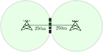
The performances of the developed algorithms are evaluated in a quasistatic frequency flat Rayleigh fading channel model. We model a scenario with adjacent cells, where all the users are between the two BSs to account for the most severe inter-cell interference situation, as illustrated in Fig. 2. In all the other figures except 10 and 11, we set the distance from the BSs to all the users to meters ( is the cell radius), and randomly assign them to multicasting groups of equal size. This models a scenario where the groups are very close to each other and all of the users have strong average interference. In Figures 10 and 11, where the methods are compared with existing schemes, we consider more typical scenarios where the users are randomly dropped between the cells so that the interference profiles between the users are different. The path loss is calculated as dB, where is the distance from BS to user . Each of the BSs serves equal number of randomly assigned user groups with users per group, i.e., the total number of users in the network is . We assume a bandwidth of 20 MHz and noise power is set to dBW. The antenna specific maximum power constraints are assumed to be equal for all the antennas over the whole bandwidth. The fixed simulation parameters are summarized in Table I while the other parameters are given in the figures.
| Parameters | Value |
|---|---|
| Path loss | [dB] |
| Cell radius | |
| Active RF chain-specific power | 0.4 W |
| Static power consumption | 4.5 W |
| Per-user power consumption | 0.1 W |
| Power amplifier efficiency | 0.35 |
| Maximum antenna-specific power | 1 W |
| Number of BSs | 2 |
| Number of groups per cell | |
| Number of users per group | |
| Number of Tx antennas | |
| Signal bandwidth | 20 MHz |
| Noise power | -125 dBW |
| 0.001 |
VI-A Algorithm performance
Fig. 3 illustrates the average convergence of the relaxed problem (i.e., phase 1) and the achieved EE (after phase 2) for Alg. 1 and Alg. 2. First in Fig. 3(a), we have run Alg. 1 with and . The same initial points have been used for both values of . We can see that the convergence speed in phase 1 is fast in the considered setting for both cases. However, we observe that they converge to different solutions. Specifically, the objective value of the relaxed problem (phase 1) after convergence is higher for , but the achieved EE (after phase 2) is worse than with . This is because with , more antenna selection variables are non-Boolean after convergence, which results in a worse antenna selection result. Another observation is that with (which achieves better energy efficiency), the objective value returned by the relaxed problem and the achieved EE are very close to each other. This means that the solution of the relaxed problem is already very close to Boolean. The better solution is achieved with only slightly decreased convergence speed of the relaxed problem. The examples demonstrate the effectiveness of the proposed formulation. The impact of on the average EE is studied in the next experiment. Fig. 3(b) then illustrates the convergence of Alg. 2 for different relaxations. We can observe that both smoothing functions provide fast convergence. Note that the methods converge to different objective values, because the curves show the convergence of phase 1. It is observed that compared to Alg. 1, the relaxation is very loose, but it still results in the same average EE after phase 2.


Fig. 4 illustrates the effect of on the average energy efficiency with different simulation parameters. We also illustrate the performance of the simplified algorithm (Alg. 1 ’simple’), where the beamformers achieved from the relaxed problem (i.e., step 7 is ignored in Alg. 1) are used for transmission. We can see that the choice of affects the achieved energy efficiency, and the choice of the best depends on the system parameters. In these cases, gives the best performance. More importantly, the choice of significantly affects the performance of the simple method, implying that it is enough to use the beamformers and antennas based on the relaxed problem for transmission. This reduces the computational load because step 7 can be ignored. The fact that the performance of the simple method is very close to the original method means that the solution of the relaxed method is very close to Boolean with the correct choice of . We also observe a saturation effect for implying that there exists a trade-off between the tightness of the continuous relaxation and the loss of optimality with the proposed algorithm.
Fig. 5 demonstrates the effect of penalty parameter on the average energy efficiency of Alg. 2 when using different smoothing functions to approximate . First, we observe that the convex relaxation (25) is not efficient in promoting sparsity because very high penalty parameter is required to yield the best energy efficiency. The performance is also highly dependent on the choice of , making it difficult to estimate good . Moreover, the achieved performance is still inferior to the other schemes, motivating the use of non-convex relaxations. We can see that all the non-convex relaxations result in approximately the same performance with the correct choice of . Also, a good performance is achieved even for , implying that the methods are efficient in promoting sparsity. It is observed that the relaxation (28b) is the best option in promoting sparsity with very small values of .
Fig. 6 shows the average EE versus the number of antennas per BS. First, we see that EE starts to decrease without antenna selection when . On the other hand, significant gains are achieved with the proposed algorithms and the gains naturally increase with the number of antennas. We can see that the simplified version of Alg. 1 is very close to the original method even when the number of antennas is large, which again motivates the effectiveness of the proposed formulation. On the other hand, as already observed in Fig. 6, Alg. 2 with (25) gives clearly worse performance than the other JBAS schemes do. However, Alg. 2 with (28a) and (28b) give the performance very close to Alg. 1, although slightly worse when the number of antennas is small. The reason for this is the fixed penalty parameter, which is now optimized for the larger number of antennas, resulting in too sparse a solution with smaller numbers of antennas. This is further investigated in Fig. 8. The reason why (25) is clearly worse is that it approximates by a pretty flat function, which is not very close to . As it is generally known, the convex approximations (like the -norm approximation) are easier to solve, but not efficient in promoting sparsity. The non-convex ones are far better in this regard, since they approximate by a tighter function which has a shape closer to . Thus, the nonconvex approximation is simply a better approximation of , resulting in an improved performance.
Fig. 7 illustrates the transmit powers versus with Alg. 1 and a method without antenna selection, with the same simulation parameters as those in Fig. 6. We can see that without antenna selection, it is energy-efficient to increase total transmit power when the number of antennas increases. This is achieved by decreasing the average transmit power per antenna. However, with JBAS, both the total transmit power and transmit power per antenna decrease when increases in the considered setting, until it starts to saturate. The reason is that when the number of antennas grows large enough, increasing the number of antennas for a fixed number of users does not provide additional SE gain, i.e., we end up with choosing the same number of antennas on average. This saturation of the number of the active antennas can be observed in Fig. 8. Increasing the number of antennas enables reducing the per-antenna power, meaning that the power amplifiers for each antenna can be cheaper. It can be concluded that the EE gains of the JBAS compared to the method without antenna selection are achieved by switching off some of the antennas but using larger per-antenna transmit power.

Fig. 8 displays the average number of active antennas to maximize the energy efficiency versus with the same simulation parameters as those in Fig. 6. It is observed that the more antennas available, the more active antennas are chosen for energy-efficient transmission. This makes sense, because when there are more antennas, there is more spatial diversity. Thus, sum rate gains due to better beamforming overwhelm the increased power consumption of activating some antennas. Also, the optimal number of antennas saturates to a certain value when grows large, because when the number of antennas is large enough, increasing the number of antennas for a fixed number of users provides little SE gain. As can be seen, Alg. 2 with (25) switches off too many antennas when the number of available antennas is small, and, on the other hand, not enough when is large. This also explains the performance gap in Fig. 6. In this case, has been chosen to give the best result for , which is clearly too large, when is smaller. Although being a simple method, the optimal penalty parameter has to be carefully chosen. By looking at the performance of the other schemes, we can see that the average number of active antennas for the best energy efficiency saturates to 17–18 in the considered setting. It can be concluded that when the number of users is fixed, it is energy-efficient to use a relatively small number of active antennas if the number of available antennas is much larger than the number of users in the system.

Fig. 9 illustrates the convergence of the SOCP approximation algorithm presented in Appendix D. The examples are for two different channel realizations and the same initial beamformers have been used for both algorithms. We can see that there is no significant difference in the convergence speed between the methods.

VI-B Comparison to Other Schemes
Here the proposed method is compared with some existing methods in the literature. Now the users are assumed to have random locations between the two BSs, and the results are averaged over user locations and channel realizations. One benchmark method is the multiuser MISO JBAS scheme in [35], where the SCA with semidefinite programming formulation and the norm is used to solve the JBAS problem. This method can be straightforwardly extended to the multi-cell multiuser scenario. Basically this means that compared to our multigroup multicast transmission, each user is served by different stream, i.e., it uses resources times more inefficiently, but can use better user-specific beamformers. Similarly we also extend the method in [35] to multi-cell multigroup multicasting scheme, i.e., to solve exactly the same problem. The second method in comparison is the multi-cell single-group multicasting scheme in [17], where the user groups inside the same cell are served by the orthogonal resources, but the neighboring cells reuse the same resources similarly. We also use the multi-cell single-group multicasting scheme using our proposed JBAS method.
In Fig. 10, the EE is plotted for different numbers of antennas. First, it is observed that the proposed methods are significantly superior to all the other schemes. As expected, the extension of JBAS method in [35] provides the closest performance to the proposed schemes. However, its inferiority to Alg. 1 is in line with the results observed from Fig. 6 already, where Alg. 2 with convex approximation provides significantly worse performance than the other schemes. Note that the method in [35] uses convex -norm, and uses semidefinite relaxation to approximate the EE problem, and then use SCA for further approximation. Thus, its complexity is higher [36], because the semidefinite relaxation dramatically increases the problem size, and the approximation is not so accurate because rank-1 solutions cannot be guaranteed [19].
In Fig. 11, we then investigate the effect of imperfect CSI on the average performance of the methods. The imperfect CSI is modeled so that the BSs have knowledge of the noisy channel , where is the perfect channel and is zero-mean complex Gaussian noise with variance per element. It is observed that the performance degrades when the accuracy of the channel decreases, as expected. However, Alg. 1 still achieves clearly the best performance, and JBAS is still very useful for EE improvements. It is also interesting to note that the performance of single-group transmission mode becomes closer to multigroup mode when the accuracy decreases. The reason for this is that there is less interference due to orthogonal transmission inside the cell, which makes the interference due to imperfect channel less significant.


VI-C EE-SR Tradeoff
Fig. 12 plots the average EE-SR trade-off curve. The trade-off curve has been simulated by sweeping the parameter from 0 to 1 in ’Alg. 1, PWEE‘ and from 0 to 5 in Alg. 3. It is observed that a lot wider trade-off region is achieved with joint beamforming and antenna selection. It is also observed that both of the proposed algorithms give the same average performance.

Fig. 13 shows the average number of active antennas in the trade-off curve. More specifically, we can see the number of active antennas which gives certain energy efficiency. In the considered setting, activating all the antennas gives the worst energy efficiency (this is the point where the sum rate is maximized). On the other hand, the energy efficiency maximizing number of active antennas is approximately 18, which yields the minimum sum rate. From Figs. 12 and 13, we can find the following observation. Looking at the EE-maximizing point of the method without AS, the JBAS scheme can maintain the same average sum rate as the scheme without AS, with more than 25% increase in the EE. This gain is achieved by switching off approximately half of the RF chains.

VII Conclusions
This paper has studied energy-efficient multi-cell multigroup coordinated joint beamforming and antenna selection with antenna-specific maximum power constraints and user-specific QoS constraints. Two different approaches based on mixed-Boolean programming and sparsity were proposed to solve this challenging problem. The resulting mixed-Boolean nonconvex optimization problem was tackled by a continuous relaxation and the successive convex approximation, where the antennas for which continuous antenna selection variables converge to zero are switched off. Different convex and non-convex approximations were proposed to solve the problem with sparsity-based formulation. We have also considered the trade-off between energy efficiency and sum rate by proposing two approaches to solve the problem. The numerical results have illustrated that both the continuous relaxation of mixed-Boolean program and the sparsity-based approaches provide very good performance for the considered problems. Moreover, the proposed methods can significantly improve energy efficiency over the method without antenna selection by switching off a portion of the antennas but using larger per-antenna transmit power. It is also observed that joint beamforming and antenna selection can be used to achieve wider energy efficiency and sum rate trade-off curve. It was also observed that when the number of users is fixed, it is energy-efficient to use a relatively small number of active antennas if the number of available antennas is significantly larger than the number of users in the system. Moreover, increasing the number of antennas significantly for a fixed number of users is not beneficial, because the energy-efficient number of active antennas starts to saturate. The EE-SR trade-off results also showed that the JBAS scheme can maintain the same average rate as the beamforming only method with more than 25% increase in the energy efficiency. This gain was achieved by switching off approximately half of the antennas. As a general conclusion, the energy-efficient beamforming strategy is not to use very low per-antenna power, but rather switch off many antennas and design energy-efficient beamformers for these and increase the per-antenna power.
References
- [1] R. Irmer, H. Droste, P. Marsch, M. Grieger, G. Fettweis, S. Brueck, H.-P. Mayer, L. Thiele, and V. Jungnickel, “Coordinated multipoint: Concepts, performance, and field trial results,” IEEE Commun. Mag., vol. 49, no. 2, pp. 102–111, Feb. 2011.
- [2] C. Xiong, G. Y. Li, S. Zhang, Y. Chen, and S. Xu, “Energy- and spectral-efficiency tradeoff in downlink OFDMA networks,” IEEE Trans. Wireless Commun., vol. 10, no. 11, pp. 3874–3886, Nov 2011.
- [3] C. He, B. Sheng, P. Zhu, X. You, and G. Y. Li, “Energy- and spectral-efficiency tradeoff for distributed antenna systems with proportional fairness,” IEEE J. Sel. Areas Commun., vol. 31, no. 5, pp. 894–902, May 2013.
- [4] F. Meshkati, H. V. Poor, and S. C. Schwartz, “Energy-efficient resource allocation in wireless networks,” IEEE Signal Process. Mag., vol. 24, no. 3, pp. 58–68, May 2007.
- [5] Y. Chen, S. Zhang, S. Xu, and G. Y. Li, “Fundamental trade-offs on green wireless networks,” IEEE Commun. Mag., vol. 49, no. 6, pp. 30–37, June 2011.
- [6] O. Tervo, L.-N. Tran, and M. Juntti, “Optimal energy-efficient transmit beamforming for multi-user MISO downlink,” IEEE Trans. Signal Process., vol. 63, no. 20, pp. 5574–5588, Oct. 2015.
- [7] E. Björnson, J. Hoydis, and L. Sanguinetti, “Massive MIMO networks: Spectral, energy, and hardware efficiency,” Foundations and Trends in Signal Processing, vol. 11, no. 3-4, pp. 154–655, 2017. [Online]. Available: http://dx.doi.org/10.1561/2000000093
- [8] E. Björnson, L. Sanguinetti, J. Hoydis, and M. Debbah, “Optimal design of energy-efficient multi-user MIMO systems: Is massive MIMO the answer?” IEEE Trans. Wireless Commun., vol. 14, no. 6, pp. 3059–3075, Jun. 2015.
- [9] O. Mehanna, N. Sidiropoulos, and G. Giannakis, “Joint multicast beamforming and antenna selection,” IEEE Trans. Signal Process., vol. 61, no. 10, pp. 2660–2674, May 2013.
- [10] M. A. Vazquez, A. Perez-Neira, D. Christopoulos, S. Chatzinotas, B. Ottersten, P. D. Arapoglou, A. Ginesi, and G. Tarocco, “Precoding in multibeam satellite communications: Present and future challenges,” IEEE Wireless Commun., vol. 23, no. 6, pp. 88–95, Dec 2016.
- [11] H. Pennanen, D. Christopoulos, S. Chatzinotas, and B. Ottersten, “Multicast multigroup precoding for frame-based multi-gateway satellite communications,” in Proc. Adv. Sat. Multimedia Systems Conf., Sep. 2016.
- [12] N. D. Sidiropoulos, T. N. Davidson, and L. Z.-Q., “Transmit beamforming for physical-layer multicasting,” IEEE Trans. Signal Process., vol. 54, no. 6, pp. 2239–2251, Jun. 2006.
- [13] E. Karipidis, N. Sidiropoulos, and Z.-Q. Luo, “Quality of service and max-min fair transmit beamforming to multiple cochannel multicast groups,” IEEE Trans. Signal Process., vol. 56, no. 3, pp. 1268–1279, Mar. 2008.
- [14] D. Christopoulos, S. Chatzinotas, and B. Ottersten, “Weighted fair multicast multigroup beamforming under per-antenna power constraints,” IEEE Trans. Signal Process., vol. 62, no. 19, pp. 5132–5142, Oct. 2014.
- [15] D. Christopoulos, S. Chatzinotas, and B. Ottersten, “Multicast multigroup precoding and user scheduling for frame-based satellite communications,” IEEE Trans. Wireless Commun., vol. 14, no. 9, pp. 4695–4707, Sep. 2015.
- [16] Z. Xiang, M. Tao, and X. Wang, “Coordinated multicast beamforming in multicell networks,” IEEE Trans. Wireless Commun., vol. 12, no. 1, pp. 12–21, Jan. 2013.
- [17] S. He, Y. Huang, S. Jin, and L. Yang, “Energy efficient coordinated beamforming design in multi-cell multicast networks,” IEEE Commun. Lett., vol. 19, no. 6, pp. 985–988, Jun. 2015.
- [18] O. Tervo, L. N. Tran, S. Chatzinotas, M. Juntti, and B. Ottersten, “Energy-efficient joint unicast and multicast beamforming with multi-antenna user terminals,” in Proc. IEEE Int. Workshop Signal Process. Adv. Wireless Commun., July 2017, pp. 1–5.
- [19] O. Tervo, H. Pennanen, D. Christopoulos, S. Chatzinotas, and B. Ottersten, “Distributed optimization for coordinated beamforming in multicell multigroup multicast systems: Power minimization and SINR balancing,” IEEE Trans. Signal Process., vol. 66, no. 1, pp. 171–185, Jan 2018.
- [20] M. Tao, E. Chen, H. Zhou, and W. Yu, “Content-centric sparse multicast beamforming for cache-enabled cloud RAN,” IEEE Trans. Wireless Commun., vol. 15, no. 9, pp. 6118–6131, Sep 2016.
- [21] J. Tang, D. K. C. So, E. Alsusa, K. A. Hamdi, and A. Shojaeifard, “On the energy efficiency-spectral efficiency tradeoff in MIMO-OFDMA broadcast channels,” IEEE Trans. Veh. Technol., vol. 65, no. 7, pp. 5185–5199, Jul 2016.
- [22] O. Amin, E. Bedeer, M. H. Ahmed, and O. A. Dobre, “Energy efficiency-spectral efficiency tradeoff: A multiobjective optimization approach,” IEEE Trans. Veh. Technol., vol. 65, no. 4, pp. 1975–1981, Apr 2016.
- [23] J. Tang, D. K. C. So, E. Alsusa, and K. A. Hamdi, “Resource efficiency: A new paradigm on energy efficiency and spectral efficiency tradeoff,” IEEE Trans. Wireless Commun., vol. 13, no. 8, pp. 4656–4669, Aug 2014.
- [24] O. Günlük and J. Linderoth, “Perspective reformulations of mixed integer nonlinear programs with indicator variables,” Mathematical Programming, vol. 124, no. 1-2, pp. 183–205, 2010. [Online]. Available: http://dx.doi.org/10.1007/s10107-010-0360-z
- [25] P. Bonami, M. Kilinç, and J. Linderoth, “Algorithms and software for convex mixed integer nonlinear programs,” in Mixed Integer Nonlinear Programming, ser. The IMA Volumes in Mathematics and its Applications, J. Lee and S. Leyffer, Eds. Springer New York, 2012, vol. 154, pp. 1–39. [Online]. Available: http://dx.doi.org/10.1007/978-1-4614-1927-3_1
- [26] Y. Cheng, M. Pesavento, and A. Philipp, “Joint network optimization and downlink beamforming for comp transmissions using mixed integer conic programming,” IEEE Trans. Signal Process., vol. 61, no. 16, pp. 3972–3987, Aug 2013.
- [27] O. Tervo, A. Tölli, M. Juntti, and L. N. Tran, “Energy-efficient beam coordination strategies with rate-dependent processing power,” IEEE Trans. Signal Process., vol. 65, no. 22, pp. 6097–6112, Nov 2017.
- [28] G. Venkatraman, A. Tölli, M. Juntti, and L. N. Tran, “Traffic aware resource allocation schemes for multi-cell MIMO-OFDM systems,” IEEE Trans. Signal Process., vol. 64, no. 11, pp. 2730–2745, Jun. 2016.
- [29] S. Boyd and L. Vandenberghe, Convex Optimization. Cambridge University Press, 2004.
- [30] A. Beck, A. Ben-Tal, and L. Tetruashvili, “A sequential parametric convex approximation method with applications to nonconvex truss topology design problems,” Journal of Global Optimization, vol. 47, no. 1, pp. 29–51, 2010.
- [31] S. Schaible, “Fractional Programming. I, Duality,” Management Science, vol. 22, no. 8, pp. 858–867, 1976.
- [32] Q.-D. Vu, M. Juntti, E.-K. Hong, and L.-N. Tran, “Conic Quadratic Formulations for Wireless Communications Design,” ArXiv e-prints, Oct. 2016.
- [33] F. R. Bach, R. Jenatton, J. Mairal, and G. Obozinski, “Optimization with sparsity-inducing penalties,” Foundations and Trends in Machine Learning, vol. 4, no. 1, pp. 1–106, 2012.
- [34] P. Ngatchou, A. Zarei, and A. El-Sharkawi, “Pareto multi objective optimization,” in Proc. Int. Conf. Intelligent Systems Application to Power Systems, Nov 2005, pp. 84–91.
- [35] S. He, Y. Huang, J. Wang, L. Yang, and W. Hong, “Joint antenna selection and energy-efficient beamforming design,” IEEE Signal Process. Lett., vol. 23, no. 9, pp. 1165–1169, Sept 2016.
- [36] A. Ben-Tal and A. Nemirovski, Lectures on Modern Convex Optimization. Society for Industrial and Applied Mathematics, 2001. [Online]. Available: https://epubs.siam.org/doi/abs/10.1137/1.9780898718829
- [37] J. Papandriopoulos and J. S. Evans, “SCALE: A low-complexity distributed protocol for spectrum balancing in multiuser DSL networks,” IEEE Trans. Inf. Theory, vol. 55, no. 8, pp. 3711–3724, Aug 2009.
Appendix A Proof of Lemma 1
Let use first prove inequality (i). Assume is an optimal solution (for some ()) of the continuous relaxation of (7) (i.e., using ). Then, the denominator of the objective function (9a) at the optimal point is written as . Note that in this case the constraint may not be tight. On the other hand, assume that we then use , i.e., solve continuous relaxation of (9). Then, assume that (i.e., optimal solution of the relaxation of (7)) is its optimal solution. The power consumption can be written as . Now, assuming that would be the optimal solution, according to the constraint , we can always decrease compared to the original formulation to make the denominator smaller (unless ) such that . This also contradicts the fact that are optimal for the continuous relaxation of (9), and implies that the optimal objective value has to be smaller for the continuous relaxation of (9). Thus, because , it has to hold that . This yields , which again implies that . Similarly the proof for (ii) follows from the fact that , which implies that , i.e., and . The inequality in (iii) is simply because the optimal value with any continuous relaxation is larger than that of the Boolean formulation.
Appendix B Proof of Lemma 2
For proving the lemma, we show that constraints (13b) and (13d) are active at the optimality by contradiction. Let be an optimal solution of (13) with optimal value and suppose that (13b) is not active at the optimum for the worst user in some group, i.e., for some . Then we can scale down the transmit power for user group and achieve a new beamformer such that for while keeping the others unchanged, i.e for all . In this way, we then achieve for all since interference power at all the other users has reduced. Thus, to improve the objective, we could then increase for all until . In addition, we then also have (because we have reduced the transmit power for group ), which means that we could reduce either or to make the denominator of (13a) smaller. This implies that we have . Consequently, this contradicts the fact that is the optimal solution, completing the proof.
Appendix C Convergence Analysis of the Iterative Algorithm for Solving (16)
Here we show that the the objective function (19a) converges monotonically, i.e., improves at every iteration and is bounded above. Let be the optimal objective obtained at iteration of the proposed SCA-based algorithm, i.e., is the optimal objective of (19). We will show that , i.e., the objective sequence is monotonically increasing. To this end we prove that the solution obtained at iteration is also feasible to the problem considered at iteration .
Let us first focus on the constraint (19b) and denote by , , and the optimal values of , and , respectively at iteration . It immediately holds that
| (40) |
where the first inequality is obvious and the second one is due to (18). At iteration (19b) becomes
| (41) |
Substituting , , and into the above inequality results in
| (42) |
which is true due to (40). That is, , , and are feasible to (19b) at iteration . Similarly, the same result can also proved for (19c). Consequently, we can conclude that the solution obtained at iteration is also feasible to the convex program considered at iteration , and thus .
The sequence is bounded from above due to the limited transmit power, and thus it is convergent. It is difficult to comment on the convergence of the iterates (i.e., optimization variables) generated by the algorithm as the objective in (19a) is not strongly concave. A possible way to achieve the convergence of the iterates is to introduce a sufficiently large proximal term in the objective of (19a). However, this method is quite involved and, thus, not considered in this paper.
Appendix D Iterative SOCP Method to Solve (11)
The solution proposed in Section III-B1 requires solving a generic non-linear concave-convex fractional program (19) in each iteration. This can be equivalently transformed to a generic non-linear convex program (20) which is still difficult to solve efficiently due to the exponential cone in constraint (20i). Here we aim at finding a more efficient formulation. Specifically, all the other constraints in (19) admit the second-order cone form except the log-term in (13d). To avoid the use of log-function, we need to find a concave lower bound for to fulfill the conditions of the SCA. To this end, we use the following lower bound approximation for the concave log-function [37]
| (43) |
which is tight at , when the coefficients are chosen as
| (44) |
As a result, we follow the description of Algorithm 1 but solve the following SOCP at step 2
| (45a) | |||||
| (45b) | |||||
| (45c) | |||||
| (45d) | |||||
| (45e) | |||||
| (45f) | |||||
| (45g) | |||||
| (45h) | |||||
| (45i) | |||||
In the above problem, all the other constraints are linear except (45c) and (45h) which can be expressed as , where is some vector, and are scalars. These constraints are equivalently written in the SOC form as
| (46) |
More specifically, let us first consider (45c) and denote as the fixed coefficients in . Then, we can write it equivalently as . Thus, according to (46), we can write , and substituting these to (46) is equivalent to (45c). On the other hand, (45h) is readily in a form , where . In this case, , where is a scalar.
Appendix E Complexity Analysis
Here we provide a complexity comparison based on the worst-case analysis presented in [36]. The worst-case complexity of Alg. 1 depends on the number of variables and can be upper bounded as
| (47) | |||
| (48) |
where and are the number of performed iterations in the relaxed problem (steps 1-5) and lower-dimensional problem for fixed antenna set (steps 6-7), respectively, is the number of antennas selected for transmission, is the total number of users, and is the total number of groups. Taking the dominant terms, it can be approximated as
| (49) |
where the dominant term depends on the relation between and . Note that Alg. 1 ‘simple’ reduces the complexity compared to Alg. 1 so that the second term in the above equation is ignored. The complexity reduction depends on the number of iterations and complexity to solve the lower-dimensional problem in steps 6-7 of Alg. 1. We note that the above upper bound for the complexity is quite conservative as a solution can be found much faster in reality. On the other hand, the worst-case complexity of solving the SOCP in Appendix D can be written as
| (50) | |||
| (51) |
where is the number of iterations. This algorithm provides a sharp complexity reduction compared to the generic formulation.