Benefit of Self-Stabilizing Protocols in Eventually Consistent Key-Value Stores: A Case Study
Abstract.
In this paper, we focus on the implementation of distributed programs in using a key-value store where the state of the nodes is stored in a replicated and partitioned data store to improve performance and reliability. Applications of such algorithms occur in weather monitoring, social media, etc. We argue that these applications should be designed to be stabilizing so that they recover from an arbitrary state to a legitimate state. Specifically, if we use a stabilizing algorithm then we can work with more efficient implementations that provide eventual consistency rather than sequential consistency where the data store behaves as if there is just one copy of the data. We find that, although the use of eventual consistency results in consistency violation faults () where some node executes its action incorrectly because it relies on an older version of the data, the overall performance of the resulting protocol is better. We use experimental analysis to evaluate the expected improvement. We also identify other variations of stabilization that can provide additional guarantees in the presence of eventual consistency. Finally, we note that if the underlying algorithm is not stabilizing, even a single may cause the algorithm to fail completely, thereby making it impossible to benefit from this approach.
Keywords:
Fault tolerance, Self-stabilization, Key-value stores1. Introduction
A typical distributed system protocol (Coulouris et al., 2011; Ghosh, 2014) in a shared memory model views the system in terms of a graph with the given set of nodes (processes) and edges (links) between them. Furthermore, the protocol consists of a set of actions for each node. An action at a node, say , reads the state of (one or more of) its neighbors and updates its own state. In other words, each node is thought of as an active entity associated with some computing power as well as an ability to communicate.
Examples of such applications include spanning trees (Arora and Gouda, 1994; Huang and Chen, 1992) leader election (Altisen et al., 2017; Datta et al., 2011), matching (Inoue et al., 2017; Datta et al., 2015), dominating set (Kobayashi et al., 2017; Kakugawa and Masuzawa, 2006), independent set (Ikeda et al., 2002; Hedetniemi et al., 2012), clustering (Datta et al., 2016; Datta et al., 2010; Caron et al., 2009). In these applications, each node runs a protocol that consists of some actions that detect and correct some variables according to the given specification. Some examples of these variables are parent variable in a spanning tree protocol, a leader variable in a leader election protocol, etc.
In recent literature, this model is extended to scenarios where the nodes are themselves viewed as passive entities. As an example, consider the problem of matching in a graph with a large number of nodes. Such a problem arises in computations associated with social media, weather monitoring. In these systems, instead of treating each node as an active entity that reads the state of its neighbors to update its own state, we view them as passive entities. Thus, the states of different nodes are stored in some database (e.g., key-value store). Furthermore, the state(s) of the nodes is replicated for resilience and efficiency. Additionally, we introduce clients that are assigned a set of nodes in the graph. The job of the clients is to execute the actions associated with the given set of nodes. In other words, each client is assigned a set of nodes (either statically or dynamically) to operate on. If client is assigned node , client reads the state of and its neighbors from the common storage. Then, it updates the state of based on the action(s) of .
This new model, denoted as the passive-node model, provides several advantages. For one, it is much easier to deal with graphs which contain thousands or millions of nodes. By contrast, creating these many processes running in parallel in the active model is not feasible. It allows us to control the level of concurrency by choosing the number of clients. It allows us to improve scalability via replication.
In the composite atomicity shared memory model, it is assumed that each action of the program is executed atomically. In the active-node model, where each node is independently reading the state(s) of its neighbor(s), extra work is needed (Dolev, 2000; Ghosh, 2014) to ensure the resulting program behaves correctly in read-write model or message passing model. One way to achieve the required level of atomicity is to utilize local mutual exclusion (Beauquier et al., 2000; Nesterenko and Arora, 2002; Kakugawa and Yamashita, 2002) so that when one node is executing its actions, its neighbors are not. The same approach can be used in the new passive-node model as well. However, this introduces some opportunities as well as challenges. One advantage is that since the set of clients is working on only a small subset of nodes (among the thousands or millions of total nodes) at a given time, it is likely that the conflict among them is reduced. However, a key disadvantage is that the underlying data store may not provide sequential consistency. Sequential consistency allows one to view replicated data store as if there was just one copy, it guarantees each client is seeing the latest state of the data store. If the data store only provides eventual consistency, the client may be reading an older version of the data and not be aware of it.
In general, to translate a given protocol into the passive-node model, we must provide local mutual exclusion and sequential consistency. This is due to the fact that without sequential consistency, it is possible that when a client updates the state of node , no other client updates the state of the neighbor of . However, the states read by this client are stale because the underlying data store is not providing the latest state of those neighbors. Thus, if sequential consistency is not provided by the underlying data store, even if local mutual exclusion is provided, an action of node may not correspond to a permitted execution in the shared memory model.
Now consider an execution of a shared memory program (such as those for matching, spanning tree, ) that is being run in a passive-node model where the states of the nodes are stored in a distributed data store and a set of clients update those states based on the given program. Also, assume that each client utilizes local mutual exclusion to ensure that when it is updating the state of one node, other clients are not modifying the states of that node’s neighbors. In such an execution, as long as sequential consistency happens to be satisfied (e.g., by sheer luck even though the underlying consistency model is weaker), the execution would be the execution of the abstract program in shared memory model. However, if the computation includes even a single execution of an action that relies on an inconsistent state of one neighbor then subsequent computation may not correspond to a valid computation of the given abstract program.
To deal with this problem, the program needs to (1) disallow a client to update the state of a node when sequential consistency is likely to be violated, or (2) detect if sequential consistency is violated and rollback, or (3) permit for a possible inconsistent execution and treat it as a fault. (We note that the third option also permits the possibility that the property of local mutual exclusion is violated during the execution as we can treat it as a fault as well. We consider this in our analysis in Section 7.)
Of these, the first option increases the cost substantially as we would pay the penalty for providing sequential consistency. The second option requires one to create a monitor and some type of checkpointing mechanism to rollback the state of the given system. Clearly, both options have the potential to result in excessive overhead. This suggests that the third option should be explored. However, in general, if a node executes its action(s) incorrectly, the result may be unpredictable and, hence, its effect on the correctness of the given program cannot be determined.
In this paper, we evaluate whether using a self-stabilizing algorithm can permit us to use the third option in terms of providing desirable program behavior as well as in terms of performance. A self-stabilizing program (Dijkstra, 1974) guarantees that starting from an arbitrary state, in finite time, the program recovers to a legitimate state. Thus, if a node executes its action incorrectly, we can simply treat it as a perturbation. And, by its nature, a self-stabilizing program is designed to deal with state perturbation.
With this observation, we consider the execution of a self-stabilizing program as a sequence, where is an initial (arbitrary) state. Furthermore , is either a valid or invalid execution of some action in the program. For the sake of discussion, let be an invalid transition of some node. The resulting state, is still a state of the program. Given that the program is stabilizing, even the computation from is guaranteed to converge to a legitimate state.
In this context, the natural question is: will the invalid execution of some node cause stabilization property to be lost? In the worst case, if the number of such perturbations is frequent, then the convergence property would be violated. Also, it is possible that the perturbation causes the program to be in a state that is worse than in terms of the time required for convergence. In general, since the perturbation is, by design, random/non-deliberate (since it depends upon the race condition where the data store happens to provide the wrong data that allows some client to execute an action incorrectly) and rare (since it requires the affected node to execute exactly at the wrong time and clients are operating only on a small subset of nodes at a time), we expect that the perturbation is likely to have (on average) a small impact on the convergence. The goal of this paper is to evaluate this intuition to validate the benefit of designing a self-stabilizing program in eventual consistent data stores. In this paper, we validate this intuition. Specifically,
- •
We introduce the notion of consistency violation faults () that may occur due to the use of eventual consistency.
- •
With experimental analysis, we show that even though execution in eventual consistency suffers from , it outperforms significantly when compared with the use of sequential consistency. This observation remains valid even if the program was initialized to a proper initial state.
- •
We argue that some stronger versions of stabilization would be even more valuable in providing additional guarantees about the protocols that use eventual consistency.
We note that the benefit of using eventual consistency while tolerating is feasible only if the underlying algorithm is stabilizing. Without stabilization, it is possible that even a single may cause the protocol to fail to a state from where it cannot recover. Such a situation does not arise in stabilization since is weaker than an arbitrary transient fault that is tolerated by a stabilizing program. From this, we argue that designing protocols to be stabilizing is especially beneficial in the context of graph-based applications that use replicated, partitioned data store.
2. System Model/Architecture
In this section, we define some important concepts to be used in this paper. Section 2.1 describes the model of the distributed programs used in this work. We discuss how these programs are modeled in the traditional active-node model in Section 2.2. Subsequently, Section 2.3 describes the computation of the system where nodes in the distributed system are thought to be passive and a set of clients operate on them. We discuss the similarity between these models in Section 2.4. (The differences in these models is discussed in Section 4.) Finally, we define the notion of stabilization in Section 2.5.
2.1. Distributed Programs
A program consists of a set of nodes and a set of edges . We assume that for any node , edge is included in . Each node, say , in is associated with a set of variables . The set of variables of program , denoted by , is obtained by the union of the variables of nodes in . A state of is obtained by assigning each variable in a value from its domain. State space of , denoted by , is the set of all possible states of .
Each node in program is also associated with a set of actions, say . An action in is of the form , where is a predicate involving and updates one or more variables in . We say that an action (of the form ) is enabled in state iff evaluates to true in state . The transitions of action (of the form ) are given by , is true in and is obtained by execution in state }. Finally, transitions of node (respectively, program ) is the union of the transitions of its actions (respectively, its nodes). We use and to denote transitions corresponding to action , node and program respectively.
2.2. Traditional/Active-Node Model
Computation. In the traditional/active-node model, the computation program is of the form where
- •
, is a state of ,
- •
is a transition of or
( and no action of is enabled in state ), and - •
If some action of (of the form ) is continuously enabled (i.e., there exists such that is true in every state in the sequence after ) then is eventually executed (i.e., for some , corresponds to execution of .)
The above computation model corresponds to the centralized daemon with interleaving semantics where in each step, only one node can execute at a given time. This can be implemented in read-write atomicity or message passing model by solutions such as local mutual exclusion, dining philosophers, etc. The resulting computation guarantees that two neighboring nodes do not execute simultaneously. In turn, the resulting computation is realizable in the original model. (Our observations/results are also applicable to other models. We discuss this in Section 7.)
2.3. Passive-Node Model
The structure of the program (in terms of its nodes and actions) remains the same in the passive-node model. The only difference is in terms of the execution model. Specifically, the system consists of a replicated and partitioned key-value store that captures the current state of . In other words, the state of is stored in terms of pairs of the form , where is a key (i.e., the name of the variable and node ID) and is the corresponding value. Additionally, the system contains a set of clients. The role of the clients is to execute the actions of one or more nodes assigned to them (either statically or dynamically).
In an ideal environment, the execution of the program is performed as follows: Let node be assigned to client . Then, reads the values of the variables of and its neighbors. If it finds that some action of is enabled, it updates the key-value store with the new values for the variables of . Similar to active-node model, it is required that actions of multiple nodes can be serialized.
Computation. The notion of computation in passive-node model is identical to that of active-node model from Section 2.2; the only difference is the introduction of clients in the passive-node model. Furthermore, by requiring the clients to execute actions of each node infinitely often, it guarantees the fairness assumed in the definition of computation in Section 2.2.
2.4. Similarity between Active-Node and Passive-Node Model
The active-node model relies on two requirements (1) each node is given a fair chance to execute, and (2) execution corresponds to a sequence of atomic executions of actions of some nodes. The first requirement is satisfied as long as each client considers every node infinitely often; if some action is enabled continuously, eventually a client would execute that action. The second requirement, atomicity of individual actions, is satisfied if (1) clients enforce local mutual exclusion among nodes, i.e., if we ensure that clients and do not operate simultaneously on nodes and that are neighbors of each other and (2) when a client reads the value of any variable (key), it obtains the most recent version of that variable (key).
Of these, the requirement for mutual exclusion was necessary even in the active-node model. The ability to read the most recent value was inevitable in the active-node model. Specifically, if node reads the values of its neighbors after it had acquired the local mutual exclusion, it was guaranteed to read the latest state of its neighbors. In the passive-node model, this requirement would be satisfied if we have only one data store (i.e., no replication) that maintains the data associated with all nodes or the replicated data store appears as a single copy. In particular, if the replicated data store provides a strong consistency such as sequential consistency, this property is satisfied. However, if it provides a weaker consistency such as eventual consistency, this property may be violated. We discuss the details of this sequential/eventual consistency, next.
2.5. Stabilization
In this section, we recall the definition of stabilization from (Dijkstra, 1974). This definition relies on the notion of computation. As discussed in Section 2.2 and 2.3, computations can be defined in both active-node model and passive-node model. We use this notion of computation in defining stabilization.
Stabilization. Let be a program. Let be a subset of state space of . We say that is stabilizing with state predicate iff
- Closure::
-
If program executes a transition in a state in then the resulting state is in , i.e., for any transition , , and
- Convergence::
-
Any computation of eventually reaches a state in , i.e., for any that is a computation of , there exists such that .
In our context, we use to capture the predicate to which program recovers so that the subsequent computation satisfies the specification. We use the term invariant of to denote this predicate. In our initial discussion, we focus only on the convergence property. Hence, we focus on silent stabilization which requires that upon reaching the invariant, the program terminates, i.e., it has no further actions that it can execute. Thus, we have
Silent Stabilization. Let be a program. Let be a subset of state space of . We say that is silent stabilizing with state predicate iff
- Closure::
-
Program has no transitions that can execute in , i.e., for any , for any state , and
- Convergence::
-
Any computation of eventually reaches a state in , i.e., for any that is a computation of , there exists such that .
Our initial discussion focuses on silent stabilization. We discuss generalized stabilization in Section 7.
3. Distributed Key-Value Store
In the passive-node model, the state of the given program is saved in a key-value store. We use Voldemort (Vol, [n. d.]) in this paper. However, our approach is equally applicable to other key-value stores such as those in (Lakshman and Malik, 2010; Olson et al., 1999; Dyn, [n. d.]). In this section, we describe the important properties of the key-value store relevant to the passive-node model.
In a key-value store, clients share a common data stored at replicated and partitioned servers. The data consists of one or more tables where each entry in the table is of the form where is the key and is the corresponding value. In our experiments, keys correspond to the unique names of the program variables and values correspond to the current value assignment.
The data at the store is managed with two operations: PUT and GET. PUT(key=,value=) tries to update the value of key . If the data store does the not have key , then it will create a new entry and save it. In case the data store already has key then data store uses vector clocks (Fidge, 1987; Mattern, 1989) to determine whether the new value should be stored. In case of concurrent updates, multiple values are stored. Subsequently, the server sends an acknowledgment to the client. Operation GET() returns all concurrent versions associated with key that are available at the store. When multiple versions for a key are returned, the client resolves them by some approach such as last-write-win.
For efficiency, accessibility, and fault tolerance reasons, tables are divided into smaller partitions, and each partition is replicated at multiple servers. We assume each replica stores all partitions.
One of the most popular key-value stores is Amazon’s Dynamo. In our experiments, we use Voldemort, an open-source equivalence of Dynamo developed by LinkedIn. Voldemort uses active replication, i.e. the Voldemort client-library at the client side is responsible for replication. The client uses GET/PUT to access the data. These calls into client-library mask the details of replication, failure handling, and resolution of multiple versions from the client application.
When a client-library establishes a connection to the data store, it receives the configuration meta-data from the server which includes: the list of servers and their addresses, replication factor (N), required reads (R), required writes (W).
When the client-library receives a PUT (or GET) request from the application, it sends PUT (or GET) requests to N servers and waits for a predetermined amount of time (e.g. 500 milliseconds). If at least W (or R) acknowledgement (or responses) are received before the timeout, the operation is successful. The client-library may process the results (e.g. resolve the conflicts when multiple versions are received) before returning the final result to the application. If less than W (or R) replies are received after a threshold number of attempts, the operation is unsuccessful and the client-library returns an exception to the application.
We chose Voldemort for our experiments because it provides a convenient approach to deploy both sequential and eventual consistency. In particular, if and then the consistency level is sequential. Otherwise, it provides eventual consistency. This allows us to perform the experiments for sequential and eventual consistency in the same code base by simply changing the values of R and W. We denote these variations with notation RaWb. For example, R2W1 denotes that and .
4. Consistency Violation Faults ()
As discussed above, in a replicated system, the state of each node is maintained at each replica. In particular, for each variable of node , each replica maintains the value of as a key-value pair. For the sake of discussion, we assume that there are three replicas and the value of in these replicas are and . We define the (abstract) value of to be , where is some resolution function. Intuitively, function will provide the latest value of . While the actual function is irrelevant for our purpose, we only assume that returns either , or .
Now, consider the computation of a program in the passive-node model. If there was only one replica in the system, anytime the client read the value of some variable, say , it will read the corresponding abstract value of . Furthermore, when a client writes the value of , it will change the abstract value of . However, with eventual consistency, this assumption may be violated.
Consistency Violating Faults (). With this observation, we can now view the computation of the given program as a sequence such that most transitions in this sequence correspond to the transitions of . However, some transitions correspond to the scenario where some node reads an inconsistent value for some variable and updates one or more variables of . By design, the incorrect execution corresponds to changing one or more variables of one node. Thus, the effect of incorrect execution (denoted as concurrency violating faults ()) is a subset of and , differ only in the variables of some node of
Remark. Whenever is clear from the context, we use instead of .
Computation in the presence of . With the definition of , we can see that computation of program in a given replicated passive-node model is of the form where
- •
, is a state of ,
- •
or
and no action of is enabled in state , and - •
If some action of (of the form ) is continuously enabled (i.e., there exists such that is true in every state in the sequence after ) then is eventually executed (i.e., for some , corresponds to execution of .)
Expected Properties of . If we run a distributed program in the passive-node model – with a large number of nodes but relatively fewer clients– with an eventually consistent key-value store then its execution would be a computation in the presence of . We expect the following observations for :
- •
A single only affects one node.
- •
is expected to be rare; to be affected by , we need to have one client, say , operating on node and another client, say , operating on neighboring node where state of is updated on one replica but reads it from another replica.
- •
By design, is not deliberate. While some specific single perturbation in a stabilizing program can significantly affect the convergence property, the probability that would result in that specific perturbation is small.
- •
Between two transitions, the program is likely to execute several valid transitions.
- •
Let be a transition of node . One type of occurs when reading an inconsistent value of some variable results in to evaluate to false. In this case, the effect of results in stuttering of the same state. In this case, the recovery of program is unaffected.
Now, consider the execution of a program from its arbitrary state, say , in the presence of . In this computation, is attempting to change its state so that it reaches its invariant. A can perturb this recovery. However, from the above discussion, the effect of on recovery time is expected to be small. By contrast, the cost of eliminating (i.e., utilize sequential consistency) is expected to slow down the execution of program . In this paper, we evaluate this hypothesis to determine if permitting occasional with eventual consistency is likely to provide us with a better recovery time that eliminating with sequential consistency.
5. Experimental Evaluation of Benefits of Stabilization in Key-Value Stores
As discussed in Section 4, if we run a stabilizing program with eventually consistent key-value store, it may suffer from consistency violation faults (). In this section, we evaluate the hypothesis that even if the convergence is perturbed by , using eventual consistency would improve the overall convergence time. We use the algorithm by Manne et al. (Manne et al., 2009) for maximum matching to perform the evaluation. We note that our analysis depends upon the occurrence of and, hence, it is equally applicable to other stabilizing algorithms as well.
5.1. Experiment Setup
We conduct the experiment in a local network with 9 commodity PCs (Intel Core i5, 4GB RAM). 3 PCs are reserved for the 3 key-value store servers and the clients are evenly distributed among the remaining 6 PCs.
We conduct experiments with three initial configurations: no-match, random-match and perturbed-match. The no-match experiment initializes global state so that no node is matched with any other node, characterizing execution from a properly initialized state. The random-match experiment initializes each node so that match of node is either (not matched) or some node in the network. (Of course, in the initial state if is matched with it does not imply that is matched with .) The random-match corresponds to random initial state of the program. The perturbed-match experiment perturbs 10% of the nodes from an invariant state (i.e., a state where maximal matching has been achieved). We use the same set of initial states in each experiment. In other words, the same initial state is used to compare sequential consistency with eventual consistency. In our experiments, we use three replicas. As discussed in Section 3 for sequential consistency, we use R1W3 and R2W2 models whereas for eventual consistency, we use R1W1. We repeat each experiment 3 times and take an average.
We use a variation of the termination detection algorithm (Dijkstra et al., 1983) to detect when the system has reached a point where a maximal matching has been formed. However, for reasons of space, we omit the details of how this is achieved. We only note that the task of detecting termination does not affect the time required for performing the matching.
5.2. Experiment Results
We conduct five types of experiments to validate our hypothesis that permitting by utilizing stabilizing algorithms is beneficial compared with the use of sequential consistency and local mutual exclusion where are prevented. We conduct experiments to (1) validate this hypothesis, (2) improve performance further by improving efficiency where the occurrence of is increased, and (3) evaluate the effect of concurrency (i.e., increased number of clients), (4) evaluate the convergence pattern to compare the intermediate states of the program before convergence, and (5) validate the soundness of results in a realistic environment with Amazon AWS.
Experiment 1: Sequential vs Eventual Consistency. Our first set of experiments focuses on comparing eventual consistency with and sequential consistency. Recall that the latter does not suffer from as each client gets the latest state of every node. The results are shown in Table 1.
| Initial state | Consistency | Graph size (# nodes) | ||
| 5,000 | 10,000 | 20,000 | ||
| random-match | R1W1 | 180 | 399 | 851 |
| R2W2 | 305 | 637 | 1496 | |
| R1W3 | 234 | 497 | 1080 | |
| Speedup over R2W2 | 1.7 | 1.6 | 1.8 | |
| Speedup over R1W3 | 1.3 | 1.2 | 1.3 | |
| perturbed-match | R1W1 | 123 | 273 | 650 |
| R2W2 | 184 | 450 | 1136 | |
| R1W3 | 155 | 349 | 808 | |
| Speedup over R2W2 | 1.5 | 1.6 | 1.7 | |
| Speedup over R1W3 | 1.3 | 1.3 | 1.2 | |
| no-match | R1W1 | 119 | 273 | 563 |
| R2W2 | 200 | 445 | 976 | |
| R1W3 | 156 | 363 | 779 | |
| Speedup over R2W2 | 1.7 | 1.6 | 1.7 | |
| Speedup over R1W3 | 1.3 | 1.3 | 1.4 | |
We find that even with , the convergence time with eventual consistency is significantly lower. Specifically, for configuration no-match, random-match, and perturbed-match, the convergence speedup factor is 1.3 – 1.7, 1.2 – 1.8, and 1.2 – 1.7, respectively. Moreover, the benefit remains fairly constant as the number of nodes increases.
Experiment 2: Revisiting Local Mutual Exclusion. Recall that to ensure that the execution in the passive-node model is free from , we need to use sequential consistency and local mutual exclusion. Note that without local mutual exclusion, implementation of a protocol may suffer from inconsistencies. However, their effect is the same as .
From this observation, we first compare the convergence time for the program using local mutual exclusion and sequential consistency with the program using eventual consistency and no local mutual exclusion. The results are shown in Table 2.
| Initial state | Consistency | Graph size (# nodes) | ||
|---|---|---|---|---|
| 5,000 | 10,000 | 20,000 | ||
| random-match | R1W1-no-lme | 31 | 63 | 129 |
| R1W1-lme | 180 | 399 | 851 | |
| R2W2-lme | 305 | 637 | 1496 | |
| R1W3-lme | 234 | 497 | 1080 | |
| Speedup over R1W1-lme | 5.8 | 6.3 | 6.6 | |
| Speedup over R2W2-lme | 9.9 | 10.0 | 11.6 | |
| Speedup over R1W3-lme | 7.6 | 7.8 | 8.4 | |
| perturbed-match | R1W1-no-lme | 19 | 47 | 110 |
| R1W1-lme | 123 | 273 | 650 | |
| R2W2-lme | 184 | 450 | 1136 | |
| R1W3-lme | 155 | 349 | 808 | |
| Speedup over R1W1-lme | 6.6 | 5.8 | 5.9 | |
| Speedup over R2W2-lme | 9.8 | 9.5 | 10.3 | |
| Speedup over R1W3-lme | 8.3 | 7.4 | 7.3 | |
| no-match | R1W1-no-lme | 19 | 43 | 94 |
| R1W1-lme | 119 | 273 | 563 | |
| R2W2-lme | 200 | 445 | 976 | |
| R1W3-lme | 156 | 363 | 779 | |
| Speedup over R1W1-lme | 6.2 | 6.3 | 6.0 | |
| Speedup over R2W2-lme | 10.5 | 10.3 | 10.4 | |
| Speedup over R1W3-lme | 8.2 | 8.4 | 8.3 | |
From this table, we observe that even in the presence of increased due to unavailability of local mutual exclusion (lme), the time for convergence is significantly lower with eventual consistency. Specifically for configurations no-match, random-match, and perturbed-match, the convergence speedup factor of eventual consistency without lme over sequential consistency (with lme) is 8.2 – 10.5, 7.6 – 11.6, and 7.3 – 10.3, respectively.
Experiment 3: Effect of Increased Concurrency. A key advantage of passive-node model is that the level of concurrency can be managed. Specifically, we can increase the number of clients to increase the level of concurrency. To evaluate the effect of on increased level of concurrency, we conducted the setup for Experiment 3 with 15, 30, and 45 clients. The graph size is 10,000 nodes. The results are shown in Table 3. From this table, we observe that the benefit of tolerating s with eventual consistency remains (fairly) same as the concurrency level is increased.
| Consistency | Number of clients | ||
|---|---|---|---|
| 15 | 30 | 45 | |
| R1W1-no-lme | 63 | 52 | 71 |
| R1W1-lme | 399 | 407 | 500 |
| R2W2-lme | 637 | 638 | 812 |
| R1W3-lme | 497 | 416 | 548 |
| Speedup over R1W1-lme | 6.3 | 7.9 | 7.0 |
| Speedup over R2W2-lme | 10.0 | 12.3 | 11.4 |
| Speedup over R1W3-lme | 7.8 | 8.0 | 7.7 |
Experiment 4: Convergence pattern. General trend of convergence for both sequential and eventual consistency looks like a sigmoid shape as shown in Figure 1. It starts slowly when nodes try to find their matches by making, withdrawing, and accepting proposals. Once some matches are formed, the matching progress quickly since the number of matching options is reduced. At the end, the progress slows down, as it takes time for a dead node to determine that it will remain unmatched.
From this figure, we find that at any given time , the level of matching performed with eventual consistency is higher. In other words, the benefit of eventual consistency is not caused by the last few nodes that delay the completion of the matching algorithm.
Experiment 5: Experiments on Amazon AWS. To validate our results in a more realistic setting, we deploy similar experiments on a subset of the settings on Amazon AWS EC2 instances. The servers run on M5.xlarge instances (4 vCPUs, 16 GB RAM), the termination detector and the clients run on M5.large instances (2 vCPUs, 8 GB RAM). The instances are distributed in three different availability zones of a same region (Ohio, USA). As shown in Table 4 , the results in the AWS experiments have similar characteristics as those in the experiments deployed on local machines, except that it takes longer time to converge in the AWS experiments because of longer network latency. In fact, the benefit in Amazon AWS experiments is higher than the values observed in Experiment 1. This is due to the fact that latencies in Amazon AWS network are higher than in Experiment 1 where machines are on the same local network. In other words, increased latency is improving the benefit of eventual consistency with over sequential consistency.
| Initial state | Consistency | Graph size (# nodes) | ||
|---|---|---|---|---|
| 5,000 | 10,000 | 20,000 | ||
| random-match | R1W1-no-lme | 66 | 139 | 277 |
| R1W1-lme | 385 | 938 | 1629 | |
| R2W2-lme | 791 | 1666 | 3307 | |
| R1W3-lme | 548 | 1249 | 2426 | |
| Speedup over R1W1-lme | 5.8 | 6.8 | 5.9 | |
| Speedup over R2W2-lme | 12.0 | 12.0 | 11.9 | |
| Speedup over R1W3-lme | 8.3 | 9.0 | 8.7 | |
| perturbed-match | R1W1-no-lme | 48 | 114 | 238 |
| R1W1-lme | 250 | 582 | 1345 | |
| R2W2-lme | 531 | 1283 | 2262 | |
| R1W3-lme | 373 | 877 | 1902 | |
| Speedup over R1W1-lme | 5.2 | 5.1 | 5.7 | |
| Speedup over R2W2-lme | 11.1 | 11.2 | 9.5 | |
| Speedup over R1W3-lme | 7.8 | 7.7 | 8.0 | |
| no-match | R1W1-no-lme | 45 | 86 | 145 |
| R1W1-lme | 241 | 570 | 1154 | |
| R2W2-lme | 524 | 1099 | 2221 | |
| R1W3-lme | 396 | 817 | 1644 | |
| Speedup over R1W1-lme | 5.3 | 6.7 | 8.0 | |
| Speedup over R2W2-lme | 11.6 | 12.8 | 15.3 | |
| Speedup over R1W3-lme | 8.7 | 9.5 | 11.4 | |
6. Benefits with Stronger Versions of Stabilization
In this section, we consider stronger versions of stabilization and argue that they provide additional benefit in the context of tolerating s with eventual consistency. Specifically, in Sections 6.1, 6.2 and 6.3, we consider benefits obtained if one begins with an active stabilizing, contained active stabilizing and fault-containment stabilizing program, respectively.
6.1. Benefits with Active Stabilization
Our analysis in Section 5 used experimental results to demonstrate that even in the presence of consistency violation faults (), we can improve the performance of stabilizing algorithms by using eventual consistency. In this section, we show that this benefit can be formalized and enhanced if we use active stabilization from (Bonakdarpour and Kulkarni, 2011).
Active stabilization (Bonakdarpour and Kulkarni, 2011) removes a key assumption –that faults stop for a long enough time to ensure stabilization– about traditional (passive) stabilization. It was designed for cases where perturbations are caused by an adversary in the context of security.
To deal with stabilization in the presence of security related perturbations, the definition of active stabilization introduces a notion of adversary actions. Adversary actions are a (given) subset of x whereas fault actions in the context of stabilization are equal to x, as stabilization deals recovery from an arbitrary state. We use (or when program is clear from the context) to denote the adversary for program .
When we consider computations of in the presence of an adversary, clearly, program must get sufficient ability to execute its actions. The definition of active stabilization from (Bonakdarpour and Kulkarni, 2011) uses a parameter such that program gets at least chances to execute its actions between adversary actions. Thus, the definition of computation in the presence of adversary is defined as follows:
-computation. Let be a program with state space and transitions . Let be an adversary for program . And, let be an integer greater than 1. We say that a sequence is a -computation iff
- •
, and
- •
, and
- •
Observe that computation allows execution of either program or adversary. However, once the adversary executes, for subsequent steps, if the program is able to execute (i.e., it has some action of some node whose guard is true) then some program action is executed. Only if the program has reached a state where none of its actions can execute then adversary can execute again. After steps, program and adversary execute non-deterministically, i.e., adversary does not have to execute. With this notion of -computation, we define active stabilization (from (Bonakdarpour and Kulkarni, 2011)) as follows:
Active stabilization. Let be a program with state space and transitions . Let be an adversary for program , i.e., x. Let be an integer greater than 1. We say that program is -active stabilizing with adversary for invariant iff
- •
If we start from a state in then execution of either a program or adversary action results in a state in , i.e.,
- •
For any sequence (= ) if is a -computation then there exists such that .
Although the work in (Bonakdarpour and Kulkarni, 2011) defines the notion of active stabilization in the context of a fixed that is constant throughout the execution, it is possible to extend it to asymptotic value where the program is permitted to execute steps on average between adversary steps. Now, it is straightforward to observe that can be modeled as an adversary. The exact transitions of can be determined upfront and the expected value of the number of steps that can be executed between can be computed by experimental evaluation and/or analytical model of eventual consistency.
From the above discussion, by using active stabilization, we can precisely characterize the effect of rather than rely on the expected properties of from Section 4.
6.2. Benefits with Contained Active Stabilization
Formalizing via active stabilization would allow us to provide guarantees about the effect of . However, similar to passive stabilization, active stabilization requires that execution of adversary actions does not cause the program to leave its invariant. If the given program is silent stabilizing then this issue is moot, as the program state does not change in the invariant. And, at this point, will not affect the state of the system, as occurs when different replicas are inconsistent.
For the case, where s could execute inside the invariant states, we can benefit from the use of contained active stabilization (from (Bonakdarpour and Kulkarni, 2011)), defined next.
Contained Active Stabilization. Let be a program with state space and transitions . Let be an adversary for . And, let be an integer greater than 1. We say that program is contained -active stabilizing with adversary for invariant iff
- •
- •
For any sequence (= ) if is a -computation then there exists such that .
- •
For any finite sequence (= ) if , and then .
In the above definition, the program is guaranteed to reach the invariant even if perturbed by the adversary as long as the program can execute at least steps between adversary actions. Moreover, even if the adversary perturbs the program outside the invariant, it recovers to the invariant before the adversary can execute again. With this approach, even if occurs while the system is in the invariant, and perturbs the program outside the invariant, its correctness will be restored quickly thereby providing additional assurance about those programs.
To illustrate this property, consider the example of Dijkstra’s K-value token ring program (Dijkstra, 1974), where each node maintains a variable . The nodes are organized in a ring. The actions of each node is as follows:
| Action at node | |||
| Action at other nodes | |||
It is wellknown that circulations (counted in terms of actions executed by node ) of tokens is required to restore this program from an arbitrary state to an invariant state, where the invariant is as follows:
Next, we consider the effect of in an invariant state. To illustrate this effect, consider the case where some node, say such that . In this case, is either or . Specifically, when is set to , is . And, subsequently, it may change to . In this case, except in an extreme situation discussed in the next paragraph, even if the client updating node reads an older value, it will end up reading . In other words, effect of is stuttering, i.e., the program remains in an invariant state. Finally, we also note that this analysis also holds for a and node .
In an extremely rare situation, a node may read a very old value from a replica that was offline for too long. (We can guard against it with timestamps or in systems that use passive replication where replicas synchronize periodically. But, we ignore that for now.) In this case, the client may read a random value thereby creating a scenario where we have three values in the token ring. However, the recovery time for this scenario is significantly less (at most 3 executions of node ) than the scenario (upto executions of node ) where each node has a random value.
From this discussion, it follows that in the presence of a single , the recovery time is significantly faster than the scenario where the program state is arbitrary. If we ignore the extremely rare case described in the above paragraph, the token ring program is active stabilizing for the under consideration. If we consider the extremely rare case, with the above analysis, we can identify the maximum time required for convergence after a single . Although the details of this analysis is outside the scope of this paper, we can use the above discussion to find the value of required to satisfy the constraints of the definition of contained active stabilization.
6.3. Benefits with Fault-Containment stabilization.
Yet another approach to address is to focus on the work on fault containment. Observe that , by design, affects one node. While in a stabilizing program, it is possible that corruption of one node from an invariant state may perturb the system to a state where the recovery time is very large and recovery involves all nodes in the system, fault-containment system, fault-containment stabilization focuses on eliminating this possibility.
Intuitively, fault-containment stabilization (Köhler and Turau, 2012; Turau, 2018; Dasgupta et al., 2009; Dasgupta et al., 2007; Ghosh et al., 1996) guarantees that in addition to being stabilizing, the system guarantees that from an invariant state if only one (respectively, a small number) of the nodes is corrupted then the convergence time is small and affects a small vicinity of the affected node(s).
In this regard, we observe that fault-containment stabilization provides spatial locality where the nodes affected by would be physically close to the node that suffered from . By contrast, in contained active stabilization, we get temporal locality where recovery time is small.
7. Discussion and Extension
In this section, we discuss extensions of our work. Section 7.1 considers the case where we use other traditional models of computations. Section 7.2 considers the behavior of the stabilizing program after convergence. Finally, in Section 7.3, we argue that stabilization is essential to achieve the benefits in Section 5 and 6.
7.1. Other Traditional Models of Computation
Our model in Section 2.2 focused on the model that is traditionally called central daemon/interleaving semantics. Observe that the notion of introduced in Section 4 captured the scenario where the node relied on an inconsistent value of some node to execute its action. In the model in Section 2.2, could result due to a client reading the state of some node incorrectly. In other words, the notion of is independent of the underlying computational model.
It follows that the notion of also applies to other models such as read/write atomicity, distributed daemon etc. Thus, having a self-stabilizing algorithm and running it with an eventually consistent key-value store would be beneficial for these programs as well.
7.2. Dealing with Non-Silent Algorithms
A property of maximal matching considered in Section 5 is that it is an instance of a silent self-stabilizing algorithm. By a silent algorithm, we mean that in a legitimate state, there are no enabled actions. (In other words, when maximal matching is performed, no node needs to execute an action). There are several problems that permit such silent solution. Examples include maximal independent set, minimal vertex cover, leader election, spanning tree construction, etc. In these algorithms, once the system reaches a legitimate state, the values of the variables remain unchanged. Hence, even with eventual consistency, no client is able to update any program variables. Our analysis is applicable to all these algorithms.
For non-silent algorithms, however, the use of eventual consistency may create certain new difficulties. We discuss them, next and identify issues in addressing them.
In a non-silent algorithm, we may be faced with a situation where we have an action, say (of the form ) that is executed by client , that executes inside legitimate states. If we execute action under eventual consistency, it may be possible that evaluates to true because is reading an inconsistent value of the data store. In this case, execution of action may cause the system to be perturbed outside the legitimate states. In other words, execution of the offending action causes the system to start from a state in the invariant to a state outside the invariant. While this perturbation would (eventually) be corrected by the stabilization of the algorithm itself, this implies that with eventual consistency, execution of the algorithm from a state in the invariant may not remain within the invariant even in the absence of faults.
One approach is to utilize the notion of closure and convergence (Arora and Gouda, 1993). In particular, in this work, authors partition the actions of the stabilizing algorithms into closure actions (that execute within the invariant states) and convergence actions (that execute outside the invariant).
Thus, a natural question in this context is could we execute such a program so that (1) closure actions are run under sequential consistency and (2) convergence actions are run under eventual consistency. Unfortunately, this approach is incorrect. Specifically, it is possible that the program is in a state in the invariant. However, some client reads the state of some node incorrectly and thereby concludes that guard of some convergence action is true. In this case, it may execute the corresponding action. If this happens, the resulting state may be outside the invariant.
While this straightforward approach does not work for dealing with for non-silent algorithms, we can use an alternative using the notion of contained-active-stabilization discussed in Section 6.2.
7.3. Non-stabilizing Algorithms and
A natural question from this work is Was it essential for the algorithm to be stabilizing to achieve the benefit identified in Sections 5 and 6?
We argue that the answer to this question is Yes.
The reason that stabilizing programs could tolerate is that, by definition, is a subset of arbitrary transient faults. Specifically, corrupts the state of one node. And, a stabilizing program is designed to tolerate it. If the underlying program is not stabilizing, it is possible that effect of even a single may result the program to reach a state where we have no knowledge about its subsequent behavior. In particular, it may cause the program to deadlock, go into a loop, etc.
Theoretically, one could benefit if the program was designed to tolerate a few s that could occur at a time. However, it is possible that occurrences of multiple s could affect multiple nodes at a time. Hence, we must tolerate a certain threshold of simultaneous s. However, if one follows the zero-one-infinity (zer, [n. d.]) principle of software design, unless we can argue that at most one can occur at a time in the given system, we should tolerate an unbounded number of s thereby essentially requiring the algorithm to be stabilizing.
If one must use a non-stabilizing algorithm, we can tolerate as follows: Let be a state predicate from where the program is expected to recover to its original behavior. (For stabilizing programs, state space. For programs that cannot tolerate even a single , the legitimate states.) Now, we can run a monitoring algorithm for violation of and restore the program to an earlier state if the program is perturbed outside . A similar approach (under certain restrictions) is considered in (Nguyen et al., 2018). However, this approach is limited in terms of being able to find and being able to detect efficiently at runtime.
8. Conclusion
In this paper, we focused on a new model of computation that is more natural for distributed programs with very large number of nodes. Specifically, in this model, the state of the distributed program (consisting of thousands of nodes) is stored in a key-value store. And, a set of clients operate on those nodes based on the actions of the given program. In this passive-node model –that is critical for several applications including weather monitoring, social media analysis, etc–, one of the challenges is permitting a node to identify a consistent state of its neighbors. Specifically, by using a weaker consistency, namely eventual consistency, there is a potential to improve performance. However, this potential comes with the chance that program computation may suffer from consistency violating faults ().
In this paper, we argued that stabilizing programs can significantly benefit in this context. Specifically, we showed that the benefit obtained by higher performance with eventual consistency outweighs the increased cost of perturbations caused by during recovery. We also showed that stronger versions of stabilization (namely active, contained-active and fault-containment stabilization) assist further in this regard.
We evaluated our hypothesis with the program for distributed maximal matching (Manne et al., 2009). We showed that the overall recovery time decreases by 7.3 – 11.6 times if we compare the execution of the program with sequential consistency (where s are eliminated) to the program with eventual consistency. In fact, even if we began in an ideal initial state (e.g., in a matching problem, no node is matched with any other node in the initial state), the computation time reduces by 8.2 – 10.5 times. For example, to perform maximal matching in a random-match graph with 10,000 nodes, it took on average 497 seconds if we wanted to eliminate s. By contrast, it took only 63 seconds if we tolerated s with eventual consistency, which is a 7.8 times speedup. We also validated these results with experiments on Amazon AWS to capture the effect of issues such as communication latency and geographic distribution of replicas. We note that the analysis is based on the nature of s and, hence, is applicable to other protocols as well.
Furthermore, this reduction in execution time is feasible only if the program is stabilizing. Specifically, in Section 7.3, we argued that (1) a non-stabilizing program cannot benefit from the approach of tolerating s with eventual consistency, and (2) if a program can benefit from tolerating s with eventual consistency and follows the zero-one-infinity principle of software design, then it must be stabilizing.
From the observations from the previous two paragraphs, it follows that even if the designer was not concerned with the scenario where initial state is arbitrary (i.e., they expect the program to begin only in properly initialized states), designing the program to be stabilizing is beneficial.
References
- Dyn ([n. d.]) [n. d.]. Amazon DynamoDB – a Fast and Scalable NoSQL Database Service Designed for Internet Scale Applications. http://www.allthingsdistributed.com/2012/01/amazon-dynamodb.html. Accessed: 2017-12-10.
- Vol ([n. d.]) [n. d.]. Project Voldemort. http://www.project-voldemort.com/voldemort/quickstart.html. Accessed: 2017-10-18.
- zer ([n. d.]) [n. d.]. https://en.wikipedia.org/wiki/Zero_one_infinity_rule.
- Altisen et al. (2017) Karine Altisen, Ajoy K. Datta, Stéphane Devismes, Anaïs Durand, and Lawrence L. Larmore. 2017. Leader Election in Asymmetric Labeled Unidirectional Rings. In 2017 IEEE International Parallel and Distributed Processing Symposium, IPDPS 2017, Orlando, FL, USA, May 29 - June 2, 2017. IEEE Computer Society, 182–191. https://doi.org/10.1109/IPDPS.2017.23
- Arora and Gouda (1993) Anish Arora and Mohamed Gouda. 1993. Closure and convergence: A foundation of fault-tolerant computing. IEEE Transactions on Software Engineering 19, 11 (1993), 1015–1027.
- Arora and Gouda (1994) Anish Arora and Mohamed G. Gouda. 1994. Distributed Reset. IEEE Trans. Computers 43, 9 (1994), 1026–1038.
- Beauquier et al. (2000) Joffroy Beauquier, Ajoy K. Datta, Maria Gradinariu, and Frederic Magniette. 2000. Self-Stabilizing Local Mutual Exclusion and Daemon Refinement. In Distributed Computing, Maurice Herlihy (Ed.). Springer Berlin Heidelberg, Berlin, Heidelberg, 223–237.
- Bonakdarpour and Kulkarni (2011) Borzoo Bonakdarpour and Sandeep S. Kulkarni. 2011. Active Stabilization. In SSS (Lecture Notes in Computer Science), Xavier Défago, Franck Petit, and Vincent Villain (Eds.), Vol. 6976. Springer, 77–91.
- Caron et al. (2009) Eddy Caron, Ajoy Kumar Datta, Benjamin Depardon, and Lawrence L. Larmore. 2009. A Self-stabilizing K-Clustering Algorithm Using an Arbitrary Metric. In Euro-Par 2009 Parallel Processing, 15th International Euro-Par Conference, Delft, The Netherlands, August 25-28, 2009. Proceedings (Lecture Notes in Computer Science), Henk J. Sips, Dick H. J. Epema, and Hai-Xiang Lin (Eds.), Vol. 5704. Springer, 602–614. https://doi.org/10.1007/978-3-642-03869-3_57
- Coulouris et al. (2011) George Coulouris, Jean Dollimore, Tim Kindberg, and Gordon Blair. 2011. Distributed Systems: Concepts and Design (5th ed.). Addison-Wesley Publishing Company, USA.
- Dasgupta et al. (2007) Anurag Dasgupta, Sukumar Ghosh, and Xin Xiao. 2007. Probabilistic Fault-Containment. In Stabilization, Safety, and Security of Distributed Systems, Toshimitsu Masuzawa and Sébastien Tixeuil (Eds.). Springer Berlin Heidelberg, Berlin, Heidelberg, 189–203.
- Dasgupta et al. (2009) Anurag Dasgupta, Sukumar Ghosh, and Xin Xiao. 2009. Fault-Containment in Weakly-Stabilizing Systems. In Stabilization, Safety, and Security of Distributed Systems, Rachid Guerraoui and Franck Petit (Eds.). Springer Berlin Heidelberg, Berlin, Heidelberg, 209–223.
- Datta et al. (2016) Ajoy Kumar Datta, Stéphane Devismes, Karel Heurtefeux, Lawrence L. Larmore, and Yvan Rivierre. 2016. Competitive self-stabilizing k-clustering. Theor. Comput. Sci. 626 (2016), 110–133. https://doi.org/10.1016/j.tcs.2016.02.010
- Datta et al. (2015) Ajoy Kumar Datta, Lawrence L. Larmore, and Toshimitsu Masuzawa. 2015. Maximum Matching for Anonymous Trees with Constant Space per Process. In 19th International Conference on Principles of Distributed Systems, OPODIS 2015, December 14-17, 2015, Rennes, France (LIPIcs), Emmanuelle Anceaume, Christian Cachin, and Maria Gradinariu Potop-Butucaru (Eds.), Vol. 46. Schloss Dagstuhl - Leibniz-Zentrum fuer Informatik, 16:1–16:16. https://doi.org/10.4230/LIPIcs.OPODIS.2015.16
- Datta et al. (2010) Ajoy Kumar Datta, Lawrence L. Larmore, and Priyanka Vemula. 2010. A Self-Stabilizing O(k)-Time k-Clustering Algorithm. Comput. J. 53, 3 (2010), 342–350. https://doi.org/10.1093/comjnl/bxn071
- Datta et al. (2011) Ajoy Kumar Datta, Lawrence L. Larmore, and Priyanka Vemula. 2011. Self-stabilizing leader election in optimal space under an arbitrary scheduler. Theor. Comput. Sci. 412, 40 (2011), 5541–5561. https://doi.org/10.1016/j.tcs.2010.05.001
- Dijkstra (1974) Edsger W. Dijkstra. 1974. Self-stabilizing Systems in Spite of Distributed Control. Commun. ACM 17, 11 (1974), 643–644. https://doi.org/10.1145/361179.361202
- Dijkstra et al. (1983) Edsger W. Dijkstra, W. H. J. Feijen, and A. J. M. van Gasteren. 1983. Derivation of a Termination Detection Algorithm for Distributed Computations. Inf. Process. Lett. 16, 5 (1983), 217–219. https://doi.org/10.1016/0020-0190(83)90092-3
- Dolev (2000) S. Dolev. 2000. Self-stabilization. MIT Press.
- Fidge (1987) Colin J Fidge. 1987. Timestamps in message-passing systems that preserve the partial ordering. Australian National University. Department of Computer Science.
- Ghosh (2014) Sukumar Ghosh. 2014. Sukumar Ghosh: Distributed Systems: An Algorithmic Approach (Second Edition) (2nd ed.). CRC Press.
- Ghosh et al. (1996) Sukumar Ghosh, Arobinda Gupta, Ted Herman, and Sriram V. Pemmaraju. 1996. Fault-containing Self-stabilizing Algorithms. In Proceedings of the Fifteenth Annual ACM Symposium on Principles of Distributed Computing (PODC ’96). ACM, New York, NY, USA, 45–54. https://doi.org/10.1145/248052.248057
- Hedetniemi et al. (2012) Stephen T. Hedetniemi, David P. Jacobs, and K. E. Kennedy. 2012. Linear-Time Self-Stabilizing Algorithms for Disjoint Independent Sets.
- Huang and Chen (1992) Shing-Tsaan Huang and Nian-Shing Chen. 1992. A Self-Stabilizing Algorithm for Constructing Breadth-First Trees. Inf. Process. Lett. 41, 2 (1992), 109–117. https://doi.org/10.1016/0020-0190(92)90264-V
- Ikeda et al. (2002) Michiyo Ikeda, Sayaka Kamei, and Hirotsugu Kakugawa. 2002. A Space-Optimal Self-Stabilizing Algorithm for the Maximal Independent Set Problem.
- Inoue et al. (2017) Michiko Inoue, Fukuhito Ooshita, and Sébastien Tixeuil. 2017. Brief Announcement: Efficient Self-Stabilizing 1-Maximal Matching Algorithm for Arbitrary Networks. In Proceedings of the ACM Symposium on Principles of Distributed Computing, PODC 2017, Washington, DC, USA, July 25-27, 2017, Elad Michael Schiller and Alexander A. Schwarzmann (Eds.). ACM, 411–413. https://doi.org/10.1145/3087801.3087840
- Kakugawa and Masuzawa (2006) Hirotsugu Kakugawa and Toshimitsu Masuzawa. 2006. A self-stabilizing minimal dominating set algorithm with safe convergence. In 20th International Parallel and Distributed Processing Symposium (IPDPS 2006), Proceedings, 25-29 April 2006, Rhodes Island, Greece. IEEE. https://doi.org/10.1109/IPDPS.2006.1639550
- Kakugawa and Yamashita (2002) Hirotsugu Kakugawa and Masafumi Yamashita. 2002. Self-Stabilizing Local Mutual Exclusion on Networks in which Process Identifiers are not Distinct. In 21st Symposium on Reliable Distributed Systems (SRDS 2002), 13-16 October 2002, Osaka, Japan. IEEE Computer Society, 202–211. https://doi.org/10.1109/RELDIS.2002.1180189
- Kobayashi et al. (2017) Hisaki Kobayashi, Hirotsugu Kakugawa, and Toshimitsu Masuzawa. 2017. Brief Announcement: A Self-stabilizing Algorithm for the Minimal Generalized Dominating Set Problem. In Stabilization, Safety, and Security of Distributed Systems - 19th International Symposium, SSS 2017, Boston, MA, USA, November 5-8, 2017, Proceedings (Lecture Notes in Computer Science), Paul G. Spirakis and Philippas Tsigas (Eds.), Vol. 10616. Springer, 378–383. https://doi.org/10.1007/978-3-319-69084-1_27
- Köhler and Turau (2012) Sven Köhler and Volker Turau. 2012. Fault-containing self-stabilization in asynchronous systems with constant fault-gap. Distributed Computing 25, 3 (01 Jun 2012), 207–224. https://doi.org/10.1007/s00446-011-0155-3
- Lakshman and Malik (2010) Avinash Lakshman and Prashant Malik. 2010. Cassandra: a decentralized structured storage system. ACM SIGOPS Operating Systems Review 44, 2 (2010), 35–40.
- Manne et al. (2009) Fredrik Manne, Morten Mjelde, Laurence Pilard, and Sébastien Tixeuil. 2009. A new self-stabilizing maximal matching algorithm. Theoretical Computer Science 410, 14 (2009), 1336 – 1345. https://doi.org/10.1016/j.tcs.2008.12.022 Structural Information and Communication Complexity (SIROCCO 2007).
- Mattern (1989) Friedemann Mattern. 1989. Virtual time and global states of distributed systems. Parallel and Distributed Algorithms 1, 23 (1989), 215–226.
- Nesterenko and Arora (2002) Mikhail Nesterenko and Anish Arora. 2002. Stabilization-Preserving Atomicity Refinement. J. Parallel Distrib. Comput. 62, 5 (2002), 766–791. https://doi.org/10.1006/jpdc.2001.1828
- Nguyen et al. (2018) Duong Nguyen, Aleksey Charapko, Sandeep Kulkarni, and Murat Demirbas. 2018. Technical Report: Optimistic Execution in Key-Value Store. CoRR (2018). arXiv:arXiv:1805.11453 https://arxiv.org/abs/1805.11453
- Olson et al. (1999) Michael A Olson, Keith Bostic, and Margo I Seltzer. 1999. Berkeley DB.. In USENIX Annual Technical Conference, FREENIX Track. 183–191.
- Turau (2018) Volker Turau. 2018. Computing Fault-Containment Times of Self-Stabilizing Algorithms Using Lumped Markov Chains. Algorithms 11, 5 (2018). https://doi.org/10.3390/a11050058
Appendix A Graphic Representation of Experimental Results
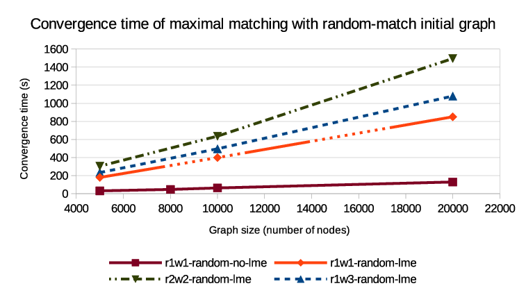
In this Appendix, for reader’s convenience, we provide graphical representation of the results in Section 5. Specifically, Figure 2 corresponds to some of the data in Table 2, and Figure 3 corresponds to some of the data in Table 4.



Appendix B Convergence Pattern of Maximal matching in the Experiments deployed on Amazon EC2 instances.
Figure 4 shows the convergence of maximal matching in the experiments deployed on Amazon EC2 instances. We note that the convergence pattern in Figure 4 is similar to the convergence pattern in Figure 1 except that the convergence in Amazon EC2 experiments converges slower. This is because the delay in Amazon AWS network is longer.