Fast tensorial JADE
Abstract
In this work, we propose a novel method for tensorial independent component analysis. Our approach is based on TJADE and -JADE, two recently proposed generalizations of the classical JADE algorithm. Our novel method achieves the consistency and the limiting distribution of TJADE under mild assumptions, and at the same time offers notable improvement in computational speed. Detailed mathematical proofs of the statistical properties of our method are given and, as a special case, a conjecture on the properties of -JADE is resolved. Simulations and timing comparisons demonstrate remarkable gain in speed. Moreover, the desired efficiency is obtained approximately for finite samples. The method is applied successfully to large-scale video data, for which neither TJADE nor -JADE is feasible. Finally, an experimental procedure is proposed to select the values of a set of tuning parameters.
1 Tensorial independent component analysis
In modern data analysis an increasingly common and a natural assumption is that the covariance matrices are Kronecker-structured: the random vector has a covariance matrix where , are positive-definite and is the Kronecker product. In order for an estimator of to be adequate, it should utilize this special structure, see e.g. Leng and Pan (2018); Roś et al. (2016); Srivastava et al. (2008); Werner et al. (2008); Wiesel (2012). In particular, if the Kronecker structure is ignored, the amount of parameters is inflated from to .
Basic properties of the Kronecker product ensure that any zero-mean random vector x, with the Kronecker covariance structure, admits a natural representation as a random matrix by means of the matrix location-scatter model,
where the original random vector is obtained from vectorization, , and the latent random matrix Z is standardized such that . In order to find interesting structures, the uncorrelatedness assumption for the elements of Z is occasionally not enough. In Virta et al. (2017) the uncorrelatedness assumption was replaced by the assumption of full statistical independence and the location-scatter model was extended to the matrix-valued independent component model,
| (1) |
where the invertible are unknown parameters and the latent tensor Z is assumed to have mutually independent, marginally standardized components. The estimation procedure of a latent vector with independent components, using only the information provided by observed linear combinations of the components, is referred to as independent component analysis (ICA). See Comon and Jutten (2010); Hyvärinen et al. (2004); Ilmonen and Paindaveine (2011); Miettinen et al. (2015); Nordhausen and Oja (2018); Samarov and Tsybakov (2004) for different approaches under classic multivariate settings. Since the location has no effect on the estimation of the so-called mixing matrices and , we can without loss of generality assume that Z is centered. Under the additional assumption that at most one entire row of Z has a multivariate normal distribution and at most one entire column of Z has a multivariate normal distribution, it can be shown that the latent Z is identifiable up to the order, joint scaling and signs of its rows and columns (Virta et al., 2017). This pair of assumptions is less restrictive than its counterpart in standard vector-valued ICA, which allows a maximum of one normal component in the latent vector (Comon and Jutten, 2010). On the contrary, the assumptions of the matrix model allow Z to contain up to normal components, if the non-normal elements are suitably located.
Vectorizing Eq. (1) yields a Kronecker-structured standard independent component model
where , . Again, here any reasonable ICA approach should take the special form of the mixing matrix into account. To our knowledge, no structured estimation methods have yet been developed for standard vector-valued ICA in this setting. However, the problem has been considered under the matrix representation of Eq. (1) in Virta et al. (2017); Virta et al. (2018), where two classical ICA procedures, fourth order blind identification (FOBI) (Cardoso, 1989) and joint diagonalization of eigen-matrices (JADE) (Cardoso and Souloumiac, 1993), are extended to TFOBI and TJADE in order to solve Eq. (1). Even though TJADE provides a definite improvement in efficiency with respect to TFOBI and the classical multivariate versions of the procedures, it is relatively expensive to compute. Consequently, the main goal of this paper is to address this issue. We provide a computationally more powerful, alternative TJADE-based estimator, which retains the desirable statistical properties of TJADE. In particular, the estimator retains the consistency and the limiting distribution of TJADE.
We wish to point out that the statistical models for matrix data we are about to discuss are markedly different from the ones usually encountered when discussing array-valued data in engineering contexts. The relevant engineering literature is populated mostly with different tensor decompositions, the most popular ones being the Tucker decomposition and the CP-decomposition, which extend the singular value decomposition to higher order structures in different ways, see Cichocki et al. (2015); Kolda and Bader (2009) for comprehensive reviews. A fundamental difference between the classical tensor decompositions and our current model is that the former rarely incorporate the concept of sample in the formulation. As such, tensor decompositions generally reduce also the dimension of the observation space which is very unusual for classical statistical methods. These fundamentally different objectives also prevent any simple, meaningful comparisons, and therefore we have refrained from including comparisons to classical tensor decompositions in this work.
The rest of the paper is structured as follows. In Section 2, we review the existing methodology on tensorial independent component analysis and, in particular, TJADE on which our proposed extension will be based. In Section 3, we formulate -TJADE in the case of matrix-valued observations and thoroughly establish its limiting behavior along with the necessary assumptions. The theoretical results are extended to a general tensor-valued model in Section 4 using the technique of matricization. Section 5 explores the finite-sample performance of the proposed method under both simulations and data examples on videos and hand-written digits. We also investigate the estimation of a set of tuning parameters of -TJADE in the context of the latter example. In Section 6 we provide a short summary and list ideas for future work. Technical proofs are presented in Appendix A.
2 Tensorial JADE
We begin by briefly describing the theory behind TFOBI and TJADE. Everything in the following is formulated on the population level for a random matrix . In practice, one would obtain a sample of matrices, , from the distribution of X and the expected values below should be replaced by sample means.
Assuming that the random matrix follows the model in Eq. (1), the first step is to simultaneously standardize both, the rows and the columns of the matrix, using the left and right covariance matrices of X,
We denote the unique symmetric inverse square root of the positive-definite matrix S by . The standardized variable satisfies for some and some orthogonal matrices, , see Virta et al. (2017). The unknown constant of proportionality is a result of the joint scaling of the model in Eq. (1) being left unfixed. After the standardization, solving the IC problem is reduced to the estimation of the orthogonal matrices , a task commonly addressed in ICA using higher-order cumulants. The TFOBI and TJADE procedures also utilize the higher-order cumulants. In TFOBI, a Fisher consistent (under mild assumptions, see Section 3) estimator, , for the inverse of the matrix is constructed such that
where the columns of are the eigenvectors of the matrix
Thus, provides a solution for the left-hand side of the IC model in Eq. (1) (Virta et al., 2017).
The TJADE procedure utilizes a set of matrices, , referred to as the set of cumulant matrices, such that
| (2) |
where is the Kronecker delta, , , are the standard basis vectors of and . The left covariance matrix of the standardized matrix satisfies and is included in Eq. (2) solely for the estimation of the constant of proportionality . The authors in Virta et al. (2018) proved that the joint diagonalizer of is under mild assumptions, see Section 3, equal to the orthogonal matrix up to the order and signs of its columns. The joint diagonalizer of the set is defined as any orthogonal matrix that minimizes
| (3) |
where is equal to with the diagonal elements set to zero.
The joint diagonalizer defines a coordinate system in which the linear transformations , , have minimal sum of squared off-diagonal elements. There exists several algorithms for optimizing Eq. (3), the most popular being the Jacobi-rotation technique, for details see Belouchrani et al. (1997); Illner et al. (2015). After the estimation of the joint diagonalizer , an estimated inverse for the matrix is obtained as the TJADE-fucntional, .
The results of this paper are derived only for the left-hand side of the matrix-valued model. The right-hand side of the matrix-valued model can be solved exactly as the left-hand side. One can simply take the transpose of X and proceed as with the left-hand side. Only the sizes of the cumulant and transformation matrices change from to . Moreover, matricization allows us to extend the estimators beyond the matrix-valued model to arbitrary-dimensional tensor-valued IC models, see Virta et al. (2017); Virta et al. (2018). Matricization allows us to hide a considerable amount of the unpleasant notation related to tensor algebra, see Section 4. In total, it is sufficient to present the results in matrix form and only for the left-hand side of the model in Eq. (1).
When the dimension is equal to one, the TJADE procedure for the left-hand side of the model is equivalent to the standard JADE for vector-valued data. Extensive comparisons between JADE and TJADE are conducted in Virta et al. (2016); Virta et al. (2017); Virta et al. (2018) with the conclusion that the latter is uniformly superior to the former under the Kronecker-structured IC model. Moreover, the tensorial version is computationally significantly faster. Consider a tensor of th order with all dimensions of size . Standard JADE requires a single joint diagonalization of matrices that are of size , whereas TJADE requires joint diagonalizations of matrices that are of size . In essence, adding dimensions to a tensor has a multiplicative effect on the number of operations the classic vectorial methods require and merely an additive effect on the tensorial methods. However, even with its considerable advantages over JADE, running the TJADE procedure is slow for large tensors.
To obtain a faster method, we approach the problem in the spirit of Miettinen et al. (2013) where a faster version of JADE, -JADE, is derived. The modification can be described very succinctly: instead of diagonalizing the entire set of cumulant matrices , we diagonalize only a specific subset of them, chosen such that the desirable statistical properties of TJADE are still carried over to the extension. Since the subset of cumulant matrices can be chosen separately in each direction of the tensor, the -JADE approach provides even more significant improvements in tensorial settings compared to its original use in improving JADE. Note that, similar ideas as in Miettinen et al. (2013) were used already in Cardoso (1999) to formulate shifted blocks for blind separation (SHIBBS), where only those cumulant matrices of regular JADE with matching indices are diagonalized.
3 Tensorial -JADE
In this section we propose a novel extension of the TJADE procedure. We formulate the extension, -TJADE, such that it retains the following three key properties of TJADE. The first of these properties is the ability to solve the tensor independent component model, manifesting either as Fisher consistency or consistency, depending on whether we are at the population or sample level, respectively. The second property is orthogonal equivariance under arbitrary data. ICA-estimators are customarily expected to have some form of equivariance, which makes the generalization of limiting properties more straightforward (Miettinen et al., 2015; Virta et al., 2017). The third desired property is the limiting distribution of TJADE, the one with the lowest limiting variance of the known tensorial ICA methods. Next, we establish these properties one-by-one. As mentioned in the previous section, all results derived for the left-hand side of the model also hold for the right-hand side, prompting us to consider only the former in the following. In the same spirit, even though the proposed -TJADE method has in the case of matrix data two tuning parameters, for the rows and for the columns, the method still acts only on a single mode at a time, and as such we omit the subscripts and speak in the following only of the tuning parameter . Moreover, the same idea is reflected in the name of the method which should (for matrix data) technically be -TJADE. In order to keep the presentation more readable, we prefer to call the method simply -TJADE.
We define matrix independent component functionals, the extension of independent component functionals (Miettinen et al., 2015) to matricial ICA.
Definition 1.
A matrix-valued functional is a matrix independent component (IC) functional if
- (i)
for all that follow the matrix IC model of Eq. (1),
- (ii)
for all and all orthogonal , ,
where two matrices satisfy if for some , some diagonal matrix with diagonal elements equal to and some permutation matrix .
The first condition in Definition 1 requires that a matrix IC functional must be able to solve the left-hand side of the model in Eq. (1) (Fisher consistency). The second condition essentially states that the functional cancels out any orthogonal transformations on the observed matrices (orthogonal equivariance). As a particularly useful consequence of the latter, the limiting distribution of a matrix IC functional under trivial mixing, , , instantly generalizes to any orthogonal mixing as well.
Let be the vector of the row means of the element-wise kurtoses, , of the elements of Z.
Assumption 1.
At most one element of equals zero.
Assumption 2 ().
The multiplicities of the elements of are at most .
The TFOBI functional is a matrix IC functional in the sense of Definition 1 if Assumption 2 is satisfied and the TJADE functional is a matrix IC functional if Assumption 1 is satisfied. Naturally, the column mean analogues of the assumptions are required to separate the right-hand side of the model in Eq. (1).
The same comparison as was done between the normality assumptions in Section 1 holds analogously between Assumption 1, Assumption 2 and their vectorial counterparts allowing maximally one zero-kurtosis component or only distinct kurtoses, respectively. The main implication is that in matrix ICA numerous latent components may have identical kurtoses as long as their row means (and column means when separating the right-hand side of the model) satisfy the necessary requirements. The assumptions also satisfy the following set of relations,
where means “implies”. Moreover, we have also .
In order to speed up TJADE such that the properties in Definition 1 are retained, we proceed as in Miettinen et al. (2013), and instead of diagonalizing the set , we diagonalize only those members of it which satisfy , for some pre-defined value of the tuning parameter . This discarding can be motivated in two ways. Firstly, all except the repeated index matrices, , vanish asymptotically. Every matrix , , implying that with increasing sample size all the separation information is eventually contained in the repeated index matrices. Secondly, by assuming that the values in are in decreasing order (this is guaranteed by using TFOBI as a preprocessing step, see the next paragraph) the th row of Z is the most difficult to separate from its immediate neighboring rows and the separation information between them is contained precisely in the matrices and where is close to .
Analogously to -JADE, we use the TFOBI-algorithm to obtain an initial value for the functional. This ensures that even after the previous modification, the functional remains orthogonally equivariant. The following definition and theorem formalize our resulting novel method, called -TJADE.
Definition 2.
Fix . The -TJADE functional is
where is the TFOBI functional, is the TFOBI-solution for X and the orthogonal matrix is the joint diagonalizer of the set of matrices
Theorem 1.
Theorem 1 provides the Fisher consistency and the orthogonal equivariance for the -TJADE functional. The assumptions that Theorem 1 requires are interesting since they provide an interpretation for the tuning parameter — the parameter is the maximal number of allowed kurtosis mean multiplicities. The values and correspond to the extreme cases where all the kurtosis means have to be distinct (as in TFOBI) and where no assumptions are made on the multiplicities of the non-zero kurtosis means (as in TJADE). Thus, -TJADE can be seen as a middle ground between TFOBI and TJADE. As the assumptions, also the methods can be ordered according to the strictness of the assumptions they require,
where “” is read as “makes at least as many assumptions as” and “” as “makes the same assumptions as”.
We next give some intuition behind the proof of Theorem 1 (given in Appendix A). The proof relies on a specific interplay between the preliminary TFOBI-step and the set of cumulant matrices . Being an eigendecomposition-based method, TFOBI is able to estimate the matrix only up to row blocks determined by the elements of , such that the rows of the estimate corresponding to equal kurtosis values remain mixed by orthogonal matrices (c.f. eigenvectors corresponding to multiple eigenvalues are not uniquely defined but their span is). However, the proof also shows that the joint diagonalization of all cumulant matrices with , for some given , can separate mixed row blocks of size at most (intuitively, increasing means using more cumulant matrices which increases the amount of available information). Thus, by sequencing the two steps together and having ensures that any blocks left still mixed after the TFOBI-step will be unmixed in the joint diagonalization step.
Assumptions 1 and 2 not only provide Theorem 1, but are also sufficient to guarantee the two remaining desired properties of -TJADE, consistency and the same limiting distribution as that of TJADE. These asymptotic properties are formalized in the following two theorems. Remarkably as a special case, when , the latter also proves a previously unsolved conjecture posed about the limiting behavior of vectorial -JADE in Miettinen et al. (2015).
Theorem 2.
Let Assumptions 1 and 2 hold for some fixed and let be an i.i.d. sequence from the matrix IC model in Eq. (1) with identity mixing matrices, . Assume that the population quantity X has finite eight moments. Then, for all , there exists a consistent sequence of -TJADE-estimators (indexed by ). That is,
Theorem 3.
Under the assumptions of Theorem 2, we have for all that,
where is the TJADE-estimator. The notation refers to a sequence of random matrices that converges in probability to the zero matrix.
The proofs of Theorem 2 and 3 are based on the fact that the kurtosis matrices of the latent Z with non-matching indices vanish asymptotically, , . The key point of the proof is then to show that this property transfers to the corresponding kurtosis matrices , of the TFOBI-standardized observation, to such extent that the asymptotical contribution of the sample estimates of these matrices to the final -TJADE estimate is negligible. Thus, regardless of the choice of , the asymptotical behavior of the method is determined by the repeated index matrices . Finally, the proof reveals that the rotation specified by the joint diagonalization dominates over the preliminary TFOBI-rotation and the effect of the latter also turns out to be asymptotically negligible.
Note that, does not generally hold as the latter estimator utilizes the preliminary TFOBI-step while the former does not. The limiting distribution of is in Virta et al. (2018) shown to be multivariate normal and closed form expressions for its limiting variances are also given therein. By the orthogonal equivariance of matrix independent component functionals (property (ii) of Definition 1) the limiting results of Theorem 3 generalize to any orthogonal mixing matrices. Note that the original -JADE in Miettinen et al. (2013) is affine equivariant (equivariant under all coordinate system changes, not just orthogonal). The problem of achieving affine equivariance in the context of tensorial ICA is discussed in Virta et al. (2018). There it was conjectured that tensorial ICA cannot be affine equivariant.
The two limiting theorems above show that, under suitable assumptions, -TJADE indeed has all the desirable properties listed at the beginning of this section. This can be summarized by saying that -TJADE makes a trade-off between assumptions and computational load: with the price of added assumptions, we obtain a method with the same limiting efficiency as TJADE, but with significantly lighter computational burden. As the claim about efficiency holds only asymptotically, we conduct a simulation study (in Section 5) to compare the finite-sample efficiency of the estimators.
Note that the maximal kurtosis multiplicity is unknown in practice, which makes the choosing of such that a non-trivial task. However, the simulations of Section 5 reveal that not a lot of separation efficiency is necessarily lost when using a slightly too small value of , making the problem less dire. To further alleviate the issue, in the final part of Section 5, we propose a procedure for estimating and apply it to hand-written digit data.
4 A note on tensorial ICA
In this section, we formulate the general tensorial IC model and discuss how it can be reduced to the matricial IC model. We begin with a short review of the basic concepts of multilinear algebra.
An th order tensor is an -dimensional array containing a total of elements and has a total of modes or ways, that is, directions from which we can view it. For example, a matrix () can be viewed either through its columns or through its rows. Two complementary ways of dividing a tensor into a disjoint collection of smaller tensors are called the -mode vectors and the -mode faces. In the former, we choose an index and have the values of the indices fixed and let the th index vary over its range. Each fixed combination of the indices then yields a single -dimensional vector and the collection of all such vectors is called the set of -mode vectors of . On the other hand, if we fix the value of the th index and let the others vary over their ranges, we get a total of tensors of order and size , called the -mode faces of . Illustrations of both, -mode vectors and -mode faces, , in the case of a 3-dimensional tensor, are shown in Figures 1 and 2.


Two algebraic operations can now be defined in terms of the -mode vectors. Let and for some fixed . The -mode multiplication of from the th mode by is defined element-wise as,
The -mode multiplication is easily understood: is obtained by multiplying each -mode vector of from the left by and collecting the resulting vectors back into an -dimensional tensor in the same order. The -mode multiplications from distinct modes are commutative and we use the shorthand . In the case of matrices, , the simultaneous multiplication from both modes simply gives .
To show the connection between the matricial and tensorial IC methods, we still need the concept of -mode matricization. For a fixed mode , the -mode matricization of is obtained by taking the -mode vectors of and collecting them horizontally into a wide matrix. The arrangement order of the -mode vectors has no effect on our further developments, and we choose to use the cyclical ordering as in De Lathauwer et al. (2000). In this case the relationship,
| (4) |
holds. For more comprehensive introduction to multilinear algebra, see Cichocki et al. (2009); De Lathauwer et al. (2000).
We are now sufficiently equipped to examine the connection between the matricial ICA and the tensorial ICA. The zero-mean th order random tensor is said to follow the tensorial independent component model if
| (5) |
where the random tensor has mutually independent, marginally standardized components and , , are invertible (Virta et al., 2017). We further assume that for each mode at most one -mode face of consists solely of normally distributed components. The objective of tensorial independent component analysis is to estimate given a random sample of observed tensors from the distribution of .
We fix the mode and consider the -mode matricization of the model in Eq. (5). It now follows from Eq. (4) that
| (6) |
As Kronecker products of invertible matrices are themselves invertible, a comparison to Eq. (1) now reveals that Eq. (6) is in the form of a matrix IC model with replacing and taking the role of . In addition, satisfies all the assumptions of the matrix IC model. To be precise, it is possible that multiple columns of have multivariate normal distributions as a consequence of the matricization. However, as the -mode matricization leaves the structure of the th mode intact, the normality assumption on guarantees that at most one row of has a multivariate normal distribution, which is then sufficient for the identifiability of , the current parameter of interest. Thus, using Eq. (6), we can estimate exactly as in the matricial case. In the tensorial case, the kurtosis means in the vector in Assumption 1 and in Assumption 2 are computed over the rows of , or equivalently, over the -mode faces of . All our theoretical results, such as orthogonal equivariance (a Kronecker product of orthogonal matrices is itself orthogonal) and the asymptotic variances, hold fully under the tensorial IC model, as long as the relevant kurtosis assumptions are satisfied. Finally, we remind that for an th order input tensor , the -TJADE has a total of tuning parameters, , with the underlying idea that should be chosen to be equal to or larger than the maximal kurtosis multiplicity in the corresponding mode, see Theorem 3.
5 Simulations and examples
In this section, we illustrate the finite sample properties of the tensor-valued procedures TFOBI, TJADE and the novel -TJADE, which are implemented in the R-package tensorBSS (Virta et al., 2016). For comparison, we also consider the classical vector-valued versions of these estimators, denoted by VFOBI, VJADE and -VJADE, as implemented in the JADE package (Miettinen et al., 2017). In the classical procedures, the tensor-valued observations are first vectorized and the algorithms are then applied to the resulting data matrices.
Next, we consider a collection of observed i.i.d. tensors , generated from the tensorial independent component model, such that , for every . Let be the theoretical mixing matrices and let be the corresponding unmixing estimates produced by one of the tensor-valued procedures. We denote the Kronecker products of the matrices as and . The vector-valued procedures produce a single unmixing estimate, denoted also by . Note that the estimates produced by the vectorial and the tensorial methods are comparable, since in both cases the matrix estimates the inverse of the compound matrix .
The so-called gain matrix is defined as . The unmixing is considered successful if the gain matrix is close to the identity matrix, up to the order and signs of its rows. We quantify this closeness using the performance measure called minimum distance (MD) index (Ilmonen et al., 2010). The MD index is formulated as follows,
| (7) |
where and is the set of all matrices with exactly one non-zero element in each row and column. The range of the MD index is , where the value corresponds to the case of the gain matrix being exactly a permuted and scaled identity matrix, i.e. the estimate is perfectly accurate. Additionally, the limiting distribution of the MD index can be obtained from the limiting distribution of the corresponding IC functional , see (Ilmonen et al., 2010, Theorem 1) and (Virta et al., 2017, Theorem 6).
In simulation studies, where multiple iterations are performed under identical conditions, the asymptotic value for the mean of the transformed MD index can be obtained using the limiting variances of the applied IC functionals, see Virta et al. (2017) for further details. The convergence towards the theoretical limiting values given by Theorem 3 can then be demonstrated by visualizing the theoretical limits alongside , where is the number of iterations for the sample size and is the estimated gain matrix for the corresponding th iteration.
Before presenting the simulations, we discuss shortly the importance of the tuning parameter , which in -TJADE can be chosen separately for each mode. In the following, -TJADE is used to refer to -TJADE with the value for the tuning parameter in the th mode, . Based on Theorem 3, the computationally cheapest but still asymptotically optimal choice is the largest multiplicity of the kurtosis means in the current mode. This means that we have generally three choices for each mode: we may use the full TJADE if the mode is short; we can use -TJADE for some small if the mode is long; or we can choose not to separate the mode at all if it is not expected to contain any relevant information, as might be the case, e.g., for the color dimension of a sample of images.
5.1 Finite-sample efficiency, setting 1
We begin by demonstrating that the finite sample performance of -TJADE is in line with the asymptotic results given in Theorem 3. In the first setting, we consider simulated collections of i.i.d. matrices of size , . The components of every are simulated independently from the following distributions,
where C, E, U and N denote independent replicates from the , standard exponential, uniform and normal distribution, respectively, all scaled to have zero mean and unit variance.
In this simulation setting, none of the theoretical row or column kurtosis means are zero. However, the theoretical mean kurtoses are the same for the first two rows and the first two columns. Thus, the preferable -TJADE procedure here is 22-TJADE, . Note that in this setting the requirements of TFOBI are not fulfilled.
When the observations are vectorized, the length nine vectors contain a single normally distributed component, two -distributed elements, three elements from the exponential distribution and three elements from the uniform distribution. The vector now contains one element (the normally distributed component) with theoretical kurtosis 0, making vectorial ICA viable. The most natural -VJADE procedure here is 3-VJADE. The assumptions of VFOBI are violated.
The simulation was performed using 13 different sample sizes, , with repetitions per sample size. To evaluate the equivariance properties and the effect of non-orthogonal mixing, we mixed the observations at each repetition using (i) identity mixing: , (ii) orthogonal mixing: and , where and are random orthogonal matrices uniformly sampled at each repetition with respect to the Haar measure and (iii) normal mixing, where and were filled at each repetition with random elements from .
To evaluate the effect of the mixing matrix and the limiting distributions, we present, in Figure 3, the transformed MD values for 3-VJADE, VJADE, 22-TJADE and TJADE and the corresponding theoretical limit values for the cases available. As our theory extends only the orthogonal mixing, the theoretical limit value of TJADE is missing from the third panel. The sample sizes , , are omitted from Figure 3, since the sample size is large enough for the convergence of both the vectorial and the tensorial methods.
Figure 3 clearly shows that for the vectorial methods, we have affine invariance and thus all of the three curves are identical. For the tensorial methods, we have only orthogonal invariance and hereby the curve corresponding to the normal mixing differs from the other two. Moreover, despite the limiting value of TJADE being unknown for normal mixing, based on the finite-sample curves, it seems that normal mixing does not change the relative separation accuracy of the tensorial methods over orthogonal mixing. Only the overall separation difficulty level is affected (the curves are higher in the plots). Furthermore, the benefit of applying the tensorial methods over the vectorized methods is impressive. Finally, Figure 3 also illustrates that all the methods converge to the theoretic values and that the -TJADE versions have the same limiting values as TJADE.
We next, under the same setting as above, present the results for seven additional procedures that violate some of the required assumptions: VFOBI, TFOBI, 1-VJADE, 2-VJADE, 11-TJADE, 12-TJADE and 21-TJADE. Note that TFOBI is the initial step in the -TJADE procedure and hereby the comparison between -TJADE and TFOBI illustrates the added benefit of the additional rotation after the TFOBI-solution. Likewise, the same holds between VFOBI and -VJADE. The resulting mean values of the transformed MD indices are presented in Figure 4, where methods that have almost identical performance are presented using the same colors.
In Figure 4, TFOBI and VFOBI diverge at an exponential rate. Furthermore, the -TJADE procedures that have either or less than the number of distinct kurtosis values, are not converging to anything reasonable, even at sample sizes greater than . However, in this simulation setting, the -VJADE procedure seems to allow slight deviations from the required assumptions. It seems that 2-VJADE converges to an asymptotic value that is at least close to that of VJADE, see Section 6 for further discussion.
To summarize this part of the simulation study: -TJADE works as expected, when the theoretical conditions are met, and the convergence to the asymptotic value is relatively fast. Furthermore, even though -TJADE is not affine invariant, its performance is better under all mixing scenarios, when compared to the affine invariant vectorial counterparts.
5.2 Finite-sample efficiency, setting 2
In our second simulation, we illustrate unmixing under a tensorial setting. We consider simulated collections of i.i.d. tensors of size , . Let denote the th 3-mode face of . The components of every are then simulated independently from the following distributions,
where the different distributions are denoted as in Section 5.1.
All of the mean kurtoses over the different tensor faces are nonzero and none of the theoretical mean kurtoses are the same for the 1-mode faces. Moreover, two of them are the same for the 2-mode faces and three of them are the same for the 3-mode faces. Hereby, the preferable -TJADE here is -TJADE, . The vectorized versions of the observations contain several normal components and thus the assumptions for the vectorial methods are not satisfied here.
The simulation was performed using 11 different sample sizes, , and the simulation was repeated 2000 times for each sample size. We considered the same three mixing scenarios as in Section 5.1 and generated the mixing matrices in the same way, with the distinction that here we have three mixing matrices instead of two. We performed the unmixing using VFOBI, TFOBI, 1-VJADE, 2-VJADE, VJADE, TJADE and 11 different versions of -TJADE. The resulting mean values of the transformed MD index, , where and , are presented in Figure 5. The orthogonal mixing is omitted from Figure 5, since the tensorial methods are orthogonally invariant and the vectorial methods are affine invariant. The performance curves under the orthogonal mixing would be identical to those under the identity mixing, similarly as in Section 5.1.
The -TJADE performs as expected for the values of that satisfy the assumptions and the convergence towards the theoretical limit is considerably fast. The vectorial methods fail completely in this example. Interestingly, -TJADE has relatively nice performance when the elementwise deviation between and (1,2,3) is not too large. See Section 6 for further discussion.
5.3 Finite-sample efficiency, setting 3
In the third simulation setting, we have a collection of i.i.d. matrices , with components simulated independently from the following distributions,
where denotes the gamma distribution, with shape parameter and rate parameter 1, scaled to have zero mean and unit variance. The theoretical row kurtosis means are approximately,
and the theoretical column kurtosis means are approximately,
Hereby, in this simulation setting, the row kurtosis means are very close to each other. They start to differ at the fourth decimal. Also the column kurtosis means are quite close to each other.
The simulation study was conducted exactly as in Section 5.1, with the distinction that the largest sample size of Section 5.1 was omitted here. Furthermore, we had more versions of -TJADE in this study. The results are displayed in Figure 6.
Theoretically, the preferable -TJADE would be 11-TJADE, . However, with the current sample sizes, 11-TJADE, 12-TJADE and 13-TJADE do not seem to converge, see Figure 6. Similarly, 21-TJADE and 31-TJADE exhibit erratic behavior with small sample sizes. Yet, with sample sizes over one million, the corresponding procedures are very close to the theoretical limiting value, given as the solid black line in Figure 6. It seems that with sample sizes of magnitude , differences in column kurtosis means that are of magnitude , are not a problem for the procedures. Conversely, the current sample sizes are not large enough to compensate the small differences in the row kurtosis means.
The curves corresponding 22-TJADE, 23-TJADE, 32-TJADE and TJADE behave nicely in Figure 6, even with relatively small sample sizes. Especially, the good behavior of 22-TJADE is a little surprising. The corresponding procedure assumes that at most two of the column kurtosis means and at most two of the row kurtosis means are equal. We wish to emphasize that the assumptions required for the -TJADE procedures are only sufficient conditions and it can be that in some special cases, e.g., under some special distributional structures, some of the procedures behave well, even though the sufficient assumptions are not satisfied.
In Figure 6, the curves that correspond to VFOBI and TFOBI are again only visible in the top left corner. This is unsurprising since the required assumptions are not satisfied for VFOBI, and TFOBI cannot handle the close kurtosis means, even though they are distinct on the population level. With the current sample sizes, 1-VJADE does not seem to converge to the theoretical limiting value, given as the dashed black line. The vectorial 2-VJADE, 3-VJADE and VJADE seem to function quite well in this setup. This could be explained by the fact that the vectorial methods have assumptions directly related to the theoretical kurtoses of the components, whereas the tensorial methods have assumptions related to means of the kurtoses. It is easier to detect small kurtosis differences, when compared to detecting differences in their means.
5.4 Timing comparison
The results from Sections 5.1 and 5.2 illustrate that the performances of TJADE and suitably chosen versions of -TJADE are very similar. Next, we quantify the significant improvement in computational speed that -TJADE provides when compared to TJADE. In the timing comparison, we consider a simulated collection of i.i.d. matrices of size , , such that components of every are simulated independently from the following distributions,
where denotes the -squared distribution with degrees of freedom, and the width of the matrix is the varying parameter in this simulation setting. We used parameter values and the sample size . We considered the same procedures as in Section 5.1: VFOBI, TFOBI, 1-VJADE, 2-VJADE, 3-VJADE, VJADE, 11-TJADE, 12-TJADE, 21-TJADE, 22-TJADE, TJADE and recorded the mean running times over a total of 5 iterations. The time it took R to vectorize the tensors was also considered as a part of the vectorized procedures. However, the time the vectorizing took, was negligible. We used two alternative stopping criteria for the methods that involve joint diagonalization, that is, for all the methods except for TFOBI and VFOBI. A single iteration was stopped, if either the converge tolerance of the Jacobi rotation based joint diagonalization was less than or if the required tolerance was not satisfied after 100 iterations.
The average running times in minutes as a function of the dimension are presented in Figure 7 and methods that have almost identical computing times, are presented using the same colors. Figure 7 clearly illustrates the superior computation speed of -TJADE, when compared to either TJADE or any of the vectorized counterparts. The timing comparison was conducted on Ubuntu 16.04.4 LTS with Intel® Xeon® CPU E3-1230 v5 with 3.40GHz and 64GB.
5.5 Video example
We applied -TJADE to the WaterSurface surveillance video (Li et al., 2004) that is viewable at http://pages.cs.wisc.edu/~jiaxu/projects/gosus/supplement/ and available to download as an .Rdata file at https://wis.kuleuven.be/stat/robust/Programs/DO/do-video-data-rdata. The video has already been used as an example for blind source separation (Virta and Nordhausen, 2017a; Virta and Nordhausen, 2017b). Each frame of the video is of size with the height , width and a three-variate color channel (RGB). The total video consists of such frames, making our data a sample of size of random third order tensors in . The data constituting a single continuous surveillance video, the observations are naturally not independent and the assumptions of tensorial independent component analysis are not fully satisfied. However, ICA is known to be robust against deviations from the independence assumption and applying it to sets of dependent data with success is common practice. We thus expect -TJADE to successfully extract components of interest from our current data.

The video shows a beach scene with little to no motion until frame 480, when a man enters the scene from the left, staying in the picture for the remainder of the video. Figure 8 shows frames 50 and 550 of the video, illustrating moments before and after the man enters the scene. Our objective with the surveillance video is to find low-dimensional components that allow us to pinpoint the most obvious change point in the video, namely, the man’s entrance. As change points are most likely captured in the data as outliers of some form, it is natural to seek the component of interest among those with high kurtosis values.
We proceed as follows: we run -TJADE on the data with different choices of the tuning parameters, find the component with the highest absolute kurtosis, and plot its time course to visually assess whether it captures the change point. The component found with -TJADE is shown in Figure 9, where means that we do not unmix the supposedly uninformative color dimension at all. The time series is instantly seen to capture the desired time point as the spike coincides with the first frames the man spends in the scene. The running time of the method was 39 minutes on a Windows server with Intel® Xeon® CPU R5 2440 with 2.40GHz and 64GB. Applying -TJADE gave almost identical results with the increased running time of one hour and 54 minutes. However, the original TJADE proved to be very slow. The running time of the algorithm was over five days. Concluding, the example shows that -TJADE can be used to reliably extract information from data where TJADE can not be applied due to its extremely high computational cost. In several real world applications, e.g. in crime scene investigation, waiting for days is not an option.
5.6 Estimation of the maximal kurtosis multiplicity
In the previous video example, applying -TJADE already gave satisfactory results in the sense that it allowed us to find a latent component identifying the point of interest in time. However, in some cases, using the preferable value for the tuning parameter might be justified. This will guarantee the successful estimation of all components, while simultaneously keeping computation times and the amount of noise in the estimation minimal. The results of Theorem 3 could possibly be used to formulate an asymptotic hypothesis test for the null hypothesis that for some given in a given mode. Namely, if the null hypothesis holds, then the limiting distributions of the unmixing estimates are identical, allowing us to pin-point the true value of . In the following, we will pursue this idea from an empirical perspective and develop a heuristic procedure for the estimation of .
Consider a fixed mode of size of a sample of data from the tensorial IC model in Eq. (5) and let be the unmixing matrices estimated from the corresponding data, respectively, to -TJADE with the value of . Letting be the true maximal kurtosis multiplicity in the data, we thus expect to separate the data well but to leave some parts still unmixed (within the multiplicities). Analogously, we expect , where is the MD index in Eq. (7), to be large as the two matrices should have structures differing beyond row permutations, scaling and sign changes (in the extreme case where we have ). On the other hand, we expect all the following sequential MD indices, , , to be small as all values of are sufficient for the separation, and yield asymptotically equal solutions.
The true value of can now be located by plotting versus and finding the value, starting from which the curve stays roughly constant. However, since using a single sequential MD index per value of might leave us with a curve that is not smooth enough to accurately distinguish the true , we compute, for each , the average of the forward sequential MD indices:
The plot of versus can be used to find the true value of similarly as with the plot of versus , and has the interpretation of quantifying the efficiency loss one encounters when using a particular value of , relative to the choice . Note also that the choice of can be done individually for each mode in the sense that the value of in -TJADE is invariant to the choice of , and similarly for higher order data.
To illustrate the proposed tool, we consider the hand-written digit data set from the R-package ElemStatLearn (Halvorsen, 2015). The data set consists of 7291 images of hand-written numerals 0–9 digitized to matrices, with each element in , describing the grayscale intensity of the corresponding pixel. The underlying objective of the data set is to build a classifier that can correctly identify the digits that each of the matrices represent. For simplicity, we work on a subset of 400 randomly chosen images of the digits 1 and 7. These two digits were chosen as their visual similarity makes the classification task more difficult. In this kind of context, ICA is commonly used as a preprocessing step to reduce the data into a low-dimensional subspace, which hopefully contains all the classification information, simplifying the task for the subsequent classifier. In this spirit, we apply the proposed estimation strategy for to the sample and obtain the two plots shown in Figure 10. The plots should be interpreted similarly as the scree plot in PCA, where the aim is to find an “elbow” where the slope changes quickly. The two curves seem to imply that the correct parameter for -TJADE is roughly . In Figure 11 we plot the components with the indices and of the -TJADE solution. These components were chosen as -TJADE orders the rows/columns in descending order according to their mean kurtoses, and low kurtosis is often a sign of bimodality, making it natural to search for components with classifying ability in the lower-right corner of Z. Indeed, the chosen components reveal a clear separation of the digits. All ones are concentrated roughly in one spherical cluster, with a single outlying seven inside. The bulk of the sevens lies around the cluster of ones in a curved manner and the location of an individual seven is based on the angle of its stem. The analysis could further be continued from here by fitting a classifier, for example, a support vector machine, to the obtained components.
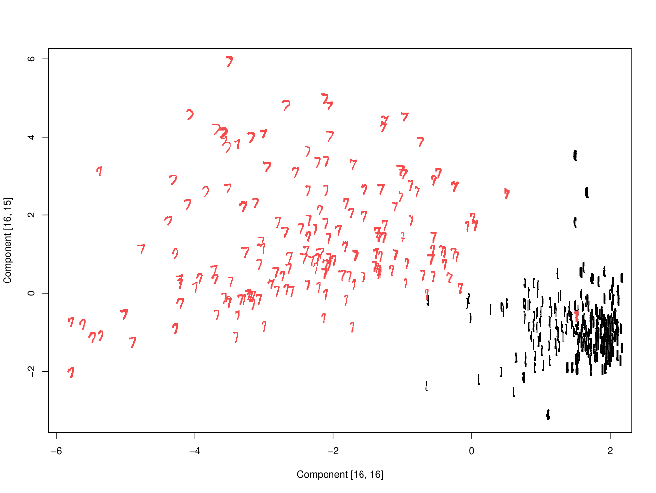
We conclude with two remarks. First, experimenting reveals (not shown here) that also, e.g., -TJADE finds similar separation of the two groups as is shown in Figure 11. There are two explanations for this: On one hand, locating the elbows in the scree plots in Figure 10 is visually difficult for a sample size this low, and thus it could be that is the actual optimal choice. On the other hand, whatever the true value of is, using larger than that is sure to guarantee that all independent components are estimated (asymptotically) correctly. However, it could be that the group separation structure is such a strong feature of the data that it can be found also with a sub-optimal choice of , and that using the optimal value of just guarantees that also the other (possibly less interesting) components are recovered successfully.
Second, the suggested procedure is somewhat excessive, as it requires the computation of the -TJADE solution for a wide range of values of . In addition, after having computed the solutions, one option would be to simply continue the analysis using the solution with the largest value of and ignore the estimation altogether. However, when dealing with very low sample sizes, it could happen that using a too large , although asymptotically sufficient for the estimation of all components, induces noise in the estimation. Still, the suggested procedure could prove useful in studies where a pilot/training data set is used to determine the optimal value of , which is then used for later data sets, saving computation time for all other data sets at the expense of the first. Finally, one option to save computation time would be to compute the values of sequentially, increasing one-by-one, and stopping when a significant drop in the plot is visible.
6 Discussion
We proposed a sped-up version of TJADE, the method with the lowest limiting variance among the currently studied methods of tensorial independent component analysis. Under easily interpretable additional assumptions, the extension, -TJADE, achieves the same limiting variance to TJADE, while simultaneously exhibiting significantly lower computational cost. A large part of this efficiency is preserved also for samples of finite size.
An interesting future research question is to derive the theoretic behavior of -TJADE when Assumption 2 is violated. Based on our simulations, even when the value of is chosen to be too small or too large, -TJADE and -JADE can still work. This can be seen as a safety net for the users of -TJADE. The simulations suggest that the performance deteriorates the further down one goes from the optimal .
Acknowledgements
The work of Joni Virta was supported by the Academy of Finland (grant 321883). The work of Niko Lietzén was supported by the Emil Aaltonen Foundation (grant 170156 N). The work of Klaus Nordhausen was supported by Austrian Science Fund (FWF) Grant number P31881‐N32 and CRoNoS COST Action IC1408. All authors acknowledge the computational resources provided by the Aalto Science-IT project.
The authors wish to express their gratitude to the two anonymous referees, whose insightful comments greatly helped improving the quality of the manuscript.
Appendix A Proofs
We denote the sequence of i.i.d. observations as , such that e.g. denotes the left sample covariance matrix estimated from the sample .
Before the proofs of the main results, we establish three auxiliary lemmas.
Lemma 1.
The minimization problem is equivalent to the maximization problem , where ,
Proof of Lemma 1.
Note that for all ,
Thus, is equivalent to
∎
Lemma 2.
For all and any orthogonal matrix , the sample and the population cumulant matrices satisfy,
| (8) | ||||
where denotes the sample .
Proof of Lemma 2.
Both results follow by the same arguments and we prove only the former. Since is a scalar and , the left-hand side of Eq. (8) can be written as
| (9) |
where the first term can be written as
| (10) |
where the -scaled expected value is the first term in the definition of the matrix and has the representation
| (11) |
Plugging Eq. (11) into Eq. (10) we obtain
| (12) |
Furthermore, plugging Eq. (12) into Eq. (9) gives us,
| (13) | ||||
Element-wise examination reveals that,
This concludes the proof. ∎
Lemma 3.
Let be a sequence of estimators (indexed by ) such that , where denotes convergence in distribution, is some matrix-valued distribution and
where and the values , , are distinct and in a strictly decreasing order (). Let be the sequence of eigenvector matrices, where the columns are the eigenvectors of the matrices . Partition into blocks as
in a similar way to . Then
Proof of Lemma 3.
The sequence of eigenvectors satisfies the eigenequation
| (14) |
where is a sequence of diagonal matrices containing the estimated eigenvalues. Then,
| (15) |
where the second equality holds since as a result of the compactness of the space of orthogonal matrices and since, by Prohorov’s theorem, our assumption implies that .
It follows from (Eaton and Tyler, 1991, Theorem 3.2) that , and consequently we obtain
| (16) |
By combining Eqs. (15) and (16) with Eq. (14), we arrive at
If this is written block-wise, we obtain
The result now follows by considering only the off-diagonal blocks, , and dividing by the non-zero . ∎
Remark 1.
In the sequel, the assumption of Lemma 3 that is fulfilled by applying central limit theorem.
Proof of Theorem 1.
By (Virta et al., 2017, Theorem 1) the standardized matrix satisfies for some and for some orthogonal matrices, . By (Virta et al., 2017, Eq. (5)) the TFOBI-matrix functional has the form,
where, are the row means of the kurtosis values of such that . Let be the number of the distinct eigenvalues of . Denote these distinct values by and denote the corresponding multiplicities of these values by , respectively. Note that each can be given as for some . As , where is the largest multiplicity among the row mean kurtoses , we have that , for all .
The set of eigenvectors of is identifiable up to orthogonal transformations within each eigenspace. That is, ignoring the order and signs, the eigenvector matrix of has the form
| (17) |
where each , , is orthogonal. The FOBI-rotated data is then
The proof of Theorem 1 is divided into two parts. First, we prove that the condition (i) in Definition 1 holds and after that we prove that the condition (ii) holds.
Condition (i):
The condition (i) claims that -TJADE can, under Assumptions 1 and 2, estimate the block diagonal orthogonal matrix up to the signs and the order of its columns. For convenience, we drop all subscripts referring to the side (left or right) of the model, e.g. in the following is and is H.
Adapting the proof of (Virta et al., 2018, Theorem 1), we have that
| (18) |
where is diagonal matrix for every . Since , the matrix H is a solution to the k-TJADE minimization problem
Next, we show that H is a unique minimizer, up to the signs and the order of its columns. Let such that and let be the subset of the index set for which the corresponding columns of H belong to the th eigenvalue block. By (Bonhomme and Robin, 2009, Lemma 2), the minimizer is unique up to the signs and order of its columns if, for each pair of distinct columns of H, there exists a pair such that the eigenvalues of corresponding to and are distinct. By the decomposition in Eq. (18), this is equivalent to requiring that
| (19) |
We next show that Eq. (19) holds for all by considering separately the two cases where and either belong to two different sets or where and belong to the same set of the partition .
First, assume that and belong to different sets of the partition. We proceed with proof by contraposition and assume that Eq. (19) does not hold. That is, for all , , the eigenvalue pairs are always equal. In particular, for all . By summing over the equations, we have, from the orthogonality of H, that , where . This implies that , which is a contradiction since we assumed that and belong to different sets of the partition and thus have different eigenvalues. Consequently, Eq. (19) holds for any pair of columns belonging to distinct sets of the index partition.
Assume then that and belong to the same set of the partition. We again proceed with proof by contraposition and assume that Eq. (19) does not hold. Now, and we have that for all , . In particular, this holds for all in the subset
| (20) |
By Assumption 2 and consequently the distance is always less than in the set . Hereby, the intersection in Eq. (20) is equal to . We now multiply each equality , with indices in the set , by . By summing twice over , we obtain
| (21) |
The constant . The constant , as the contrary would imply that two of the kurtosis values were equal to zero, , which would then contradict Assumption 1. Thus we can divide both sides of Eq. (21) by and we obtain
| (22) |
As H has the block diagonal structure given in Eq. (17), the sums in Eq. (22) are dot products between the columns of the th orthogonal block of H and the left-hand side of Eq. (22) is equal to one and the right-hand side of Eq. (22) is equal to zero. This is obviously a contradiction. Consequently, Eq. (19) holds also for any pair of columns which belong to the same set of the partition This concludes the proof of condition (i).
Condition (ii):
To see that condition (ii) holds, recall from Virta et al. (2017) that the TFOBI functional is orthogonally equivariant and that the TFOBI-transformation is orthogonally invariant. Thus, for all and all orthogonal , , we have that
This concludes the proof of condition (ii). ∎
Proof of Theorem 2.
Recall that is an i.i.d. sequence from the tensor IC model and let be the sample mean of . Then, the TFOBI-transformed observations are
where the orthogonal matrices are the left and right TFOBI-rotations and where , , are the symmetric square roots of the left and right sample covariance matrices. Note that the cumulant matrices depend on the observations only through the product
allowing us to omit the right rotation in the following.
What makes proving the limiting results challenging, is that the sequence of matrices has no general limiting properties. If there are any kurtosis values having multiplicity larger than one, this implies that the corresponding eigenvectors are not uniquely defined and, consequently, the TFOBI-solution for them does not converge. However, we can still say two things: First, by the compactness of the set of orthogonal matrices, . Second, by Lemma 3 and the central limit theorem, the elements of any column of with indices not belonging to the corresponding diagonal multiplicity block converge to with the rate of root-. That is, , for satisfying the aforementioned conditions. These two, in conjunction with Assumption 2, are sufficient for proving the limiting results.
As our first task, we show that the sample and the population objective functions of -TJADE are asymptotically equivalent to those of TJADE. The left -TJADE estimator is , where the orthogonal is, by Lemma 1, the sequence of the maximizers of the sequence of objective functions,
Consistency of the estimator is now equal to the claim that there exists a sequence of estimators that converges in probability to . It is sufficient to show that , since the weak law of large numbers and the continuous mapping theorem directly imply that .
Since maximizes the objective function and since is orthogonal, we have that
The range of is the set of all orthogonal matrices and consequently is the sequence of maximizers for the argument-modified sequence of objective functions, . The original sequence of maximizers can be written as and the claim takes the form . Applying Lemma 2, this new sequence of objective functions can be reformulated as
Next, we add and subtract,
| (23) |
in order to make the first sum run over the whole range of and . This gives us
where the third equality follows from the orthogonality of .
Next, we establish two properties of : If the argument W is replaced with any sequence of orthogonal matrices bounded in probability (the boundedness is an instant consequence of the orthogonality), is bounded in probability. converges uniformly in probability to zero.
We first prove the property (which will be used in the proof of Theorem 3 later). Let
where is some sequence of orthogonal matrices bounded in probability and all other terms are as in the definition of in Eq. (23). We divide the terms of into different cases based on the indices.
- 1.
, : By the supplementary material of Virta et al. (2018) and by the central limit theorem that and that . As the elements are bounded in probability for all indices , any summand in with the indices and is .
- 2.
, : By the same arguments as in case 1, we have that . Furthermore, the supplementary material of Virta et al. (2018) provides us the result for some constant matrix . Both and (with ) cannot belong to a diagonal block of as that would compromise Assumption 2. Thus, by Lemma 3, at least one of and must be . Consequently, any summand in with the indices and is .
- 3.
, : Since is symmetric with respect to and , it follows from the same arguments as in case 2 that any summand in with the indices and is .
- 4.
, : By the same arguments as above, and both converge in probability to some constant matrices and the pairs and each provide one term that is . Thus any summand in with the indices and is .
Since the sum defining is a finite sum of -terms, it holds that . Note that by choosing , we have and the objective function satisfies
where .
We next prove property . By the triangle inequality and the monotonicity of supremum,
where . It is thus sufficient to show that
individually for all terms in the sum . By the Cauchy-Schwarz inequality, the operator norm inequality, the equivalence of all finite-dimensional norms and the monotonicity of the supremum, we obtain the following upper bound (where the dependency of the expression on the variable W is removed by the unit lengths of its columns),
| (24) |
where is a constant resulting from switching from the operator norm to the Frobenius norm. Using the same arguments we used to prove the property above, Eq. (24) can be seen to always converge in probability to zero, regardless of the values of the indices. Thus for which .
Now, Lemma 2 along with exactly analogous calculations as above (with exact zeros taking the roles of -terms) can be used to show that under Assumption 2, the population version of the argument-modified -TJADE objective function,
where H is the population TFOBI-rotation, equals the augmented objective function not depending on H, that is,
Consequently,
| (25) |
where and are the sample and population objective functions of TJADE (Virta et al., 2018).
Having established this, we next show that the difference in the population and the sample -TJADE objective functions converges uniformly in probability to zero, allowing us to use the M-estimator convergence argument, see e.g. (Van der Vaart, 1998, Theorem 5.7), to prove the consistency of the estimator. By Eq. (25), we have
| (26) | ||||
and the uniform convergence of the -TJADE objective functions is a direct consequence of the uniform convergence of the TJADE objective functions. The latter result is given implicitly in Virta et al. (2018), but for completeness, we present the proof here.
Let,
Since the Frobenius norm of the diagonal elements of a matrix is always bounded by the Frobenius norm of the entire matrix and since W is orthogonal, the following inequalities hold,
By the reverse triangle inequality, we have that for any ,
Now, by the monotonicity of the supremum,
| (27) | ||||
which converges in probability to zero, since . Thus, the sequence of the sample TJADE objective functions converges uniformly in probability, with respect to the set of orthogonal matrices, to the theoretical TJADE objective function . It now follows from Eqs. (26) and (27), that under Assumption 1 and Assumption 2, the same holds for the sequence of the sample -TJADE objective functions.
We close the proof with the M-estimator convergence argument. In the following we use the notation, and . As all our maximizers are unique only up to the signs and the order of their columns, to obtain a sequence such that , we restrict ourselves to a subset of where the signs and order are fixed and is the unique maximizer of . A corresponding set can be constructed as follows,
where . Moreover, as the conditions defining are continuous in W, there exists such that an -neighborhood around fits completely within . The following set defines the complement of such ball in ,
Since there is a finite number of different combinations of the order and the signs of the columns of , we can, for every , consider the equivalent maximizer that belongs to the set , i.e. . Furthermore, by the definition of , the unique maximizer .
Now,
and by subtracting from both sides and applying Eq. (27), we obtain,
| (28) | ||||
Furthermore, it follows from the uniqueness of the maximizer of in , that, for every , there exists , such that
Fix now small enough along with the corresponding . Then,
and
where the convergence follows from Eq. (28). Thus, . This concludes the proof.
∎
Proof of Theorem 3.
As stated in the proof of Theorem 2, the estimated left -TJADE transformation is , where is the sequence of the maximizers of . It follows from linearization and the consistency of that,
As the covariance standardization part is the same in both -TJADE and TJADE, our goal in the following is to show that the expression is asymptotically equivalent to , where is the regular TJADE-rotation.
The estimating equations for can be found by applying the technique of Lagrangian multipliers, under the constraint , to the objective function . Similarly as in Miettinen et al. (2016), the estimating equations are
for any two distinct columns of , , where
| (29) | ||||
In the above formula, the vector is defined as,
| (30) |
the second equality is based on Lemma 2 and the third equality is based on the sum-completion technique that we applied also in the proof of Theorem 2. Under Assumption 2, the vector satisfies . We omit the proof, since it is almost identical to the proof of property in the proof of Theorem 2.
We denote and . Then, by Eq. (29) and Eq. (30), any solution to the (-multiplied) -TJADE estimating equations,
is also a solution to the estimating equations,
| (31) |
for , and vice versa. (Note that we may also include the cases where as those simply correspond to the trivial case .) These are the estimating equations of the regular TJADE-rotation , and yield a limiting distribution under Assumption 1. It now follows that the limiting expression for is asymptotically equivalent to the limiting expression of the TJADE-rotation and, consequently, under Assumption 1 and Assumption 2 we have that
technically concluding the proof. However, as the derivation of the convergence rate, root-, is left implicit in Virta et al. (2018), we present it here for completeness.
Letting , the estimating equations in Eq. (31) along with the orthogonality constraint can be written in matrix form as,
| (32) | ||||
| (33) |
In order to prove that the convergence rate is root-, we bring the above estimating equations to the forms,
| (34) | ||||
where converge in probability to some constant matrices and the right-hand sides have limiting distributions depending only on the matrices , . By the central limit theorem, the limiting distributions of are multivariate normal. We also show that while neither nor is invertible, their sum is, and we may take the sum of the two equations in Eq. (34) and multiply both sides of the resulting equation by from the left. Applying the continuous mapping theorem and Slutsky’s theorem then gives us the desired limiting result.
We begin with the orthogonality constraint in Eq. (33) and expand as
Applying the vectorization operator along with the identity gives the first desired equation,
where is the commutation matrix. Note that for any matrix . Thus .
Let now . Eq. (32) gives that is asymptotically symmetric. That is, . By applying and Slutsky’s theorem, we obtain
Let . Applying , we obtain
Let . By plugging in , we obtain
The terms and are symmetric and cancel themselves out in the symmetry identity , which can also be written as . Let and vectorize to obtain
Thus the matrix in Eq. (34) can be given as
where we have used the identities and and the notation .
Taking the sum over the two expanded estimating equations in Eq. (34), we now obtain,
| (35) |
where . The right-hand side of Eq. (35) equals
| (36) |
which is as . To see that A is invertible, we compute its determinant and verify that it is non-zero under Assumption 1. Recall that Assumption 1 says that there is maximally one zero diagonal element in D.
Observe first that in the case , the matrix A takes the form,
where the diagonal block has determinant equal to . As the determinant of a block diagonal matrix is the product of the determinants of the blocks, we have that , verifying our claim in the case .
For general , the matrix A can, after a suitable permutation of its rows and columns, not affecting the value of the determinant, be seen to consist of similar blocks as in the case . For each diagonal element of (the elements , , of ), we get a diagonal block equal to . For each th off-diagonal element in the lower triangle of A, we get a diagonal block,
| (37) |
with the determinant equal to . As the number of diagonal elements is and the number of off-diagonal elements in the lower triangle is , the total determinant is,
which is non-zero if and only if Assumption 1 holds.
Multiply now both sides of Eq. (35) by (which is asymptotically well-defined as ) and invoke Slutsky’s theorem to obtain,
where the right-hand side has the same limiting distribution as , i.e., a multivariate normal distribution. This reveals that is indeed . To obtain asymptotic expressions for the elements of , we inspect its diagonal and off-diagonal elements separately.
Each element of corresponding to a diagonal element of is associated with a diagonal block in equal to . This block picks the corresponding diagonal element from the right-hand side of Eq. (36) into the expression of . However, the diagonal elements of the expression inside the vectorization operator in Eq. (36) are clearly zero and we have,
| (38) |
Take now a pair of off-diagonal elements , , with . Each such pair has a matrix of the form of Eq. (37) associated with it, with the upper row corresponding to the element . By Cramer’s rule, the inverse of the matrix is
The corresponding rows in can be given as
where denotes the element of a matrix M and we have used to simplify the expression. As , we obtain
| (39) |
for all , . The expressions in Eqs. (38) and (39) now match exactly to those obtained in the proof of (Virta et al., 2018, Theorem 2) (with a different -sequence, though) and the limiting variances can be derived as in (Virta et al., 2018, Corollary 1).
∎
References
- Belouchrani et al. (1997) Belouchrani, A., K. Abed-Meraim, J.-F. Cardoso, and E. Moulines (1997). A blind source separation technique using second-order statistics. IEEE Transactions on Signal Processing 45(2), 434–444.
- Bonhomme and Robin (2009) Bonhomme, S. and J.-M. Robin (2009). Consistent noisy independent component analysis. Journal of Econometrics 149(1), 12–25.
- Cardoso (1989) Cardoso, J.-F. (1989). Source separation using higher order moments. In International Conference on Acoustics, Speech, and Signal Processing, 1989. ICASSP-89, pp. 2109–2112. IEEE.
- Cardoso (1999) Cardoso, J.-F. (1999). High-order contrasts for independent component analysis. Neural computation 11(1), 157–192.
- Cardoso and Souloumiac (1993) Cardoso, J.-F. and A. Souloumiac (1993). Blind beamforming for non-Gaussian signals. In IEE Proceedings F (radar and signal processing), Volume 140, pp. 362–370. IET.
- Cichocki et al. (2015) Cichocki, A., D. Mandic, L. De Lathauwer, G. Zhou, Q. Zhao, C. Caiafa, and H. A. Phan (2015). Tensor decompositions for signal processing applications: From two-way to multiway component analysis. IEEE Signal Processing Magazine 32(2), 145–163.
- Cichocki et al. (2009) Cichocki, A., R. Zdunek, A. H. Phan, and S.-i. Amari (2009). Nonnegative Matrix and Tensor Factorizations: Applications to Exploratory Multi-way Data Analysis and Blind Source Separation. John Wiley & Sons.
- Comon and Jutten (2010) Comon, P. and C. Jutten (2010). Handbook of Blind Source Separation: Independent component analysis and applications. Academic Press.
- De Lathauwer et al. (2000) De Lathauwer, L., B. De Moor, and J. Vandewalle (2000). A multilinear singular value decomposition. SIAM journal on Matrix Analysis and Applications 21(4), 1253–1278.
- Eaton and Tyler (1991) Eaton, M. L. and D. E. Tyler (1991). On Wielandt’s inequality and its application to the asymptotic distribution of the eigenvalues of a random symmetric matrix. The Annals of Statistics, 260–271.
- Halvorsen (2015) Halvorsen, K. B. (2015). ElemStatLearn: Data Sets, Functions and Examples from the Book: “The Elements of Statistical Learning, Data Mining, Inference, and Prediction” by Trevor Hastie, Robert Tibshirani and Jerome Friedman. R package version 2015.6.26.
- Hyvärinen et al. (2004) Hyvärinen, A., J. Karhunen, and E. Oja (2004). Independent Component Analysis. John Wiley & Sons.
- Illner et al. (2015) Illner, K., J. Miettinen, C. Fuchs, S. Taskinen, K. Nordhausen, H. Oja, and F. J. Theis (2015). Model selection using limiting distributions of second-order blind source separation algorithms. Signal Processing 113, 95 – 103.
- Ilmonen et al. (2010) Ilmonen, P., K. Nordhausen, H. Oja, and E. Ollila (2010). A new performance index for ICA: properties, computation and asymptotic analysis. Latent Variable Analysis and Signal Separation, 229–236.
- Ilmonen and Paindaveine (2011) Ilmonen, P. and D. Paindaveine (2011). Semiparametrically efficient inference based on signed ranks in symmetric independent component models. The Annals of Statistics 39(5), 2448–2476.
- Kolda and Bader (2009) Kolda, T. G. and B. W. Bader (2009). Tensor decompositions and applications. SIAM Review 51(3), 455–500.
- Leng and Pan (2018) Leng, C. and G. Pan (2018). Covariance estimation via sparse Kronecker structures. Bernoulli 24(4B), 3833–3863.
- Li et al. (2004) Li, L., W. Huang, I. Y.-H. Gu, and Q. Tian (2004). Statistical modeling of complex backgrounds for foreground object detection. IEEE Transactions on Image Processing 13(11), 1459–1472.
- Miettinen et al. (2016) Miettinen, J., K. Illner, K. Nordhausen, H. Oja, S. Taskinen, and F. J. Theis (2016). Separation of uncorrelated stationary time series using autocovariance matrices. Journal of Time Series Analysis 37(3), 337–354.
- Miettinen et al. (2013) Miettinen, J., K. Nordhausen, H. Oja, and S. Taskinen (2013). Fast equivariant JADE. In International Conference on Acoustics, Speech and Signal Processing (ICASSP), pp. 6153–6157. IEEE.
- Miettinen et al. (2017) Miettinen, J., K. Nordhausen, and S. Taskinen (2017). Blind source separation based on joint diagonalization in R: The packages JADE and BSSasymp. Journal of Statistical Software 76(2), 1–31.
- Miettinen et al. (2015) Miettinen, J., S. Taskinen, K. Nordhausen, and H. Oja (2015). Fourth moments and independent component analysis. Statistical Science 30(3), 372–390.
- Nordhausen and Oja (2018) Nordhausen, K. and H. Oja (2018). Independent component analysis: A statistical perspective. Wiley Interdisciplinary Reviews: Computational Statistics 10(5), e1440.
- Roś et al. (2016) Roś, B., F. Bijma, J. C. de Munck, and M. C. de Gunst (2016). Existence and uniqueness of the maximum likelihood estimator for models with a Kronecker product covariance structure. Journal of Multivariate Analysis 143, 345–361.
- Samarov and Tsybakov (2004) Samarov, A. and A. Tsybakov (2004). Nonparametric independent component analysis. Bernoulli 10(4), 565–582.
- Srivastava et al. (2008) Srivastava, M. S., T. von Rosen, and D. Von Rosen (2008). Models with a Kronecker product covariance structure: estimation and testing. Mathematical Methods of Statistics 17(4), 357–370.
- Van der Vaart (1998) Van der Vaart, A. W. (1998). Asymptotic statistics, Volume 3. Cambridge university press.
- Virta et al. (2017) Virta, J., B. Li, K. Nordhausen, and H. Oja (2017). Independent component analysis for tensor-valued data. Journal of Multivariate Analysis 162, 172–192.
- Virta et al. (2018) Virta, J., B. Li, K. Nordhausen, and H. Oja (2018). JADE for tensor-valued observations. Journal of Computational and Graphical Statistics 27(3), 628–637.
- Virta and Nordhausen (2017a) Virta, J. and K. Nordhausen (2017a). Blind source separation for nonstationary tensor-valued time series. In 2017 IEEE 27th International Workshop on Machine Learning for Signal Processing (MLSP), pp. 1–6.
- Virta and Nordhausen (2017b) Virta, J. and K. Nordhausen (2017b). Blind source separation of tensor-valued time series. Signal Processing 141, 204–216.
- Virta et al. (2016) Virta, J., K. Nordhausen, H. Oja, and B. Li (2016). tensorBSS: Blind source separation methods for tensor-valued observations. R package version 0.3.3..
- Virta et al. (2016) Virta, J., S. Taskinen, and K. Nordhausen (2016). Applying fully tensorial ICA to fMRI data. In 2016 IEEE Signal Processing in Medicine and Biology Symposium (SPMB), pp. 1–6.
- Werner et al. (2008) Werner, K., M. Jansson, and P. Stoica (2008). On estimation of covariance matrices with Kronecker product structure. IEEE Transactions on Signal Processing 56(2), 478–491.
- Wiesel (2012) Wiesel, A. (2012). Geodesic convexity and covariance estimation. IEEE Transactions on Signal Processing 60(12), 6182.