Tverberg-Type Theorems with Trees and Cycles
as (Nerve) Intersection Patterns.

The proof is by induction on $n$, the number of vertices in $T_{n}$. For an example of the construction see Figure 3.

For $n=1$, the tree consists of a single node and $S$ is a set of two points in $\mathbb{R}^{2}$. Coloring both points with color $1$ will trivially satisfy the theorem. When $n=2$, the only tree with two vertices is $K_{2}$. By Radon’s theorem any set of four points in $S$, say $\boldsymbol{s}_{1},\boldsymbol{s}_{2},\boldsymbol{s}_{3},\boldsymbol{s}_{4}$ in counterclockwise order, can be partitioned with intersection graph $K_{2}$. Note that in this case, coloring the points in $S=S_{1}\cup S_{2}$ with two alternating colors $\boldsymbol{s}_{1}=1,\boldsymbol{s}_{2}=2,\boldsymbol{s}_{3}=1,\boldsymbol{s}_{4}=2$ will yield the required partition.

For performing the induction step, we can assume $T_{n}$ was obtained from a tree $T_{n-1}$ by adding the leaf node $v_{n}$ to a node $v_{r}\in T_{n-1}$ such that $\{v_{n},v_{r}\}$ is an edge of $T_{n}$. Note that in our labeling of the $n$ nodes, $r$ may not be $n-1$, but all trees are constructed by a sequence of leaf additions.

By the induction hypothesis, for any set $S^{\prime}$ with exactly $2n-2$ points in convex position in $\mathbb{R}^{2}$, there exists a partition $\mathcal{P}^{\prime}$ of $S^{\prime}$ into $n-1$ color classes, where each color $i\in\{1,2,\dots n-1\}$ is used twice, such that $T_{n-1}=\mathcal{N}(\mathcal{P}^{\prime})$. Thus, we may assume that there exists a two-to-one “coloring function” $\mathcal{C}:S^{\prime}\to[n-1]$ that associates two points in $S^{\prime}$ with a color $i$, (the color of node $v_{i}$).

Let $S$ be a set of $2n$ points in convex position in $\mathbb{R}^{2}$, ordered in a clockwise manner, say $S=\{\boldsymbol{s}_{1},\boldsymbol{s}_{2},\dots,\boldsymbol{s}_{2n}\}$, and assume without loss of generality that $\boldsymbol{s}_{1}$ is at twelve o’ clock. Next, consider the set $S^{\prime}:=S\setminus\{\boldsymbol{s}_{2},\boldsymbol{s}_{2n}\}$. To this set $S^{\prime}$ we can apply the induction hypothesis, it is properly colored and gives $T_{n-1}$. Now we show how to add color $n$ to the remaining points in $S$ to give $T_{n}$. There are two cases.

• Case 1

  If $\mathcal{C}(\boldsymbol{s}_{1})=r$, then extend $\mathcal{P}^{\prime}$ to a partition $\mathcal{P}$ of $S$ by assigning color $n$ to the points $\boldsymbol{s}_{2}$ and $\boldsymbol{s}_{2n}$. Thus $\mathcal{P}=\mathcal{P}^{\prime}\cup\{\boldsymbol{s}_{2},\boldsymbol{s}_{2n}\}$. Let $L_{n}$ be the line through $\boldsymbol{s}_{2}$ and $\boldsymbol{s}_{2n}$. Observe that on one side of $L_{n}$, say $L_{n}^{+}$, there is only $\boldsymbol{s}_{1}$. Then the other points in $S^{\prime}$ are contained in the other open half plane $L_{n}^{-}$. In particular, one point, say $\boldsymbol{s}_{j}$, is such that $\mathcal{C}(\boldsymbol{s}_{j})=r$. Thus $\boldsymbol{s}_{1}$ and $\boldsymbol{s}_{j}$ have color $r$. Then $\conv(\boldsymbol{s}_{2},\boldsymbol{s}_{2n})$ and $\conv(\boldsymbol{s}_{1},\boldsymbol{s}_{j})$ intersect so $\mathcal{N}(\mathcal{P})$ contains the edge $(r,n)$. Furthermore, for any $i\neq n,r$, we have that $\mathcal{N}(\mathcal{P})$ does not contain the edge $(i,n)$, since the points with color $i$ are contained in $L_{n}^{-}$ and so their convex hull cannot intersect $\conv(\boldsymbol{s}_{2},\boldsymbol{s}_{2n})$. Thus the nerve of $\mathcal{P}$ is $T_{n}$.

  Before starting Case 2 consider the relabeling of $S^{\prime}:=S\setminus\{\boldsymbol{s}_{2},\boldsymbol{s}_{2n}\}=\{\boldsymbol{x}_{1}=\boldsymbol{s}_{1},\boldsymbol{x}_{2}=\boldsymbol{s}_{3},\dots,\boldsymbol{x}_{2n-2}=\boldsymbol{s}_{2n-1}\}$.

• Case 2

  If $\mathcal{C}(\boldsymbol{s}_{1})\not=r$, then we know that on one side of the line $L_{n}$ (through $\boldsymbol{s}_{2}$ and $\boldsymbol{s}_{2n}$) there are two points in $S^{\prime}$, say $\boldsymbol{x}_{i},\boldsymbol{x}_{i+k}$ (as above) such that $\mathcal{C}(\boldsymbol{x}_{i})=\mathcal{C}(\boldsymbol{x}_{i+k})=r$ for $i\geq 3$ and $1<k\leq(2n-2)-i$. Apply to $S^{\prime}$ the following new coloring $\bar{\mathcal{C}}:S^{\prime}\to[n-1]$ defined as $\bar{\mathcal{C}}(\boldsymbol{x}_{j})=\mathcal{C}(\boldsymbol{x}_{(j+2n-i-1)})$ mod($2n-2$). That is, the rotation that sends the corresponding color in $\boldsymbol{x}_{i}$ to $\boldsymbol{x}_{1}$. Observe that this rotation preserves all the intersection patterns that existed before (by Lemma 2), and thus $\mathcal{N}(\mathcal{P}^{\prime})$ is $T_{n-1}$. Lastly, we are now in the position to apply Case 1 again, so the theorem follows.

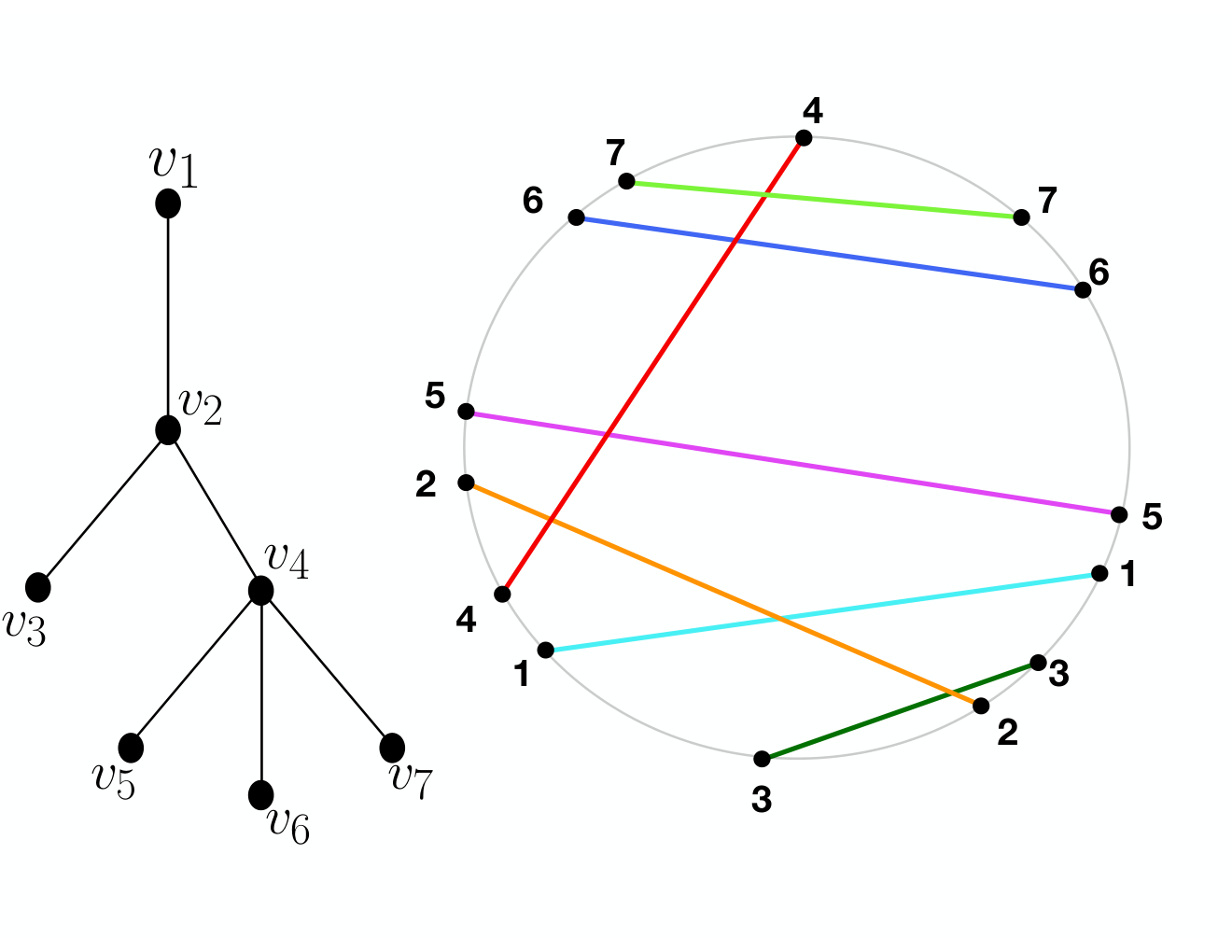
This completes the proof that any set $S$ of $2n$ points in convex position in the plane have a partition whose nerve is isomorphic to any given tree $T_{n}$. ∎

Let $\bar{S}$ be an arbitrary finite set of points in $\mathbb{R}^{d}$, such that $S\subset\bar{S}$. We begin by assuming that the “color partition function” $\mathcal{C}:S\to[n]$ is the one given in Theorem 4. It yields a partition $\mathcal{P}$ of $S$ with nerve $\mathcal{N}(\mathcal{P})$ isomorphic to $T_{n}$ and $n$ is the last color added. Recall that we denoted by $v_{r}$ the node in $T_{n-1}$ such that $\{v_{n},v_{r}\}$ is the leaf of $T_{n}$ in which we added $v_{n}$.

The extension of $\mathcal{P}$ of $S$ will be given through induction on $n$, by a “color partition function” $\bar{\mathcal{C}_{n}}:\bar{S}\to[n]$ as follows:

Let $S_{j}$ denote the set of points in $S$ of color $v_{j}$, or $j$ for simplicity. Consider the line $L_{n}$ through $S_{n}$ (it is given by points $\mathcal{S}_{2}$ and $\mathcal{S}_{2n}$ in Theorem 4), and recall that this line leaves only one element of $S_{r}$ in one side, say $L_{n}^{+}$, and the rest of the points of $S$ in the other side $L_{n}^{-}$. We define $\bar{\mathcal{C}}:\bar{S}\to[n]$ as follows: $\bar{\mathcal{C}_{n}}(\boldsymbol{x})=\bar{\mathcal{C}}_{n-1}(\boldsymbol{x})\text{\ when \ }\boldsymbol{x}\in L_{n}^{-}$, $\bar{\mathcal{C}_{n}}(\boldsymbol{x})=r\text{\ when \ }\boldsymbol{x}\in\conv(S_{r})$, and, finally, $\bar{\mathcal{C}_{n}}(\boldsymbol{x})=n\text{\ when \ }\boldsymbol{x}\in\cl(L_{n})^{+}\text{\ but \ }\boldsymbol{x}\notin\conv(S_{r}).$ Here $\cl(L_{n})^{+}$ denotes the closed half-plane at the right of $L_{n}$.

Observe that, by the induction process, the intersection pattern of $\bar{S}_{1},\dots\bar{S}_{n-1}$ are the same in ${L_{n}}^{-}$ by construction. Furthermore, $\cl(L_{n})^{+}$ does not intersect any other element in the partition, so no new intersections occur. ∎

Let $C_{m}(d)$ be an ordered cyclic $d$-polytope, with $m$ vertices and assume as before $S:=\{\boldsymbol{x}_{1},\boldsymbol{x}_{2},\dots\boldsymbol{x}_{m}\}$ along the curve. As in the case of the plane, the proof will be given by induction on $n$ the number of nodes of the tree $T_{n}$.

If $n=1$, again there is nothing to prove. If $n=2$, the only tree with two vertices is $K_{2}$. Then by Radon’s theorem, any set of $d+2$ points in $S$ can be partitioned in $S=S_{1}\cup S_{2}$ with $2\leq|S_{i}|\leq d$ for $i\in\{1,2\}$ and intersection graph $K_{2}$, see Figure 6 on the left.

For the induction step, suppose $T_{n}$ was obtained from $T_{n-1}$ by adding the node $v_{n}$ to a node $v_{r}\in T_{n-1}$ such that $\{v_{n},v_{r}\}$ is a leaf of $T_{n}$, and assume that $T_{n-1}$ is the nerve of some set $\mathcal{N}(\mathcal{P}^{\prime})$ where the set $S^{\prime}$ are the vertices of the ordered cyclic polytope with exactly $(n-1)(d+1)-d$ vertices in $\mathbb{R}^{d}$ and $\mathcal{P}^{\prime}=\{S^{\prime}_{1},S^{\prime}_{2},\dots,S^{\prime}_{n-1}\}$ are the color classes with color $1,2,\dots n-1$ respectively, via a “coloring function” $\mathcal{C}^{\prime}:S^{\prime}\to[n-1]$.

Let $k$ the maximum number in $[n]$ such that $\boldsymbol{x}_{k}$ is in $S^{\prime}_{r}$. Next in $C_{m}(d)$ consider the subpolytope $Q$ of $(n-1)(d+1)-d$ vertices, obtained as the convex hull $\conv(\boldsymbol{x}_{1},\boldsymbol{x}_{2},\dots,\boldsymbol{x}_{k},\boldsymbol{x}_{k+d+2},\dots\boldsymbol{x}_{m})$, and $R$ is the polytope consisting of the convex hull of the complement of $Q$ and $\boldsymbol{x}_{k}$, thus $R=\conv(\{\boldsymbol{x}_{k},\boldsymbol{x}_{k+1},\dots,\boldsymbol{x}_{k+d+1}\})$. Note both $Q$ and $R$ are ordered cyclic polytopes and $Q\cap R=\{\boldsymbol{x}_{k}\}$. Thus by the induction hypothesis there exists a partition of the vertices of $Q$ into $n-1$ color classes whose nerve is isomorphic to $T_{n-1}$ as before. Next, by Radon’s Lemma there exists a partition into two color classes $A$ and $B$ of the $d+2$ vertices of $R$.

Say $\boldsymbol{x}_{k}\in A$, then define a “coloring function” $\mathcal{C}:S\to[n]$ in the following way: $\mathcal{C}(\boldsymbol{x})=\mathcal{C}^{\prime}(\boldsymbol{x})$ if $\boldsymbol{x}$ is a vertex of $Q$, $\mathcal{C}(\boldsymbol{x})=r$ if $\boldsymbol{x}\in A$, and, finally, $\mathcal{C}(\boldsymbol{x})=n$ if $\boldsymbol{x}\in B$. That is $S_{n}\cap S_{r}\not=\emptyset$ and no further intersections occur. By the construction the parts of $\mathcal{P}$ consist of the $n$ color classes determined by the coloring $\mathcal{C}$. The nerve $\mathcal{N}(\mathcal{P})$ is isomorphic to $T_{n}$. ∎

Let $\bar{S}$ be an arbitrary finite set of points in $\mathbb{R}^{d}$, such that $S\subset\bar{S}$. Let $S_{j}$ denote the set of points in $S$ of color $v_{j}$, or $j$ for simplicity. Let us begin by assuming that the “color partition function” $\mathcal{C}:S\to[n]$, given in Theorem 5, yields a partition $\mathcal{P}$ of $S$ with nerve $\mathcal{N}(\mathcal{P})$ isomorphic to $T_{n}$. The extension of $\mathcal{P}$ of $S$ will be given by induction on the number of nodes $n$.

To begin observe that polytopes $Q$ and $R$ defined in Theorem 5 satisfy that $Q\cap R=\{\boldsymbol{x}_{k}\}$ so $(Q\setminus\{\boldsymbol{x}_{k}\})\cap(R\setminus\{\boldsymbol{x}_{k}\})=\emptyset$. Therefore, there exists a $(d-1)$-hyperplane $H$ that separates these two sets and leaves points of color $r$ in both sides of the hyperplane. Furthermore, $R$ is completely contained in the closure of one of the sides of this hyperplane, say $H_{n}^{-}$. The “color partition function” $\bar{\mathcal{C}_{n}}:\bar{S}\to[n]$ is given as follows:

$\bar{\mathcal{C}_{n}}(\boldsymbol{x})=\bar{\mathcal{C}}_{n-1}(\boldsymbol{x})\text{\ if \ }\boldsymbol{x}\in H_{n}^{-}$, $\bar{\mathcal{C}_{n}}(\boldsymbol{x})=r\text{\ if \ }\boldsymbol{x}\in S_{r}$, and $\bar{\mathcal{C}_{n}}(\boldsymbol{x})=n\text{\ if \ }\boldsymbol{x}\in\cl(H_{n}^{+})\text{\ and \ }\boldsymbol{x}\notin S_{n}$.

As before $\cl(H_{n}^{+})$ is the closed half-hyperplane containing only points in $R$ of color $n$ and color $r$.

Observe that by the induction process the intersection pattern of $\bar{S}_{1},\dots\bar{S}_{n-1}$ are the same in ${H_{n}}^{-}$ by construction, and $\cl(H_{n}^{+})\cap S_{r}\not=\emptyset$ yields the leaf $\{v_{r},v_{n}\}$. Furthermore $S_{n}\subset\cl(H_{n}^{+})$ does not intersect any other elements in the partition since they are contained in $H_{n}^{-}$, so no further intersections occur.

∎

Suppose that $\bar{S}$ is a set of at least $nd+n+4d$ points in general position in $\mathbb{R}^{d}$. We start by projecting the points onto a generic $2$-plane $H$ where we can assume, without loss of generality, that the points of $\bar{S}$ have distinct projections onto it. Let $S$ be the projection of $\bar{S}$, now planar points.

Now we will use the the subdivision $C^{\prime}$, whose existence is guaranteed by Lemma 5, to find our desired partition of the data points whose partition nerve is an $n$-cycle.

We construct a partition one sector at a time. In the first step, we notice that one of the $n$ sectors, say $Q_{1}$, has at least $d+2$ points by the pigeonhole principle.
Use Radon’s Lemma to partition the points in $Q_{1}$ into two sets $S_{1}$ and $S_{2}$ so that the convex hulls of $S_{1}$ and $S_{2}$ intersect.

In the second step, we denote the slice counterclockwise to $Q_{1}$ as $Q_{2}$.
By Radon’s Lemma, any point $\boldsymbol{x}_{2}$ in $S_{2}$ from step 1, combined with the (at least) $d+1$ points in $Q_{2}$ can be partitioned into two sets $S_{2}^{\prime}$ and $S_{3}$ so that the convex hulls of $S_{2}$ and $S_{3}$ intersect. Without loss of generality we can assume that $\boldsymbol{x}_{2}\in S_{2}^{\prime}$, and then set $S_{2}=S_{2}\cup S_{2}^{\prime}$. In step $k$, where $3\leq k\leq n-1$, we continue in the same way. We denote the slice counterclockwise to $Q_{k-1}$ as $Q_{k}$.
By Radon’s Lemma, any point $\boldsymbol{x}_{k}$ in $S_{k}$ from step $(k-1)$, combined with the (at least) $d+1$ points in $Q_{k+1}$ can be partitioned into two sets $S_{k}^{\prime}$ and $S_{k+1}$ so that the convex hulls of $S_{k}^{\prime}$ and $S_{k+1}$ intersect. Without loss of generality we can assume that $\boldsymbol{x}_{k-1}\in S_{k-1}^{\prime}$, and then set $S_{k}=S_{k}\cup S_{k}^{\prime}$. Finally, in step $n-1$ we set $S_{1}=S_{1}\cup S_{n}$.

We claim that the nerve of the resulting partition $\mathcal{P}=\{S_{1},S_{2},\dots,S_{n}\}$ is the $n$-cycle.
This is a consequence of two facts: We used Radon’s Lemma to guarantee that any two subsets appearing in the same sector have intersecting convex hulls. Each subset appears in at most two sectors, and since two adjacent sectors have a combined angle of at most $\pi$ radians there is a line separating any two subsets that do not appear in the same sector. Thus we have that $\conv(S_{i})\cap\conv(S_{j})\neq\emptyset$ if and only if there is some sector containing points from both $S_{i}$ and $S_{j}$. If we let ${\bf v}_{i}$ denote the vertex of the nerve corresponding to subset $S_{i}$, we see that the edges of $\mathcal{N}(\mathcal{P})$ consist precisely of $({\bf v}_{n},\bf{v}_{1})$ and $(\bf{v}_{i},\bf{v}_{i+1})$ where $i\in[n-1]$. This completes the proof. ∎

We prove this by induction on $n$. For $n=1$, the partition of one point to get $St_{1}$ is obvious. Now assume the result is true for some $n$. We need to show that any $(d+1)n+1$ points can be partitioned with partition nerve $St_{n+1}$. Let $M=(n-1)(d+1)+1$. By induction hypothesis, the subset $\{\boldsymbol{x}_{1},\dots,\boldsymbol{x}_{M}\}\subset S$ admits a partition $\mathcal{P}=\{A_{1},\ldots,A_{n}\}$ with $\mathcal{N}(\mathcal{P})\simeq St_{n}$. Without loss of generality, assume that $A_{1}$ is the central vertex of the star graph. Let $\boldsymbol{x}\in S$ be some point in $A_{1}$. By Radon’s lemma, there is a way to partition the $d+2$ points $\boldsymbol{x},\boldsymbol{x}_{M},\boldsymbol{x}_{M+1},\dots\boldsymbol{x}_{M+d+1}$ into two sets $X,Y$ with $\conv(X)\cap\conv(Y)\neq\emptyset$, and we can assume that $\boldsymbol{x}\in X$. The set $Y$ intersects $A_{1}\cup X$ but does not intersect any of $A_{i}$, $2\leq i\leq n$, because every point in $Y$ has larger first coordinate than any point in $A_{i}$. Then we see $\{A_{1}\cup X,A_{2},\ldots,A_{n},Y\}$ is a partition which will induce the star graph $St_{n}$. ∎

Now we prove that for every caterpillar tree $T_{n}$ with at most $n$ nodes, every set $S$ with at least $(d+1)(n-1)+1$ points in $\mathbb{R}^{d}$ admits a partition $\mathcal{P}$ with $\mathcal{N}(\mathcal{P})\simeq T_{n}$. An illustration of the partition constructed in the proof is given in the Figure 8. The proof is by induction on the length of the central path in $T_{n}$, which we will denote by $m$. The induction hypothesis says that for every $m\in\mathbb{N}$ and any caterpillar tree $T_{n}$ with $n$ vertices and a central path of length $m$ the following two statements hold:
(1) Every set $S$ of $(d+1)(n-1)+1$ points in $\mathbb{R}^{d}$ admits a partition $\mathcal{P}$ with $\mathcal{N}(\mathcal{P})\simeq T_{n}$
(2) Denote by $v$ the last vertex of the central path, and denote by $St_{k+1}$ the star subgraph induced by $v$ and its $k$ neighbors. Then the subsets in $\mathcal{P}$ corresponding to vertices in $St_{k+1}$ are comprised of the $(d+1)k+d+1$ points in $S$ with largest first coordinate.

If the length of the central path is one, both parts of the induction hypothesis follow by applying Lemma 6. Assume the result holds if the central path is of length $m$. We consider caterpillar graphs which have central paths of length $m+1$. Let $G$ be such a graph with $n$ vertices. We consider the endpoint of the path $v_{m+1}$ and the vertex prior $v_{m}$. If we consider the subgraph of $G$ consisting of the path $v_{1},\ldots,v_{m}$ and all vertices adjacent to it except $v_{m+1}$, this is a caterpillar graph with a path of length $m$. Let $p$ denote the number of vertices of this graph. By induction hypothesis, we can represent this graph using the $(d+1)(p-1)+1$ points $\boldsymbol{x}_{1},\dots,\boldsymbol{x}_{(d+1)(p-1)+1}$. We will have the partition $\{A_{1},\dots,A_{p}\}$ where we take $A_{1}$ to be the set corresponding to $v_{m}$. Then take a point $\boldsymbol{x}\in A_{1}$ and the next $d+1$ points $\boldsymbol{x}_{(d+1)(p_{1})+2},\dots,\boldsymbol{x}_{(d+1)(p_{1})+d+2}$ to have a Radon partition $X,Y$ with $\boldsymbol{x}\in X$. Our new partition will be $\{A_{1}\cup X,A_{2},\ldots,A_{p},Y\}$. $Y$ will correspond to the vertex $v_{m+1}$ and will not intersect any of the other sets due to having larger first coordinate. In addition, $A_{1}\cup X$ will not intersect any new sets by how we have arranged the points due to the induction hypothesis. Now as in the proof of the lemma, we can add new sets by considering $(d+1)$ points in iteration for each of the other vertices adjacent to $v_{m+1}$. Since there were $n-p$ vertices and we used $(d+1)$ points for each, in total we used $(d+1)(n-1)+1+(d+1)(n-p)=(d+1)(n-1)+1$ points. This is the desired number.

Thus we have proved the induction hypothesis. To complete the proof of the theorem, we note that if we have more than $(d+1)(n-1)+1$ points, we can apply the induction hypothesis to find the desired partition of the $(d+1)(n-1)+1$ points $\boldsymbol{x}_{1},\boldsymbol{x}_{2},\dots\boldsymbol{x}_{(d+1)(n-1)+1}$, then add any remaining points to the subset corresponding to the endpoint of the central path in the caterpillar graph. ∎

Suppose we have points $\boldsymbol{p}_{1}$ and $\boldsymbol{p}_{2}$ as hypothesized and partition the remaining points into $A$ and $B$. Let $L$ be the line between $\boldsymbol{p}_{1}$ and $\boldsymbol{p}_{2}$. To pair off the points, we consider the vertices of $conv(A\cup B)$. Since $L$ separates the points of $A$ and $B$, we must have that there are a pair of adjacent vertices of $conv(A\cup B)$ such that one, $\boldsymbol{a}_{1}$, is a member of $A$ and the other $\boldsymbol{b}_{1}$, a member of $B$. The segment between this pair cannot intersect the segment between any other pair of points as this segment forms the boundary of the convex hull. We pair off these two points and then consider $conv(A\setminus\{\boldsymbol{a}_{1}\}\cup B\setminus\{\boldsymbol{b}_{1}\})$. We see that $L$ separates $A\setminus\{\boldsymbol{a}_{1}\}$ and $B\setminus\{\boldsymbol{b}_{1}\}$, so we can repeat this argument to pair off $\boldsymbol{a}_{2}$ and $\boldsymbol{b}_{2}$. Continuing in this fashion until we have paired off all the elements, we will have a pairing $(\boldsymbol{a}_{1},\boldsymbol{b}_{1}),(\boldsymbol{a}_{2},\boldsymbol{b}_{2}),\ldots,(\boldsymbol{a}_{n},\boldsymbol{b}_{n})$ where $L_{\boldsymbol{a}_{i}\boldsymbol{b}_{i}}$ does not intersect $L_{\boldsymbol{a}_{j}\boldsymbol{b}_{j}}$ for $i\neq j$. ∎

References

- [AAK02] O. Aichholzer, F. Aurenhammer, and H. Krasser, Enumerating order types for small point sets with applications, Order 19 (2002), no. 3, 265–281.
- [BLVS+93] A. Björner, M. Las Vergnas, B. Sturmfels, N. White, and G. M. Ziegler, Oriented matroids, Encyclopedia of Mathematics and its Applications, vol. 46, Cambridge University Press, Cambridge, 1993. MR 1226888
- [BS17] I. Bárány and P. Soberón, Tverberg’s theorem is 50 years old: a survey, ArXiv e-prints (2017).
- [CD00] R. Cordovil and P. Duchet, Cyclic polytopes and oriented matroids, European Journal of Combinatorics 21 (2000), no. 1, 49 – 64.
- [CFS10] D. Conlon, J. Fox, and B. Sudakov, Hypergraph Ramsey numbers, J. Amer. Math. Soc. 23 (2010), no. 1, 247–266. MR 2552253
- [Eck93] J. Eckhoff, Extremal interval graphs, J. Graph Theory 17 (1993), no. 1, 117–127. MR 1201250
- [ES35] P. Erdös and G. Szekeres, A combinatorial problem in geometry, Compositio Math. 2 (1935), 463–470. MR 1556929
- [Gr67] B. Grünbaum, Convex polytopes, With the cooperation of V. Klee, M. A. Perles and G. C. Shephard. Pure and Applied Mathematics, Vol. 16, Interscience Publishers John Wiley & Sons, Inc., New York, 1967. MR 0226496
- [LB62] C. Lekkerkerker and J. Boland, Representation of a finite graph by a set of intervals on the real line, Fundamenta Mathematicae 51 (1962), no. 1, 45–64 (eng).
- [Mat02] J. Matoušek, Lectures on discrete geometry, Graduate Texts in Mathematics, vol. 212, Springer-Verlag, New York, 2002.
- [MS16] W. Morris and V. Soltan, The Erdös-Szekeres problem, Open problems in mathematics, Springer, [Cham], 2016, pp. 351–375. MR 3526941
- [Pm85] G. Ya. Perel′ man, Realization of abstract -skeletons as -skeletons of intersections of convex polyhedra in , Geometric questions in the theory of functions and sets, Kalinin. Gos. Univ., Kalinin, 1985, pp. 129–131. MR 829936
- [PS16] M.A. Perles and M. Sigron, Some variations on Tverberg’s theorem, Israel Journal of Mathematics 216 (2016), no. 2, 957–972.
- [Rea79] J. R. Reay, Several generalizations of Tverberg’s theorem, Israel Journal of Mathematics 34 (1979), no. 3, 238–244.
- [RGZ97] J. Richter-Gebert and G. M. Ziegler, Oriented matroids, Handbook of discrete and computational geometry, CRC Press Ser. Discrete Math. Appl., CRC, Boca Raton, FL, 1997, pp. 111–132. MR 1730162
- [Rou09] J.P. Roudneff, New cases of Reay’s conjecture on partitions of points into simplices with k-dimensional intersection, European Journal of Combinatorics 30 (2009), no. 8, 1919 – 1943, Combinatorial Geometries and Applications: Oriented Matroids and Matroids.
- [Stu87] B. Sturmfels, Cyclic polytopes and -order curves, Geom. Dedicata 24 (1987), no. 1, 103–107. MR 904552
- [Suk17] A. Suk, On the Erdös-Szekeres convex polygon problem, J. Amer. Math. Soc. 30 (2017), no. 4, 1047–1053. MR 3671936
- [Tan11] M. Tancer, -representability of simplicial complexes of fixed dimension, J. Comput. Geom. 2 (2011), no. 1, 183–188. MR 2855919
- [Tan13] by same author, Intersection patterns of convex sets via simplicial complexes: a survey, Thirty essays on geometric graph theory, Springer, New York, 2013, pp. 521–540. MR 3205172
- [Tve66] H. Tverberg, A generalization of Radon’s theorem, J. London Math. Soc. 41 (1966), no. 1, 123–128.
- [Weg67] G. Wegner, Eigenschaften der nerven homologisch-einfacher familien im , Ph.D. thesis, Georg-August-Universita̋t Gőttingen, 1967.
5. Appendix: Proofs of auxiliary lemmas
In this appendix we include proofs of some supplementary lemmas mentioned in the introduction.
Proof of Lemma 1.
Suppose by contradiction . Let be a set of points in convex position with . By the pigeonhole principle, if we partition into disjoint subsets, there must be at least one subset that is a singleton . Since is connected, the node corresponding to the singleton is connected, by an edge, to at least one other node, implying that is in the convex hull of another subset. However, this is a contradiction as the points are in convex position. ∎
Proof of Lemma 2.
To show that it suffices to show that if and only if for all . Suppose . Then they contain respectively and which are an inclusion minimal Radon partition of . Since is an order-preserving bijection, is an isomorphism between oriented matroids (see, for instance [RGZ97]) determined by and . The minimal Radon partitions in correspond to the circuits of the oriented matroids and therefore are preserved under . Thus . The reverse implication is shown by the reasoning applied to . ∎
As we mentioned in the Introduction, the graph in Figure 13 is -partition induced (in particular by the partitioned point set in Figure 13), but not -Tverberg, as implied by the following lemma:
Lemma 8.
Suppose is any set of points in convex position in . Then the graph in Figure 13 is not partition induced on .
Proof.
We note that since is a triangle free graph, it suffices to show that it is not the intersection graph of any partition of points in convex position. We argue by contradiction. Suppose that there is a set of points in convex position partitioned so that they have the graph above as their intersection graph. By Lemma 2 we may assume the points are arranged on the boundary of a disc . Denote the convex hull of the points corresponding to each node by region . In the rest of the proof of Lemma 8, we will rely on the following.
Claim 6.
Consider the independent set of nodes in Figure 13. Up to exchanging their labels (note that the graph is symmetric about ), there are two possible arrangements of the regions ,, and , pictured in Figures 6 and 6.
![[Uncaptioned image]](1808.00551v1/convexcase1.PNG)
![[Uncaptioned image]](1808.00551v1/convexcase2.PNG)
Proof of the claim.
The region has two connected components. If regions and lie in different connected components of , then regions and must be arranged as in Figure 6. Otherwise, and lie in the same connected component, say , of . If we walk clockwise around the boundary of , we can only alternate twice between being in regions and , reducing to the two possibilities shown. ∎
By the claim, we see that and must be arranged (up to symmetry) as in one of the two cases pictured above. If they are arranged as in Figure 6, note that regions and both intersect regions and . In that case it is easy to see that regions and must intersect, which is a contradiction.
If the regions are arranged as in Figure 6, consider that regions and . Note that region intersects regions . Also, region is disjoint from all the regions through , while intersecting region . Similarly, region is disjoint from all the regions through except . Also region is disjoint from all the regions through except . Considering the two cases: lie in the same connected component of , or lie in different connected components of , it is easy to see that, in both cases, and must be arranged as and are in Figure 6. Then are disjoint but both intersect and , which is a contradiction by the argument above. Thus cannot be the nerve of a set of points in convex position. ∎