On two types of Heegaard diagram used in knot Floer homology
Abstract.
In this brief note, we give an explicit sequence of Heegaard moves interpolating between local versions of the Kauffman-states Heegaard diagram and the planar Heegaard diagram used in knot Floer homology, and show how these local moves can be used to go between the global versions of the Heegaard diagrams.
1. Introduction
Knot Floer homology [17, 24] is a powerful modern invariant for knots and links in -manifolds. It is related to the Heegaard Floer invariants for - and -manifolds defined by Ozsváth–Szabó [18, 19], it categorifies the Alexander polynomial, and it exactly detects many important topological properties of knots that are only bounded or restricted by the Alexander polynomial.
To define the knot Floer homology of a knot or link , one must first choose a Heegaard diagram representing ; in general this can be a multi-pointed diagram as in [12, Section 2]. From the diagram, one gets a graded free abelian group with a natural basis; after making additional analytic choies, one gets a differential on this group such that the homology of the resulting complex (up to isomorphism, and after correcting for tensor factors that result from having multiple basepoints) is an invariant of .
There are always infinitely many diagrams representing any knot or link. In order to study the algebraic properties of knot Floer homology, various systematic procedures for constructing multi-pointed Heegaard diagrams from knot projections have been considered.
One such procedure, introduced in [16], constructs a two-pointed Heegaard diagram from a projection of a knot or link in . Generators of the chain complex associated to this diagram are in bijection with Kauffman states [5] of the projection. This family of Heegaard diagrams, the “Kauffman-states diagrams,” have recently provided [22, 23, 14, 15] the basis for a deep and sophisticated algebraic apparatus for knot Floer homology in the spirit of bordered Floer homology [6], raising hopes for new relationships between knot Floer homology and constructions in representation theory (see [8, 9]). This procedure was generalized by Ozsváth–Stipsicz–Szabó in [13] to define diagrams for singular as well as nonsingular crossings.
Another procedure for constructing multi-pointed Heegaard diagrams from knot projections yields the “planar” Heegaard diagrams. These diagrams were first defined for fully singular link diagrams in [13, Section 5] and generalized for all link diagrams in [21, Figure 12] (the exact version we consider was defined in [11]). The planar diagrams seem especially suited for studying the relationship between Heegaard Floer homology and HOMFLY-PT homology; see [2, 3, 4].
Given the recent results about knot Floer homology based on both types of diagrams, it is natural to ask whether the two procedures mentioned above are related. In principle, any two multi-pointed Heegaard diagrams representing the same link can be related by a sequence of Heegaard moves, i.e. isotopies, stabilizations (of two types), destabilizations, and handleslides. The proof of this fact relies on Morse theory and is non-constructive; it is desirable to have a constructive proof that the specific diagrams in question are related by Heegaard moves.
Indeed, this question was addressed for fully singular link projections in [21, proof of Lemma 3.7]. Ozsváth–Szabó construct a sequence of Heegaard moves transforming the Kauffman-states diagram into the planar diagram for a fully singular link projection. Besides the limitation to singular projections, however, another potentially undesirable feature of this construction is that it treats crossings differently depending on the position of their edges in an ordering on all the edges of the link projection.
In this note, given a link projection that may have nonsingular as well as singular crossings, we construct an explicit sequence of Heegaard moves which transform the Kauffman-states diagram of the projection into the planar diagram of the projection. Our construction is more local in character than the one given in [21, proof of Lemma 3.7] for fully singular projections; all crossings (whether singular or nonsingular) are treated similarly and independently of the rest of the diagram. Our main result may be summarized as follows:
Theorem 1.1.
The sequence of moves outlined in Construction 4.3 below transforms the Kauffman-states diagram of a (possibly singular) link projection into the planar diagram of the projection.
We use a version of the Kauffman-states diagram with “ladybugs” added as in [10]; see Section 2.3 below. Ladybugs are often useful when working with the Kauffman-states diagram; see for example [1]. The diagrams with ladybugs can be transformed into the original diagrams using Heegaard moves, including index zero/three stabilizations, discussed in Section 2.5 below. We review one way of doing this in Example 2.9.
Construction 4.3 will start by modifying a stabilized version of the Kauffman states diagram near each crossing, before performing additional moves that do not depend on whether the crossings are positive, negative, or singularized. To deal with the local constructions, we will introduce some basic definitions for Heegaard diagrams with boundary in Section 2. The local constructions will be given in Section 3; they will be patched together into moves relating the global Heegaard diagrams in Section 4.
1.1. Motivation
One motivation for this work is to understand the planar diagram, and eventually its associated Heegaard Floer invariants, locally using the methods of bordered Floer homology. As a prerequisite for this algebraic setup, one needs to choose a decomposition of the Heegaard diagram into pieces satisfying certain properties. Combinatorial details of the pieces determine how the algebraic invariants work and how easy it is to define them. There are various possible decompositions of the planar diagram to which one could apply the ideas of bordered Floer homology; in this paper we study a decomposition related to one which has already been used for bordered Floer homology in [22, 23].
In particular, applying the bordered-Floer methods used in [22, 23], one should be able to define a bimodule over the algebras from [22, 23] associated to each “row” of a Heegaard diagram like the one shown in the top-right corner of Figure 47. One would then expect homotopy equivalences between these bimodules and the bimodules defined for nonsingular crossings in [22] or [23] (depending on the chosen algebraic setup) and for singular crossings in [7] (in preparation); however, as currently planned, only local bimodules for a singular crossing between two strands will be defined in [7].
One reason why the hypothetical bimodules of the previous paragraph would be interesting is that they could be used to give a local formulation of the singular skein exact triangle and cube of resolutions in knot Floer homology [21, 11]. The construction of this exact triangle uses the planar diagrams for a nonsingular crossing, its singularization, and its resolution. The corresponding bimodules should satisfy a mapping-cone relation. Constructing these bimodules and proving such a relationship could lead to local versions of results of Dowlin [2, 3, 4] and further progress in the relationship between knot Floer homology and HOMFLY-PT homology.
1.2. Acknowledgments
I would like to thank Zoltán Szabó for introducing me to the Heegaard diagrams behind [22, 23], in particular the stabilizations which proved essential in the constructions of this paper. I would also like to thank Nathan Dowlin, Aaron Lauda, Robert Lipshitz, Ciprian Manolescu, and Ina Petkova for useful conversations. This work was supported by the National Science Foundation under Grant No. DMS-1502686.
2. Preliminaries
2.1. Partial Heegaard diagrams
Since we do not discuss algebraic invariants in this paper, the following (overly permissive in general) definition will suffice for our local constructions.
Definition 2.1.
A partial Heegaard diagram is a compact oriented surface with boundary, equipped with two finite collections of circles (the and circles) smoothly embedded in , two finite collections of compact intervals (the and arcs) smoothly embedded in , and a collection of basepoints labelled either or which does not intersect or the or circles or arcs, such that:
- •
The endpoints of the and arcs lie in , and these arcs intersect transversely
- •
There are no intersections between an arc or circle and another arc or circle, and similarly for arcs and circles
- •
Any intersections between and arcs or circles are transverse and occur in .
We will always consider partial Heegaard diagrams up to boundary-preserving isotopies that do not change any of the combinatorial properties of the basepoints or and arcs and circles. As we will see below, we are even more interested in a coarser equivalence relation on partial Heegaard diagrams that (in particular) allows more general types of isotopy.
We briefly review how Heegaard diagrams are used to represent -manifolds and links. Suppose that and that adding -dimensional -handles to along the circles and yields a -manifold with boundary (in particular, the number of circles and the number of circles must each equal the genus of ). In this case, we may form a closed -manifold by filling in the boundary components with copies of . The orientation on allows us to specify an orientation on . The Heegaard diagram (disregarding the basepoint data) is said to represent the closed oriented -manifold . The Kauffman states and planar diagrams considered in this paper represent .
For a Heegaard diagram representing a closed -manifold , assume that each connected component of the complement of the circles in contains exactly one basepoint and one basepoint, and that the same is true for the complement of the circles. If we first remove a small disk around each basepoint of , thicken and attach handles as above, and omit adding copies of , the resulting -manifold is the complement of a link in the closed -manifold represented by . From the types ( and ) of the basepoints, we can give an orientation (see e.g. Figure 3). We say that represents . This definition can be generalized for singular links. The Kauffman states and planar diagrams associated to a projection of an oriented (and possibly singular) link represent .
Remark 2.2.
More generally, if has boundary but no or arcs, one can form a sutured -manifold from by performing a similar thickening-and-handle-addition procedure. When represents as above and we construct a Heegaard diagram from by cutting out a small disk around every basepoint, then has no or arcs, so it represents a sutured manifold. This manifold is the link complement in which each component of the boundary has been given a meridional suture for each and basepoint corresponding to the component.
2.2. Gluing
Suppose and are partial Heegaard diagrams. Let and be sets of connected components of and respectively, with elements each, and suppose that for each we are given a diffeomorphism from to restricting to a bijection between the sets of endpoints of and arcs intersecting and . We can form a new partial Heegaard diagram by gluing each component to via the given diffeomorphisms; we are omitting some details here, but these are not worrisome because we are only dealing with circles and surfaces.
2.3. The Kauffman-states diagram
Let be a (generic) projection of a link in onto the plane ; for simplicity, assume that has a unique global minimum point in this plane. Also choose a finite set of points on , away from the crossings and the global minimum. When we are given this data, we will call a marked projection.
Assume that every component of contains either the global minimum or at least one . We will define the Kauffman-states Heegaard diagram for with the distinguished point placed at the global minimum and with ladybugs added at the points . The choice of the (given the above restriction) is irrelevant up to Heegaard moves, which will be discussed in Section 2.5 below (see Example 2.9 in particular).

Example 2.3.
The Kauffman-states Heegaard diagrams for marked projections of the trefoil and Hopf link are shown in Figure 1. The global minimum of each projection is shown with a dot; the marked points are shown with dashes.

Example 2.4.
The Kauffman-states Heegaard diagram for a different marked projection of the trefoil, with more marked points (and thus more ladybugs), is shown in Figure 2.

In general, we can define the Kauffman states Heegaard diagram by gluing it together from the partial Heegaard diagrams shown in Figure 3. When an arc in one of the local pieces would be adjacent to the unbounded region of the projection in the glued-together diagram, it should be omitted from the local piece.

2.4. The planar diagram
We will also define the planar diagram from [21, Section 4] of a link projection . This diagram is called planar because it has , unlike the Kauffman-states diagram.

Example 2.5.
The planar Heegaard diagrams for projections of the trefoil and Hopf link are shown in Figure 5. Each picture should be interpreted as being embedded in a -sphere which we will not draw.


As with the Kauffman-states diagram, we can define the planar diagram by gluing together partial Heegaard diagrams. The partial diagrams for singular and nonsingular crossings are shown in Figure 6. To form the full planar diagram, one first glues the diagram for each crossing into an “outside” diagram depending on the projection, as in Figure 7. Then one removes the circle corresponding to the distinguished edge (the global minimum) and its corresponding small circle.

Remark 2.6.
Often one works with a smaller variant of the planar diagram, shown for the trefoil in Figure 8. This smaller diagram can be obtained from the one we use by a series of handleslides and index zero/three stabilizations.
2.5. Heegaard moves
We now discuss certain modifications one can perform to a partial Heegaard diagram, called Heegaard moves.
Remark 2.7.
If a Heegaard diagram represents a closed -manifold or a link , this fact is invariant under performing Heegaard moves on the diagram. This is not quite true in the sutured setting of Remark 2.2; the index zero/three stabilization described below does not leave the sutured -manifold unchanged, but it modifies the sutured structure of the manifold in a predictable way.

Definition 2.8.
For us, a Heegaard move is a modification of a partial Heegaard diagram in any of the following ways. A variation of this set of moves can be found in [20, Proposition 3.3]; for the specific form of the index zero/three stabilization given below, see [12, Lemma 2.4 and Figure 5]. The terminology for stabilizations comes from Morse theory.
- •
First, one is allowed to isotope the Heegaard diagram as in the top row of Figure 9. These isotopies are allowed to change the combinatorial properties of the and curves (e.g. their number of intersections), but the boundary of the Heegaard diagram must remain fixed and curves are not allowed to move past basepoints.
- •
Second, one is allowed to perform an index one/two stabilization as in the second row of Figure 9, or to undo such a stabilization. The analogous stabilization with the roles of the and curves reversed is also allowed. Note that the given form of the index one/two stabilization can be obtained from the simpler form described e.g. in [20, Proposition 3.3] by using handleslides; we find it convenient to work with the given form.
- •
Third, one is allowed to perform an index zero/three stabilization as in the third and fourth rows of Figure 9, or to undo such a stabilization.
- •
Finally, one is allowed to handleslide an circle over an circle, or a circle over a circle, as in the fifth row of Figure 9.


Example 2.9.
In the case of the Kauffman-states diagram for the trefoil from Figure 1 above, we show how to implement the addition of a ladybug using Heegaard moves in Figure 10. The first step is an index zero/three stabilization. The second step is a handleslide of a circle; at this point we have produced a ladybug near the global minimum of the projection.
The remaining steps show how to move a ladybug past a (nonsingular) crossing. The third step is a combinatorics-preserving isotopy to make things easier to see. The fourth step is a handleslide of an circle, together with another combinatorics-preserving isotopy for simplification. The fifth step is a handleslide of a circle. The sixth and seventh step are isotopies that reduce the number of intersections between and circles.
Ladybug addition works like this in general if is nonsingular. To add a ladybug on a component of that does not contain the global minimum, we start with an index zero/three stabilization at a pre-existing ladybug on this component, as shown in Figure 11.
If has singular crossings, one can create ladybugs at either of the two incoming edges of a singular crossing, just as one does at the global minimum. These ladybugs can then be propagated backwards along , away from the singular crossing, until another singular crossing is reached which can create its own ladybugs. In this way, one can go from the Kauffman-states diagram without ladybugs to the Kauffman-states diagram for an arbitrary marking of the projection using the Heegaard moves of Definition 2.8.
Adding or removing ladybugs is the only construction in this paper requiring the link projection to be traversed in-line as in [21, proof of Lemma 3.7].
2.6. Gluing and Heegaard moves
The following fact will be useful in assembling our sequence of Heegaard moves from local pieces; in fact, our main justification for describing our construction as “local” is that this proposition is used repeatedly in Construction 4.3.
Proposition 2.10.
If and are partial Heegaard diagrams obtained from and by Heegaard moves, and we glue and to get as in Section 2.2, then we may also glue and to obtain a partial Heegaard diagram , and the sequences of Heegaard moves transforming and into and may be combined to transform into .
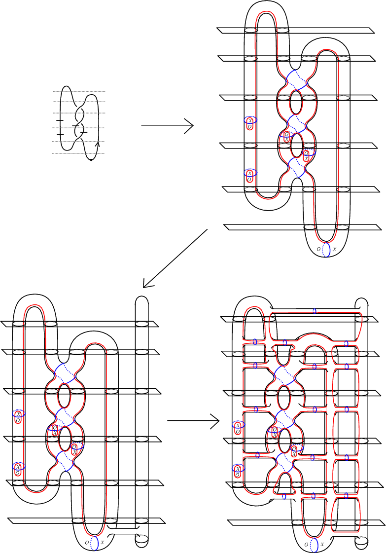
Example 2.11.
Let be a marked link projection; generically we may assume that can be written as a vertical concatenation of crossings (possibly singular), maximum points, and minimum points. Such a projection is shown in the top-left corner of Figure 12.
The Kauffman-states diagram of can be viewed as being glued together from partial diagrams as shown in the top-right corner of Figure 12. We stretch the Kauffman-states diagram of as shown in the bottom-left corner of Figure 12. Then, in the spirit of Ozsváth–Szabó’s recent work [22, 23], we perform a series of index one/two stabilizations (and handleslides of circles) to obtain the diagram in the bottom-right corner of Figure 12. These stabilizations are useful when treating the Kauffman-states diagram using bordered Floer homology; they will turn out to be important in our construction as well.
Remark 2.12.
Diagrams obtained by placing a stabilization point in a different position than the one shown in Figure 12 (e.g. below a crossing as opposed to above it) are related by handleslides of circles.


Example 2.13.
We can view the Kauffman-states diagram, in the version shown in the bottom-left corner of Figure 12, as glued together from the partial Heegaard diagrams shown in Figure 13. Furthermore, we can assemble each of the diagrams in Figure 13 from the partial Heegaard diagrams shown in Figure 14. Ladybugs are omitted for simplicity, but in general all pieces in Figure 14 are allowed to have ladybugs added.
2.7. Planar pieces

The following definition is motivated by the structure of the planar Heegaard diagram:
Definition 2.14.
A planar piece is a partial Heegaard diagram whose underlying surface is , with arcs intersecting the top part of and arcs intersecting the bottom part of , such that when the components of the complement of the arcs and circles in are alternatingly shaded and unshaded as shown in Figure 15, there exists no path from a basepoint to contained entirely in an unshaded region.
Example 2.15.

Remark 2.16.
If is a planar piece, then modifying as shown in the top two rows Figure 16 produces another planar piece. In general, one can add parallel arcs to the left of and parallel arcs to the right of and obtain another planar piece. If and are planar pieces with arcs intersecting the top of and the bottom of , then gluing and as at the bottom of Figure 16 produces another planar piece. Also note that endpoints of arcs can be rotated two-at-a-time from the bottom to the top of a planar piece.
3. Heegaard moves local to crossings
The goal of this section is to transform the partial Heegaard diagrams of Figure 14 into ones that can be understood using the planar pieces of Figure 6 using Heegaard moves.


To describe these moves, it is helpful to re-draw the diagrams of Figure 14 in a more planar way. Figure 17 shows an alternative view of the diagrams of Figure 14 (with a few handleslides done to make the diagrams look nicer; these come from moving the stabilization points as in Remark 2.12). All diagrams are assumed to be drawn on ; we will not draw these spheres to save space. Figure 18 shows how to go from one view to the other in one example.


We now add the ladybugs that we will need (these were assumed to be potentially present the whole time). Some of the diagrams from Figure 17 that get ladybugs are shown (along with two diagrams that get no ladybugs) in Figure 19. Nonsingular crossings can have four possible orientation patterns, and the and basepoints in the ladybugs depend on the orientation.
The rest of the diagrams that get ladybugs are shown in Figure 20, again with two diagrams that get no ladybugs. The diagrams in Figure 19 and Figure 20 are the ones we will transform using Construction 3.1.


The following construction transforms the diagrams of Figure 19 into the diagrams of Figure 21. The same steps apply to transform the diagrams of Figure 20 into the diagrams of Figure 22.
Construction 3.1.
Starting from the diagram at the left of Figure 23 (row 1, column 1 of Figure 19), handleslide the “diagonal” circle to get the second diagram of Figure 23. Handleslide an circle to get the third diagram of Figure 23. Wrap the rightmost circle around the back of to get the fourth diagram of Figure 23. Finally, perform several handleslides of this circle, as shown in the subsequent diagrams of Figure 23.


The diagrams in Figure 21 all have a special form. If is a planar piece with endpoints of arcs along the top of and endpoints of arcs along the bottom, we can form a new partial Heegaard diagram by gluing into the diagram shown in the top row of Figure 37. We get the diagrams in Figure 22 by gluing into the diagram shown on in the bottom row of Figure 37 instead. All the diagrams in Figure 21 can be obtained by applying this procedure to a planar piece from Figure 38; these pieces are the possible local pieces of the planar diagram when one does not mod out by rotation.


Remark 3.2.
When working with the cube of resolutions, there is a third variant of the planar diagram that appears for resolutions of crossings. This diagram is shown in Figure 39, along with the four ways to insert it into the top diagram of Figure 37 depending on orientations. Construction 3.1 can be modified to obtain these diagram from the Kauffman-states diagrams shown on the right of Figure 40. We show the required Heegaard moves in Figure 41; they are very similar to the ones appearing in Construction 3.1.
4. Global diagrams


Let be a planar piece with top endpoints and bottom endpoints. Let be the partial Heegaard diagram of Figure 42, with endpoints chosen so that it makes sense to glue into . Let denote the planar piece obtained by inserting parallel arcs at the left of and parallel arcs at the right of as in Remark 2.16. Finally, let denote the Heegaard diagram shown in Figure 43 with endpoints of arcs at the top and endpoints of arcs at the bottom. We will give a sequence of Heegaard moves transforming into .


Construction 4.1.
Starting from as shown in the top row of Figure 44, perform a sequence of handleslides on the curves on the left side of the diagram as shown in the subsequent rows of Figure 44. Next, do the same with the curves on the right side of the diagram, as shown in Figure 45.
From the diagram in the fourth row of Figure 45, wrap a circle around the back of , then handleslide it through as in the fifth row of Figure 45. The handleslide through is the crucial step; it is possible because was assumed to be a planar piece. The resulting Heegaard diagram, shown at the bottom of Figure 45, is .
Next, let and be planar pieces such that it makes sense to glue on top of as in Remark 2.16. Let denote the planar piece obtained by gluing and like this. We can glue into the diagram of Figure 43 above; we can also glue into their own instances of and then glue the results as in the top row of Figure 46. The next construction gives a sequence of Heegaard moves relating these two diagrams.

Construction 4.2.
We now give our main construction, illustrated by the trefoil example we have been considering. Let be a link projection, as in Example 2.11, assume that can be written as a vertical concatenation of crossings (possibly singular), maximum points, and minimum points (after a small isotopy of in , it is always possible to write like this).
Let denote the stabilized Kauffman-states diagram of as in the bottom-right corner of Figure 12, with ladybugs added at each crossing as in Figure 19. Let denote the planar diagram of . Using the previous constructions, we will give a sequence of Heegaard moves transforming into .


Construction 4.3.
Starting from as shown in the top-left corner of Figure 47 for the trefoil, use Construction 3.1 at each crossing, maximum point, and minimum point, together with Proposition 2.10, to construct a sequence of Heegaard moves transforming into a diagram like the one shown in the top-right corner of Figure 47. Note that each “row” of the corresponding Heegaard diagram has the form specified as the starting point of Construction 4.1. Use Construction 4.1 in each row together with Proposition 2.10 to transform into a diagram like the one shown in the bottom-left corner of Figure 47. Then use Construction 4.2 and Proposition 2.10 to glue the rows together, obtaining a diagram like the one shown in the bottom-right corner of Figure 47.
From this diagram, perform an index one/two destabilization, a handleslide of a circle, and another index one/two destabilization to reach the top-left diagram of Figure 48. Perform an index one/two destabilization to reach the bottom-left diagram of Figure 48. Finally, slide the basepoints around and perform a final index one/two destabilization to reach the bottom-right diagram of Figure 48. This diagram is related to by a handleslide and an index zero/three destabilization; such modifications are common with the planar diagram, as mentioned in Remark 2.6.
References
- [1] John A. Baldwin and Adam Simon Levine. A combinatorial spanning tree model for knot Floer homology. Adv. Math., 231(3-4):1886–1939, 2012.
- [2] Nathan Dowlin. The Knot Floer Cube of Resolutions and the Composition Product, 2015. https://arxiv.org/abs/1508.03037.
- [3] Nathan Dowlin. Knot Floer Homology and Khovanov-Rozansky Homology for Singular Links, 2015. https://arxiv.org/abs/1511.08953.
- [4] Nathan Dowlin. A Categorification of the HOMFLY-PT Polynomial with a Spectral Sequence to Knot Floer Homology, 2017. https://arxiv.org/abs/1703.01401.
- [5] Louis H. Kauffman. Formal knot theory, volume 30 of Mathematical Notes. Princeton University Press, Princeton, NJ, 1983.
- [6] Robert Lipshitz, Peter S. Ozsváth, and Dylan P. Thurston. Bordered Heegaard Floer homology: Invariance and pairing, 2008. arxiv.org/abs/0810.0687.
- [7] Andrew Manion. Singular crossings and Ozsváth–Szabó’s bordered theory. In preparation.
- [8] Andrew Manion. On the decategorification of Ozsváth and Szabó’s bordered theory for knot Floer homology, 2016. https://arxiv.org/abs/1611.08001.
- [9] Andrew Manion. Khovanov–Seidel quiver algebras and Ozsváth–Szabó’s bordered theory. J. Algebra, 488:110–144, 2017.
- [10] Ciprian Manolescu. An unoriented skein exact triangle for knot Floer homology. Math. Res. Lett., 14(5):839–852, 2007.
- [11] Ciprian Manolescu. An untwisted cube of resolutions for knot Floer homology. Quantum Topol., 5(2):185–223, 2014.
- [12] Ciprian Manolescu, Peter Ozsváth, and Sucharit Sarkar. A combinatorial description of knot Floer homology. Ann. of Math. (2), 169(2):633–660, 2009.
- [13] Peter Ozsváth, András Stipsicz, and Zoltán Szabó. Floer homology and singular knots. J. Topol., 2(2):380–404, 2009.
- [14] Peter Ozsváth and Zoltán Szabó. Algebras with matchings and knot Floer homology. In preparation.
- [15] Peter Ozsváth and Zoltán Szabó. The pong algebra. In preparation.
- [16] Peter Ozsváth and Zoltán Szabó. Heegaard Floer homology and alternating knots. Geom. Topol., 7:225–254, 2003.
- [17] Peter Ozsváth and Zoltán Szabó. Holomorphic disks and knot invariants. Adv. Math., 186(1):58–116, 2004.
- [18] Peter Ozsváth and Zoltán Szabó. Holomorphic disks and topological invariants for closed three-manifolds. Ann. of Math. (2), 159(3):1027–1158, 2004.
- [19] Peter Ozsváth and Zoltán Szabó. Holomorphic triangles and invariants for smooth four-manifolds. Adv. Math., 202(2):326–400, 2006.
- [20] Peter Ozsváth and Zoltán Szabó. Holomorphic disks, link invariants and the multi-variable Alexander polynomial. Algebr. Geom. Topol., 8(2):615–692, 2008.
- [21] Peter Ozsváth and Zoltán Szabó. A cube of resolutions for knot Floer homology. J. Topol., 2(4):865–910, 2009.
- [22] Peter Ozsváth and Zoltán Szabó. Kauffman states, bordered algebras, and a bigraded knot invariant, 2016. arxiv.org/abs/1603.06559v1.
- [23] Peter Ozsváth and Zoltán Szabó. Bordered knot algebras with matchings, 2017. arxiv.org/abs/1707.00597v1.
- [24] Jacob Andrew Rasmussen. Floer homology and knot complements. ProQuest LLC, Ann Arbor, MI, 2003. Thesis (Ph.D.)–Harvard University.