Connectivity and Blockage Effects in Millimeter-Wave Air-To-Everything Networks
Abstract
Millimeter-wave (mmWave) offers high data rate and bandwidth for air-to-everything (A2X) communications including air-to-air, air-to-ground, and air-to-tower. MmWave communication in the A2X network is sensitive to buildings blockage effects. In this paper, we propose an analytical framework to define and characterise the connectivity for an aerial access point (AAP) by jointly using stochastic geometry and random shape theory. The buildings are modelled as a Boolean line-segment process with fixed height. The blocking area for an arbitrary building is derived and minimized by optimizing the altitude of AAP. A lower bound on the connectivity probability is derived as a function of the altitude of AAP and different parameters of users and buildings including their densities, sizes, and heights. Our study yields guidelines on practical mmWave A2X networks deployment.
Index Terms:
A2X communications, mmWave networks, blockage effects, network connectivity, stochastic geometry, random shape theory.I Introduction
Air-to-everything (A2X) communication can leverage aerial access points (AAPs) mounted on unmanned aerial vehicles (UAVs) to provide seamless wireless connectivity to various types of users [1] (see Fig. 1). Millimeter-wave (MmWave) communication is one way to provide high data rates for aerial platforms [2]. Unfortunately, mmWave communication is sensitive to building blockages [3], which are widely expected in urban deployments of AAPs. In this paper, we define and characterize the connectivity for an AAP, using tools from stochastic geometry and random shape theory.
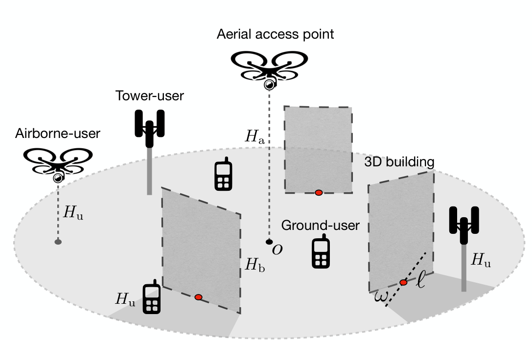
Leveraging UAVs as AAPs has been studied in recent literature [4, 5, 6, 7, 8, 9, 10]. A single-UAV network was proposed in [4], where the network coverage was maximized by optimizing the UAVs’ altitudes. The coverage performance can also be maximized via optimizing the placement of UAVs [5]. In [6], the coverage probability of a finite 3D multi-UAV network was calculated via a stochastic geometric approach. Both network coverage and the sum-rate of a hybrid A2G-D2D network were investigated in [7]. An analytical framework that UAV uses ground-BS for wireless backhaul was proposed in [8] with providing the analysis for success probability of establishing a backhaul link as well as backhaul data rate. In [9], the multiple-input multiple-output (MIMO) non-orthogonal multiple access (NOMA) techniques were used in UAV network and the outage probability and ergodic rate of network were studied based on a stochastic geometry model. In [4, 7, 8], the blockage effects were characterized by a statistical model where the link-level line-of-sight (LOS) probability is approximated as a simple sigmoid function. The parameters of sigmoid function are determined the by buildings’ density, sizes, and heights’ distribution. The model is unsuitable for mmWave A2X networks since it fails to capture the fact that multiple nearby links could be simultaneously blocked by the same building and does not consider the diversity in user types (e.g., their different heights). In [10], a mathematical framework was proposed for studying mmWave A2A networks, in which multiple aerial-users are equipped with antenna arrays. Blocking effects were not included since A2A scenario was assumed to be well above the blockages.
In this paper, we develop an analytical framework for characterizing the blockage effects and connectivity of a mmWave A2X network covered by a single AAP. The 3D buildings are modelled as a Boolean line-segment process with fixed height. Given an arbitrary building, the corresponding blocking area is derived as a function of altitude of AAP, users and buildings’ parameters in’cluding their density, sizes, and heights. Based on the model, the AAP coverage area is maximized (or equivalently the blocking area minimized) by optimizing the altitude of AAP. Furthermore, both upper and lower bounds on the blocking area and a suboptimal result of AAP’s altitude are derived in closed-form. Finally, the spatial average connectivity probability of a typical A2X network is obtained, which may be maximized by optimizing the AAP’s altitude.
II System Model and Performance Metric
Consider a mmWave A2X network as illustrated in Fig. 1. In this letter, we focus on the downlink communication from a typical low-altitude AAP to users with different heights.
II-A Channel Model between AAP and Users
The mmWave channel between the AAP and the different types of users is assumed to be LOS or blocked by a building. For simplicity, we assume the non-LOS (NLOS) signals are completely blocked due to severe propagation loss from penetration and limited reflection, diffraction, or scattering [3]. For the LOS case, the channel is assumed to have path-loss without small-scale fading [11]. We assume perfect 3D beam alignment between AAP and users for maximal directivity gain [10]. For the path-loss model, we assume the reference distance is . The AAP transmission with power and propagation distance is attenuated modelled as where is the path-loss exponent [11]. Let be the thermal noise power normalized by the transmit power . The corresponding signal-to-noise ratio (SNR) received at user is defined as where denotes the beamforming gain. We assume that the user is connected to the AAP if the receive SNR exceeds a given threshold . We say that the AAP has a maximal coverage sphere with the radius . The 2D projection of the coverage sphere of the AAP into the plane with user’s height forms a disk with the radius , called the efficient coverage disk and denoted by . The user is connected to the AAP if its 2D location is inside the efficient coverage disk and the link between the user and the AAP is LOS. For higher users heights, i.e., larger , the efficient coverage disk is larger. Let the center of efficient coverage disk, i.e., the 2D projection of AAP’s location, be the origin denoted by .
II-B 3D Building Model
A 3D building model is adopted to characterize blockage effects where buildings are modelled as the Boolean line-segment process with the same fixed height for tractability [12, 13]. Adding randomness to the buildings height will be left to future work. Specifically, buildings are approximated as line segments with random length on the 2D plane. Although the buildings have polygon shapes in practice, we are interested in their 1D intersections with the communication links and thus assuming their shape as lines is a reasonable approximation. The center locations of the line-segments are modelled as a homogeneous PPP on plane with density . The lengths and orientations of blockage line-segments are independent identically distributed random variables. Let be the distribution of and let be that of . The Boolean line-segments model can be extended to other models as discussed in Remark 2.
II-C Connectivity and Performance Metrics
We assume that all the users can be simultaneously connected to the A2X network if they are in AAP’s coverage sphere and the link between user and AAP is LOS without being blocked by any building. Consider an arbitrary building whose 2D line-segment center is located at . The building results in a blockaging area where the links between users and AAP are fully blocked by the building (see Fig. 2). To measure the network performance, we define the spatial average connectivity probability, denoted by , as the spatial average fraction of the A2X network that is connectable at any time [14]. The is mathematically expressed as
| (1) |
where denotes the size of .
III Analysis For Network Connectivity
III-A Size of Blocking Area
We begin by calculating the size of blocking area for an arbitrary building whose 2D line-segment center located at . We first fix the length and of the typical building. Let be the distance between and . Let be the minimal (shortest) distance between and line-segment (2D projection of building) and be the maximal (longest) distance (see the lines and in Fig. 2). If the AAP’s altitude does not exceed building’s height, i.e., , the size of blocking area (see the gray area covered by in Fig. 2) is calculated by , where and
| (2) |
If , the blocking area could be further reduced since the AAP covers more area via LoS links due to the benefit of higher altitude. Compared with the coverage area of AAP when , we define this additional coverage area due to as the coverage gain, denoted by (see the area covered by (green area) in Fig. 2). Based on the basic geometric calculation, is calculated as
| (3) |
where and . Then, is calculated as follows.
Lemma 1 (Size of ).
The calculations follow from geometry, the detailed proof is omitted due to limited space. To simplify the result in Lemma 1 and obtain more insights therein, both upper and lower bounds of are derived. By assuming the distance between any point on building’s line-segment and has the same value or given in (2), the lower and upper bounds of , denoted by and , are derived as
| (5) |
and is obtained by replacing in with . The result for the bounds of is summarized as follows.
Lemma 2 (Bounds of ).
The bounds for can be treated as the bounds for via substituting (6) into (4): , where and is obtained via replacing in with .
Remark 1 (Optimal Altitude of AAP).
A larger AAP’s altitude can effectively increase the coverage (LoS) area, while shrinking the radius of effective coverage disk. We characterize this behavior by optimizing to obtain a suboptimal solution for . When , we have
| (7) |
Substituting into (4) gives the suboptimal solution of .
Remark 2.
Extending the current building model to any model that each building has a random size in 2D projection, such as rectangle [3] or disk, follows a similar analytical structure. The main difference is that the area of buildings should be included into blocking area . Also, needs to be recalculated based on different building’s shape. For instance, if the 2D projection of a building is modelled as a disk with radius diameter (i.e., cylinder in 3D), the blockaging area is recalculated as , where is lower bounded by .
III-B Network Connectivity Probability
In this section, we calculate the connectivity probability defined in (1). Notice that the spatial correlation between different buildings exsits such as the blocking areas of multiple buildings may overlap with each other. For analytical tractablility, we ignore the spatial correlation of buildings due to overlap in the blockaging area of multiple buildings. This assumption is accurate when density of buildings is not very high, which has been validated in [3]. We derive a lower bound of by jointly using Campbell’s theorem, random shape theory, with the results given in Lemmas 1 and 2.
Theorem 1 (Connectivity Probability of AAP).
Proof: See Appendix -A.
Remark 3.
The lower bound becomes tighter when density of buildings, i.e., , becomes smaller. This is because sparsely deployed buildings result in less spatial correlation.
Remark 4.
Based on the discussion in Remark 1 and expression of , the connectivity probability can also be maximizing by optimizing the APP’s altitude .
IV Simulation Results
In this section, we validate the analytical results via Monte Carlo simulation. The radius of maximal coverage sphere is . The height of building is and that of user is . The density of buildings is . The length and orientation of building’s line-segments follow independently and uniformly distributions. Specifically, is uniformly distributed in and is uniformly distributed in .
Fig. 3 shows the coverage gain calculated via (3) and its bounds , calculated via Lemma 2 versus the altitude of AAP . It is observed that is well bounded by and . The lower bound becomes tighter when is small and the upper bound becomes tighter when is large. This agrees with the intuition because larger or smaller altitude of AAP results in larger or smaller coverage gain, respectively, which makes the bound tighter. Moreover, is maximized via optimizing , which confirms the discussion given in Remark 1.
In Fig. 4, we validate the lower bound of connectivity probability , i.e., , given in Theorem 1 by comparing it with the exact value via Monte Carlo simulation. It is observed that both and decrease with building density . More importantly, becomes tighter when buildings are sparsely deployed, which aligns with the discussion in Remark 3.
V Conclusions and Future Work
In this letter, we propose an analytical framework to define and characterize the connectivity in a mmWave A2X network. Based on the blockage model that buildings are modeled by the Boolean line-segment process with fixed height, we calculate the blockage area due to an arbitrary building and the connectivity probability of an AAP. Moreover, the AAP’s altitude can be optimized to maximize the coverage area as well as the network connectivity. Future work will focus on studying the effects of spatial correlation of buildings on network connectivity and modelling a A2X network including multi-AAP’s connections.
VI Acknowledgments
This work was supported in part by the National Science Foundation under Grant No. ECCS-1711702 and Hong Kong Research Grants Council under the Grants 17209917 and 17259416.
-A Proof of Theorem 1
By omitting the spatial correlations between , connectivity probability defined in (1) is lowered bounded as follows.
| (10) |
where follows the Campbell’s theorem and ramdom shape theory [12]. Based on (4), the blocking area can be upper bounded by . Substituting the result above into (10) gives the lower bound of , say , in Theorem 1.
References
- [1] Y. Zeng, R. Zhang, and T. Lim, “Wireless communications with unmanned aerial vehicles: opportunities and challenges,” IEEE Commun. Mag., vol. 54, pp. 36–42, May 2016.
- [2] Z. Xiao, P. Xia, and X. Xia, “Enabling UAV cellular with millimeter-wave communication: Potentials and approaches,” IEEE Comm. Mag., vol. 54, pp. 66–73, May 2016.
- [3] J. Andrews, T. Bai, M. Kulkarni, A. Alkhateeb, A. Gupta, and R. W. Heath, “Modeling and analyzing millimeter wave cellular systems,” IEEE Trans. Commun., vol. 65, pp. 403–430, Jan. 2017.
- [4] A. Al-Hourani, S. Kandeepan, and S. Lardner, “Optimal LAP altitude for maximum coverage,” IEEE Wireless Comm. Letters, vol. 3, pp. 569–572, Dec. 2014.
- [5] J. Lyu, Y. Zeng, R. Zhang, and T. Lim, “Placement optimization of UAV-mounted mobile base stations,” IEEE Commun. Letters, vol. 21, pp. 604–607, Mar. 2017.
- [6] V. Chetlur and H. Dhillon, “Downlink coverage analysis for a finite 3-D wireless network of unmanned aerial vehicles,” IEEE Trans. Commun., vol. 65, pp. 4543–4558, Oct. 2017.
- [7] M. Mozaffari, W. Saad, M. Bennis, and M. Debbah, “Unmanned aerial vehicle with underlaid device-to-device communications: Performance and tradeoffs,” IEEE Trans. Wireless Commun., vol. 15, pp. 3949–3963, Jun. 2016.
- [8] B. Galkin, J. Kibilda, and L. DaSilva, “A stochastic geometry model of backhaul and user coverage in urban UAV networks,” Available: https://arxiv.org/abs/1710.03701, 2017.
- [9] T. Hou, Y. Liu, Z. Song, X. Sun, and Y. Chen, “Multiple antenna aided NOMA in UAV networks: A stochastic geometry approach,” Available: https://arxiv.org/abs/1805.04985, 2018.
- [10] T. Cuvelier and R. Heath Jr, “Mmwave MU-MIMO for aerial networks,” Available: https://arxiv.org/abs/1804.03295, 2018.
- [11] K. Han, Y. Cui, Y. Wu, and K. Huang, “The connectivity of millimeter wave networks in urban environments modeled using random lattices,” IEEE Trans. Wireless Commun., vol. 17, pp. 3357–3372, May 2018.
- [12] A. Gupta, J. Andrews, and R. Heath Jr, “Macrodiversity in cellular networks with random blockages,” IEEE Trans. Wireless Commun., vol. 17, pp. 996–1010, Feb. 2018.
- [13] X. Li, T. Bai, and R. Heath Jr, “Impact of 3D base station antenna in random heterogeneous cellular networks,” in Proc. of the IEEE WCNC, pp. 2254–2259, Apr. 2014.
- [14] J. Andrews, F. Baccelli, and R. Ganti, “A tractable approach to coverage and rate in cellular networks,” IEEE Trans. Commun., vol. 59, pp. 3122–3134, Nov. 2011.