Dark Matter Particle Explorer observations of high-energy cosmic ray electrons plus positrons and their physical implications
Abstract
The DArk Matter Particle Explorer (DAMPE) is a satellite-borne, high-energy particle and -ray detector, which is dedicated to indirectly detecting particle dark matter and studying high-energy astrophysics. The first results about precise measurement of the cosmic ray electron plus positron spectrum between 25 GeV and 4.6 TeV were published recently. The DAMPE spectrum reveals an interesting spectral softening arount TeV and a tentative peak around TeV. These results have inspired extensive discussion. The detector of DAMPE, the data analysis, and the first results are introduced. In particular, the physical interpretations of the DAMPE data are reviewed.
pacs
95.35.+d,95.85.Ry,96.50.S-,96.50.sbI Introduction
The existence of dark matter (DM) in our Universe is well established by many astronomical and cosmological observations (see reviews [1, 2]). The physical nature of DM, which is largely unknown, becomes one of the most important and fundamental questions of modern physics. The evolution of large scale structures of the Universe and the relic abundance of DM indicates that DM is most probably a kind of weakly interacting massive particle (WIMP) beyond the standard model of particle physics. This postulated weak interaction feature of DM makes it detectable by particle detectors. In general there are three ways proposed to detect WIMP DM: the direct detection of the WIMP-nucleus scattering by underground detectors, the indirect detection of the annihilation/decay of WIMPs, and the production of WIMP pairs in large particle colliders [2, 3]. Quite a number of experiments have been carried out to search for WIMPs since the 1980s [4, 3].
While the direct detection experiments keep on pushing the WIMP-nucleon scattering cross section lower and lower [5, 6, 7], interesting anomalies have been found in cosmic ray (CR) and -ray observations in recent years [8, 9, 10, 11, 12, 13, 14, 15]. Among these anomalies, the biggest puzzle is probably the positron excess discovered11 1 See also earlier hints from HEAT and AMS measurements [16, 17]. by PAMELA [9], Fermi-LAT [11], and AMS-02 [12], and the associated total cosmic ray electron plus positron (CRE) excess by ATIC [8], Fermi-LAT [10], and AMS-02 [13]. The positron and CRE excesses suggest the existence of primary positron and electron sources besides the secondary component from inelastic collisions of CR nuclei and the interstellar medium. No significant excess of CR antiprotons [18, 19, 20] constrains that the primary sources of these CREs should be “leptonic” (see, e.g., [21, 22, 3]). Two leading scenarios to explain the positron and CRE excesses are pulsars [23, 24, 25] and DM annihilation/decay [26, 27, 28]. The DM scenario is severely constrained by the -ray and radio observations [29, 30, 31, 32], leaving pulsars the most likely origin of these excesses. However, the recent observations of TeV -ray emission from two nearby pulsars by HAWC indicated that the CREs from these two pulsars were not enough to account for the positron excess [33], unless a special transportation of CREs was assumed [34, 35]. The origin of the positron and CRE excesses is still not clear yet.
More precise measurements of the spectral behaviors and anisotropies of positrons and/or CREs are particularly helpful in identifying their origin. For example, the fine structures of the CRE spectrum may be used to distinguish pulsar and DM models [36, 37, 38, 39]. The DArk Matter Particle Explorer (DAMPE) is dedicated to precise observations of CREs, -rays, and CR nuclei in space [40, 41]. The major science of DAMPE is to explore the TeV window via CREs and -rays, and to search for possible DM signals. The -ray and nucleus data of DAMPE also enable us to study high-energy astrophysical phenomena and the CR physics [41].
The DAMPE mission was launched into a 500 km Sun-synchronous orbit on December 17, 2015. It has operated smoothly on orbit for more than two years, and has recorded over 4 billion CR events, with a daily event rate of million. All detectors of DAMPE operate perfectly as expected, which brings us new views about the high-energy Universe. The first results about the CRE spectrum based on the first 530 days of data have been published recently [42]. This review introduces the DAMPE mission, the first results, and the proposed physical interpretations (see also Ref. [43] for a mini-review).
II DAMPE experiment
DAMPE is a calorimetric-type, satellite-borne detector. The DAMPE instrument consists of 4 sub-detectors: from top to bottom, the Plastic Scintillator strip Detector (PSD; [44]), the Silicon-Tungsten tracKer-converter (STK; [45]), the BGO imaging calorimeter [46], and the NeUtron Detector (NUD; [47]). The layout of the detector is shown in Fig. 1 [41].

The PSD measures the (absolute) charge of an incident particle via the ionization effect, and serves as an anti-coincidence detector for -rays. The PSD consists of two layers of orthogonally placed plastic scintillator bars, with an effective area of cm2 [41]. In each layer, 41 bars are arranged in two sub-layers with a shift of 0.8 cm to enable a full coverage of incident particles. The overall efficiency of the PSD is about 0.99999 based on Monte Carlo (MC) simulations [48]. The charge resolution of protons, Carbon, and Iron nuclei is found to be about (full width at half maximum), (Gaussian width), and (Gaussian width), respectively [49].
The STK measures the trajectory and the charge of a particle. The STK consists of 6 double-layers of silicon tracker, each layer with two sub-layers arranged orthogonally to measure the and positions of a track. Each silicon layer is made of 16 ladders, each formed by 4 silicon micro-strip detectors (SSD). Each ladder is segmented into 768 strips, half of which are readout strips to limit the number of readout channels. In total there are readout channels of the STK. In addition, three 1 mm thick tungsten plates are inserted to increase the photon conversion rate. The total thickness of the STK is about one radiation length. The spatial resolution of the STK is better than m after the alignment procedure [50]. The angular resolution of the STK based on MC simulations is about () at 1 (100) GeV for normal incident photons [41]. The STK can also measure the particle charge through measuring the ionization energy loss. The charge resolution is found to be about 0.04 for protons and 0.07 for Helium nuclei (both are Gaussian widths; [51]). The STK is helpful in improving the charge resolution of light nuclei. However, it would get saturated when .
The BGO calorimeter is the major detector of DAMPE instrument which measures the energy and trajectory of an incident particle, and most importantly, provides high-performance electron/hadron discrimination based on the shower images. The BGO calorimeter is made of 308 BGO crystals, placed orthogonally in 14 layers. Each crystal is read out at the two ends by photomultiplier tubes coupled to optical filters with different attenuation factors. At each end the signal is read out from three dynodes with different gain. Such a design can enlarge the dynamic range and check the consistency of the energy measurement [46]. The effective area of the calorimeter is cm2, and the thickness is about 32 radiation lengths. This very thick calorimeter enables full development of electro-magnetic showers with primary energies up to 10 TeV without significance leakage [52]. A small fraction of energy leakage () due to dead materials can be corrected with a shower-development-dependent method [52]. The MC simulations show that the energy resolution of electrons and photons can be parameterized as , which is verified by the beam test data from 0.5 GeV to 243 GeV [53]. The energy resolution is about at 1 GeV and above 100 GeV. The absolute energy scale is determined by the geomagnetic cutoff of the CRE spectrum, which gives higher of the energy scale [54]. The linearity of the energy measurement has been well confirmed by the beam test data up to 243 GeV [41]. For protons the energy resolution is about for energies from 10 GeV to 100 TeV [41]. The proton rejection fraction is found to be higher than when keeping of CREs based on a two-parameter representation of shower images [42].
At the bottom is the NUD detector which provides additional electron/hadron discrimination, due to the fact that a hadronic shower typically gives one order of magnitude higher number of neutrons than that of an electromagnetic shower. The NUD is made of four plastic scintillators with (weight) Boron element. The active area of the NUD is about . Neutrons are captured via the reaction , and the ionization energy loss due to charged Lithium and particles can be recorded by photomultiplier tubes. Simulations show that the proton rejection power for NUD can reach a factor of for TeV energies [41].
These four sub-detectors enable good measurements of the charge (), arrival direction, energy, and particle identity of each event. More detailed description of the detector and its simulated performance as well as beam test results can be found in Ref. [41].
III Observations of CREs
The observations of CREs are difficult, since there are large amount of proton and nucleus backgrounds. At GeV energies, the flux of protons is about 100 times higher than that of electrons. The ratio increases with energies, reaching at TeV energies. Any reliable detection of CREs must effectively reject the proton (or more generally, nucleus) background, to a level of or more. Usually the magnetic spectrometer is used for the identification of CREs, such as balloon-borne experiments HEAT, CAPRICE, and space experiments PAMELA, AMS. Another way is to use the imaging calorimeter to distinguish electrons from hadrons, e.g., balloon-borne experiments BETS, ATIC, and space experiments Fermi, DAMPE, CALET. The ground-based imaging atmospheric Cherenkov telescope (IACT) arrays or air shower detector arrays with muon detectors can also distinguish CREs from the hadronic background and measure the CRE spectrum, although there are relatively large systematic uncertainties.


Using 530 days of DAMPE data, the first measurement of the CRE spectrum from 25 GeV to 4.6 TeV was given [42]. We briefly describe the data analysis here. The PSD of DAMPE can effective reject heavy nuclei and -rays, leaving mainly CREs and protons. The shower images in the BGO calorimeter are then used to distinguish CREs from protons [55, 56]. The events with reconstructed tracks passing through the whole detector were selected. An energy-weighted root-mean-square (RMS) value of hit positions in the calorimeter is employed to describe the transverse spread of a shower. The RMS value of the th layer is defined as
| (1) |
where and are coordinate and deposit energy of the th bar in the th layer, and is the coordinate of the shower center of the th layer. The second parameter, , the deposit energy fraction of the last BGO layer, is to describe the tail behavior of a shower. The left panel of Fig. 2 shows the scattering plot of the total RMS values of 14 layers () versus , for events with deposit energies between 500 GeV and 1 TeV. We can clearly see two populations of the data, with the upper one being proton candidates and the lower one being CRE candidates.
To quantify the selection of CREs, these two-dimensional parameter distributions were prejected to one-dimension, with a re-defined parameter . The distributions of for the flight data and MC simulations of electrons and protons are shown in the right panel of Fig. 2. A very good match between the data and simulations can be seen. The CREs are selected with , which results in contamination of the proton background based on a fit with MC templates [42].
In total 1.5 million CREs with energies above 25 GeV are selected in the 2.8 billion events of the data sample. The derived CRE spectrum from 25 GeV to 4.6 TeV [42] is shown in Fig. 3, compared with other measurements. To highlight the high-energy part, we zoom in and show again the spectra above GeV in the right panel of Fig. 3. We can see that the DAMPE data significantly reduces the uncertainties of the measurement for GeV. The direct measurement of the CRE spectrum has been extended to TeV for the first time. Previously, only the IACTs on the ground can reach such high energies, but with quite large systematic uncertainties. The overall behavior of the DAMPE CRE spectrum is consistent with that of Fermi-LAT and HESS. However, for GeV, the DAMPE CRE spectrum is slightly harder than the results of AMS-02 and CALET. The uncertainties of the absolute energy scale of these measurements may partially account for such a disagreement.


The DAMPE spectrum clearly reveals a spectral break at TeV, with the spectral index changing from to . The significance of such a break is estimated to be about . The spectral indices are quite consistent with that of Fermi-LAT below the break and that of IACTs above the break. Previous measurements by IACTs showed only weak evidence for such a spectral break [62]. The Fermi-LAT measurement up to 2 TeV and CALET measurement up to 3 TeV, however, did not show significant spectral break around TeV. This may be due to the relatively high proton background and low energy resolution of Fermi-LAT and low statistics of CALET. There is also an indication of a narrow spectral peak at energies of TeV.
Apart from the spectral break around TeV, the CRE spectra at lower energies are not featureless either. The Voyager spacecraft has travelled for more than 140 astronomical units (AU) away from the earth in about 40 years since 1977, and there was evidence showing that it passed through the heliopause and entered the interstellar space [66]. The CRE spectrum measured by Voyager thus represents the local interstellar (LIS) result without the solar modulation. The other measurements were obtained near the earth, and the low energy parts of the spectra ( GeV) are expected to be suppressed by the solar magnetic field. There is a break of the CRE spectrum around a few GeV, with spectral indices changing from about 22 2 This value depends on solar activities during the measurement. to [13]. The Fermi-LAT data reveals a second break (hardening) at GeV, and the spectral index changes from to [60]. We leave the interpretation of the CRE spectral behaviors in Sec. IV.
IV Physical implications
IV.1 CRE propagation in the Milky Way
Before discussing the physical modeling of the CRE spectrum, we briefly introduce the propagation of CREs. The propagation of CREs in the Milky Way can be described by a diffusion-cooling eauqtion
| (2) |
where is the diffusion coefficient, is the cooling rate, and is the source injection term. This equation is valid at high energies (e.g., GeV) where cooling is important. At low energies other physical processes such as reacceleration or convection may be important [67].
Assuming a spherically symmetric geometry with infinite boundary conditions, the Green’s function of Eq. (2) with respect to and (for -type source function in space and time) is [68]
| (3) |
Here with the injection energy spectrum of electrons, is the initial energy of an electron which is cooled down to within time , and
| (4) |
is the effective propagation distance of an electron before getting cooled. The convolution of Eq. (3) with the source spatial distribution and injection history gives the propagated electron fluxes at the Earth’s location. Fig. 4 gives the cooling time () and effective propagation distance (right) of CREs, for typical diffusion and cooling parameters (see Ref. [69]). We find that, for TeV electrons, the cooling time is only about Myr and the propagation distance is about kpc, which means that TeV electrons can only come from nearby and fresh sources.

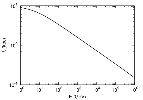
Fig. 5 illustrates the relative (logarithmic) probability of observing an electron with specified energy from a source located at different distance from the Earth (image center), assuming a continuous injection of an power-law. The plane refers to the Galactic plane, and the direction points to the Galactic poles. This plot shows again that high energy CREs should have a local origin.


IV.2 Overall modeling of the CRE spectrum and the positron excess
The CREs defined in this review include both electrons and positrons. It has been widely accepted that these CREs consist of several components:
- •
Primary electrons which are accelerated in accompany with nuclei CRs by Galactic acceleration sources, e.g., supernova remnants.
- •
Secondary electrons and positrons from the inelastic collisions between CR nuclei (mostly protons and Helium nuclei) and the interstellar medium (ISM).
- •
For energies from 0.5 GeV to GeV, the positron fraction in CREs is about [70]. Thus the CRE flux is dominated by primary electrons in such an energy range. At higher energies, the behavior of the positron fraction is not clear yet, and whether the primary electrons can still dominate or not is not sure.
The overall CRE spectrum and positron fraction can be understood in such a three-component scenario. The first spectral break at several GeV is due to several effects. The ionization and Coulomb cooling plays a significant role in regulating the low-energy (GeV) spectrum of CREs [71]. The fit to the data further suggests a break of the injection spectrum at a few GeV [72, 73]. The observations of -ray emission from supernova remnants did suggest a broken power-law form of the particle spectrum [74]. The underlying physics of such an injection break is not clear yet. It was proposed that strong ion-neutral collisions near the shock fronts of CR acceleration sources [75] or the escape of particles from/into finite-size region might lead to this break [76, 77]. The solar modulation suppresses the low-energy flux more than the high-energy flux, and also contribute to form a break. All these effects together give the observed spectral break at a few GeV.
Quantitative fitting to the positron fraction and CRE spectra with those three components, assuming either pulsars or DM annihilation/decay as the source(s) of the additional electrons and positrons, shows that a spectral hardening around GeV of the primary electron component is required [78, 79, 80] (see also [81, 82]). Fig. 6 shows the comparison of the fitting results for the model without (top two panels) and with (bottom two panels) the spectral hardening of the primary electrons. The fit can be improved significantly when including the spectral hardening. The origin of the spectral hardening, as well as the TeV break revealed by HESS/DAMPE (discussed in more details below), may be due to the breakdown of continuous source distribution and imprints of nearby source(s) [83, 84, 85].


IV.3 Implication of the TeV spectral break
The spectral break around TeV as observed by IACTs and DAMPE has very interesting physical implications. The precise CRE spectrum by DAMPE can significantly narrow down the parameter space of models, either astrophysical ones or DM annihilation/decay, to explain the positron excess [69]. Fig. 7 shows the constraints on some parameters of the pulsar model (left) and the DM annihilation model (right). To give such constraints, we again assume the three-component model as described above, and add an exponential cutoff with characteristic energy of the primary electron spectrum. The injection spectrum of electrons and positrons from pulsars is parameterized as an exponential cutoff power-law form, with cutoff energy . For the DM annihilation model, the density profile is assumed to be a Navarro-Frenk-White form [86], and the annihilation channel is . Two results are compared: the fitting to pre-DAMPE CRE data (i.e., AMS-02 and HESS) and to the DAMPE data. In both fittings the AMS-02 positron fraction is included. It shows that the DAMPE data reduce the parameter space remarkably. Most importantly, improved constraints on the model parameters lead to robust exclusion of the simple DM annihilation or decay models to account for the positron excess, when considering the constraints from the cosmic microwave background (CMB; [87]) and Fermi-LAT -ray observations [88, 89], as shown in Fig. 8. Note that in Ref. [69] the fittings for the channel of the DM models are poor with too large values. Therefore the corresponding contours in Fig. 8 for such a channel are statistically less meaningful. For other channels the fittings are acceptable.


The TeV break could be naturally explained by one or a few nearby source(s). The cooling effect during the propagation of CREs could form a cutoff of the detected spectrum (e.g., [68, 83]). This “knee-like” structure might also be due to the maximum energy of CREs injected into the Milky Way. In Ref. [90] it was proposed that the confinement and radiative cooling of electrons during the acceleration in supernova remnants could account for this CRE knee. Such electrons escape from the sources after yr when the supernova remnants merge into the ISM, and the resulting CRE spectrum naturally cuts off around TeV [91]. This scenario may work. We just emphasize the importance of discretness of the source distribution for understanding the TeV spectrum of CREs. Assuming a supernova rate of per year, the estimated number of supernovae within the cooling time and the effective propagation distance is for TeV electrons. Therefore the active sources of TeV CREs should be discrete.
IV.4 Discussion on the tentative 1.4 TeV structure
The tentative peak structure at TeV, if gets confirmed with more data, is completely unexpected. We emphasize that the current data is not significant enough to draw a conclusion. The local significance is estimated to be about assuming a broken power-law background [92, 93]. If the look-elsewhere effect is taken into account, the estimated global significance is about [93]. Note, however, the significance estimate depends on the background adopted, as illustrated in Ref. [94]. Nevertheless, given the potential importance of such a structure, quite a number of works appeared to discuss its possible implications [69, 92, 95, 121, 122, 96, 97, 98, 99, 100, 101, 123, 102, 124, 103, 125, 104, 105, 106, 107, 126, 108, 109, 110, 111, 127, 112, 113, 114, 115, 128, 94, 116, 117, 118, 119, 120].
We summarize some general requirements to account for the data. First is about the energetics. We discuss two kinds of injection modes of the sources: instantaneous injection and continuous injection. For instantaneous injection, the total energy of the source is required to be [69]
| (5) | |||||
where is the age of the source and is the energy density of the peak. This total energy release ( erg depending on different injection time) is a little bit smaller but still comparable to a typical pulsar [39]. For continuous injection, the source luminosity is [69]
| (6) | |||||
where is the source distance. If the DM annihilation is assumed to be continuous source of those CREs, the average density of DM is about TeV cm-3 for a region of kpc, TeV, and a thermal annihilation cross section, which is about 30 times higher than the canonical local density. This means a local DM subhalo or a density enhancement is required [69, 92, 109]. To account for the data, the subhalo mass is found to be about M⊙ or the local density is enhanced by a factor of . Such a requirement is extreme according to numerical simulations of DM structures, and thus some other mechanisms are necessary to boost the cross section or density distribution, e.g., a mini-spike or an ultra-compact micro halo [92, 114].
As described above, the strong cooling of CREs limited the propagation distance of an electron before losing most of its energy. For TeV electrons, such a distance is about 1 kpc [69]. The spectral shape gives further constraints on the source distance. If the distance is too large, the cooling effect would broaden the CRE spectrum, making it difficult to fit the data. Typically the distance is required to be smaller than kpc [69, 92]. Fig. 9 illustrates the constraints on the distance and injection energy of a continuous point-like source with a Gaussian injection spectrum [92]. In Ref. [92] it was suggested that for the instantaneous injection scenario, a source with a distance of kpc could also give a sharp spectrum. This is due to that low-energy particles are not able to propagate to such a distance, while high-energy electrons have already cooled down. A caution is that this scenario may need a quite large energy output into electrons/positrons from the source, erg.

The injection spectrum can also not be arbitrary. In general the propagation will make the CRE spectrum broader than the injection one. Therefore to give a narrow peak around the Earth, the injection spectrum should also be quasi-monochromatic. For the DM annihilation/decay, the direct channel is required. Astrophysically it is not easy to generate quasi-monochromatic spectra. We found a possible exception is the cold, ultra-relativistic plasma wind from pulsars [129, 130, 131]. The Lorentz factor of the bulk flow of pulsar winds is suggested to be , which just corresponds to the energy of the DAMPE peak. However, there should not be significant energy loss or gain of such pulsar wind during their transportation outwards through the pulsar wind nebula. Otherwise the narrow injection spectrum cannot be maintained. A good fit to the data with reasonable pulsar model parameters was given in Ref. [69]. The model details, as well as the escape from the nebula, need further studies. The injection spectrum can be softer for a larger distance of the source [92]. However, it is still quite hard () compared with canonical prediction of shock acceleration.
Within the DM annihilation/decay scenario from a local clump, many works investigate the potential particle model extension of the standard model. A general requirement is that DM particles should couple with electrons (leptons) instead of quarks. A simple extension is to add a symmetry to the standard model, and the DM annihilate into electrons (leptons) via the new gauge boson mediator, e.g., a [95, 121, 122, 96, 97, 98, 99, 100, 101, 123, 102, 124, 103]. In the fermion DM case, the Dirac type is more natural as its cross section is -wave dominant for the -channel annihilation process . Also several bosonic DM models were developed with different Higgs potentials and Yukawa terms. Some of such models are realized in different kinds of seesaw models [95, 125, 104, 105, 124, 99]. Other attempts include the lepton portal DM model in which DM particles interact with standard model particles through mediators with lepton numbers [69, 107], or the lepton-flavored DM model in which DM particles carry lepton numbers themselves [108]. The singlet scalar DM model [111], higgs triplet with vector DM model [127], graviton-mediated DM model [113], Quasi-degenerate DM model [112], lepton-specific interaction DM model [128], and left-right symmetric scalar DM model [117] were also presented.
Contraints on the DM models with direct detection and collider data have been discussed in some models (e.g., [95, 122, 121, 107, 96, 126]). Since in general the DM directly or indirectly couples with leptons in these models, the DM-nucleon scattering is induced through the lepton-loop and photon mediator. The constraints from the current direct detection data are relatively weak. It was shown that for some particular types of interactions, the direct detection data can exclude a considerable part of the parameter space [122, 108, 100, 101]. Such interaction can also contribute to the lepton-nucleon scattering through the Drell-Yan process, which is also significantly lower than the current LHC sensitivity [122]. The constraints from null detection of the leptophilic bosons [126, 100, 101, 102, 103, 124] and the anomalous magnetic moments of leptons [122, 126, 101, 103] were also discussed. It needs to be noted that if there is indeed a massive subhalo in the local vicinity of the solar system, the local density of DM should be different from the canonical one of GeV cm-3 [132]. For example, for a distance of 0.1 kpc and a subhalo mass of () M⊙, the local density becomes (19) times as large as the canonical value. Therefore, any direct detection limits based on the canonical local density should be lower by such a factor. While the model predictions may still be consistent with the current data, the future direct detection and collider experiments can definitely probe a large portion of the model parameters, as illustrated in Ref. [95].
Other than the DM annihilation/decay, some models with additional exotic physical processes have also been proposed. In Ref. [119] a threshold interaction with a hypothetical light particle was employed to explain the knee and also the peak of the DAMPE data. In Ref. [120] a gluon condensation effect during the hadronic interaction of nuclei was proposed. The future observations of multi-messengers, including -rays, neutrinos, anisotropy of CREs, may help test both the DM models and these exotic physical models (see e.g., [95, 116]).
V Summary
Recently the DAMPE collaboration reported the measurement of the high-energy CRE spectrum with very high precision. Here the DAMPE experiment, data analysis, and the physical interpretations of its results are reviewed. The DAMPE CRE data, which is by far the most precise in the TeV band, improves significantly the constraints on the model parameters to explain CREs. Remarkably, the DM annihilation/decay models to explain the positron excess and CRE spectra can be largely excluded with joint efforts of AMS-02, DAMPE, Fermi, and PLANCK. One may either need to finely tune the DM models with more complicated assumptions or resort to astrophysical solutions to the positron anomaly. A tentative peak structure around TeV can be seen in the CRE spectrum. If it is confirmed by more data, this would be a very interesting and important discovery which is unexpected before. To produce such a spectral feature, the sources of CREs are in general required to be 1) nearby (with a distance kpc) and 2) spectrally hard (or even quasi-monochromatic). The cold, ultra-relativistic wind from pulsars without modification of energies of such wind particles, or the DM annihilation/decay in a nearby subhalo are suggested to account for the data. We emphasize again that the most important things to crucially address this issue are to accumulate more data with DAMPE, and to improve the analysis method to reduce the systematic uncertainties.
Acknowledgements
We thank Dr. Yi-Zhong Fan for helpful discussion. This work is supported by the National Key Research and Development Program of China (No. 2016YFA0400200), National Natural Science Foundation of China (Nos. 11722328, 11773075, U1738205), the 100 Talents Program of Chinese Academy of Sciences, and the Youth Innovation Promotion Association of Chinese Academy of Sciences (No. 2016288).
References
- [1] G. Jungman, M. Kamionkowski, and K. Griest, Phys. Rept. 267, 195 (1996).
- [2] G. Bertone, D. Hooper, and J. Silk, Phys. Rept. 405, 279 (2005).
- [3] X.-J. Bi, P.-F. Yin, and Q. Yuan, Front. Phys. 8, 794 (2013).
- [4] P. F. Smith and J. D. Lewin, Phys. Rept. 187, 203 (1990).
- [5] D. S. Akerib, et al. (LUX collaboration), Phys. Rev. Lett. 118, 021303 (2017).
- [6] E. Aprile, et al. (XENON collaboration), Phys. Rev. Lett. 119, 181301 (2017).
- [7] X. Cui, et al. (PandaX collaboration), Phys. Rev. Lett. 119, 181302 (2017).
- [8] J. Chang, et al. (ATIC collaboration), Nature 456, 362 (2008).
- [9] O. Adriani, et al. (PAMELA collaboration), Nature 458, 607 (2009).
- [10] A. A. Abdo, et al. (Fermi collaboration), Phys. Rev. Lett. 102, 181101 (2009).
- [11] M. Ackermann, et al. (Fermi collaboration), Phys. Rev. Lett. 108, 011103 (2012).
- [12] M. Aguilar, et al. (AMS collaboration), Phys. Rev. Lett. 110, 141102 (2013).
- [13] M. Aguilar, et al. (AMS collaboration), Phys. Rev. Lett. 113, 221102 (2014).
- [14] D. Hooper and L. Goodenough, Phys. Lett. B 697, 412 (2011).
- [15] M. Ackermann, et al. (Fermi collaboration), Astrophys. J. 840, 43 (2017).
- [16] S. W. Barwick, et al. (HEAT collaboration), Astrophys. J. Lett. 482, L191 (1997).
- [17] M. Aguilar, et al. (AMS collaboration), Phys. Lett. B 646, 145 (2007).
- [18] O. Adriani, et al. (PAMELA collaboration), Phys. Rev. Lett. 102, 051101 (2009).
- [19] O. Adriani, et al. (PAMELA collaboration), Phys. Rev. Lett. 105, 121101 (2010).
- [20] M. Aguilar, et al. (AMS collaboration), Phys. Rev. Lett. 117, 091103 (2016).
- [21] Y.-Z. Fan, B. Zhang, and J. Chang, Int. J. Mod. Phys. D 19, 2011 (2010).
- [22] P. D. Serpico, Astropart. Phys. 39, 2 (2012).
- [23] C. S. Shen, Astrophys. J. Lett. 162, L181 (1970).
- [24] D. Hooper, P. Blasi, and P. Dario Serpico, J. Cosmol. Astropart. Phys. 1, 25 (2009).
- [25] H. Yuksel, M. D. Kistler, and T. Stanev, Phys. Rev. Lett. 103, 051101 (2009).
- [26] L. Bergstrom, T. Bringmann, and J. Edsjo, Phys. Rev. D 78, 103520 (2008).
- [27] M. Cirelli, M. Kadastik, M. Raidal, and A. Strumia, Nucl. Phys. B 813, 1 (2009).
- [28] P. F. Yin, Q. Yuan, J. Liu, J. Zhang, X. J. Bi, S. H. Zhu, and X. M. Zhang, Phys. Rev. D 79, 023512 (2009).
- [29] G. Bertone, M. Cirelli, A. Strumia, and M. Taoso, J. Cosmol. Astropart. Phys. 3, 9 (2009).
- [30] L. Bergstrom, G. Bertone, T. Bringmann, J. Edsjo, and M. Taoso, Phys. Rev. D 79, 081303 (2009).
- [31] M. Papucci and A. Strumia, J. Cosmol. Astropart. Phys. 3, 14 (2010).
- [32] M. Cirelli, P. Panci, and P. D. Serpico, Nucl. Phys. B 840, 284 (2010).
- [33] A. U. Abeysekara, et al. (HAWC collaboration), Science 358, 911 (2017).
- [34] D. Hooper, I. Cholis, T. Linden, and K. Fang, Phys. Rev. D 96, 103013 (2017).
- [35] K. Fang, X.-J. Bi, P.-F. Yin and Q. Yuan, ArXiv e-prints (2018), 1803.02640.
- [36] J. Hall and D. Hooper, Phys. Lett. B 681, 220 (2009).
- [37] D. Malyshev, I. Cholis, and J. Gelfand, Phys. Rev. D 80, 063005 (2009).
- [38] M. Pato, M. Lattanzi, and G. Bertone, J. Cosmol. Astropart. Phys. 12, 20 (2010).
- [39] P.-F. Yin, Z.-H. Yu, Q. Yuan, and X.-J. Bi, Phys. Rev. D 88, 023001 (2013).
- [40] J. Chang, Chin. J. Space Sci. 34, 550 (2014).
- [41] J. Chang, et al. (DAMPE Collaboration), Astropart. Phys. 95, 6 (2017).
- [42] G. Ambrosi, et al. (DAMPE Collaboration), Nature 552, 63 (2017).
- [43] Y. Genolini, ArXiv e-prints (2018), 1806.06534.
- [44] Y. Yu, et al., Astropart. Phys. 94, 1 (2017).
- [45] P. Azzarello, et al., Nucl. Instrum. Meth. A 831, 378 (2016).
- [46] Z. Zhang, Y. Zhang, J. Dong, S. Wen, C. Feng, C. Wang, Y. Wei, X. Wang, Z. Xu, and S. Liu, Nucl. Instrum. Meth. A 780, 21 (2015).
- [47] M. He, T. Ma, J. Chang, Y. Zhang, Y. Y. Huang, J. J. Zang, J. Wu, and T. K. Dong, Acta Astronomica Sinica 57, 1 (2016).
- [48] Z.-L. Xu, et al., Res. Astron. Astrophys. 18, 027 (2018).
- [49] T.-K. Dong, et al., Res. Astron. Astrophys. to be submitted (2018).
- [50] A. Tykhonov, et al., Nucl. Instrum. Meth. A 893, 43 (2018).
- [51] S. Vitillo and V. Gallo, Proc. Sci. ICRC2017, 240 (2017).
- [52] C. Yue, J. Zang, T. Dong, X. Li, Z. Zhang, S. Zimmer, W. Jiang, Y. Zhang, and D. Wei, Nucl. Instrum. Meth. A 856, 11 (2017).
- [53] Z. Zhang, et al., Nucl. Instrum. Meth. A 836, 98 (2016).
- [54] J.-J. Zang, C. Yue, and X. Li, Proc. Sci. ICRC2017, 197 (2017).
- [55] J. Chang, Int. Cosmic Ray Conf. 5, 37 (1999).
- [56] J. Chang, et al., Adv. Space Res. 42, 431 (2008).
- [57] A. C. Cummings, E. C. Stone, B. C. Heikkila, N. Lal, W. R. Webber, G. Johannesson, I. V. Moskalenko, E. Orlando, and T. A. Porter, Astrophys. J. 831, 18 (2016).
- [58] M. A. DuVernois, et al., Astrophys. J. 559, 296 (2001).
- [59] S. Torii, et al., Astrophys. J. 559, 973 (2001).
- [60] S. Abdollahi, et al. (Fermi Collaboration), Phys. Rev. D 95, 082007 (2017).
- [61] O. Adriani, et al. (CALET Collaboration), Phys. Rev. Lett. 119, 181101 (2017).
- [62] F. Aharonian, et al. (H.E.S.S. Collaboration), Phys. Rev. Lett. 101, 261104 (2008).
- [63] F. Aharonian, et al. (H.E.S.S. Collaboration), Astron. Astrophys. 508, 561 (2009).
- [64] D. Borla Tridon, et al. (MAGIC collaboration), Int. Cosmic Ray Conf. 6, 47 (2011).
- [65] D. Staszak, et al. (VERITAS Collaboration), Int. Cosmic Ray Conf. 34, 411 (2015).
- [66] E. C. Stone, A. C. Cummings, F. B. McDonald, B. C. Heikkila, N. Lal, and W. R. Webber, Science 341, 150 (2013).
- [67] T. Delahaye, R. Lineros, F. Donato, N. Fornengo, J. Lavalle, P. Salati, and R. Taillet, Astron. Astrophys. 501, 821 (2009).
- [68] A. M. Atoyan, F. A. Aharonian, and H. J. Volk, Phys. Rev. D 52, 3265 (1995).
- [69] Q. Yuan, et al., ArXiv e-prints (2017), 1711.10989.
- [70] L. Accardo, et al. (AMS Collaboration), Phys. Rev. Lett. 113, 121101 (2014).
- [71] I. V. Moskalenko and A. W. Strong, Astrophys. J. 493, 694 (1998).
- [72] J. Liu, Q. Yuan, X.-J. Bi, H. Li, and X. Zhang, Phys. Rev. D 85, 043507 (2012).
- [73] Q. Yuan, X.-J. Bi, G.-M. Chen, Y.-Q. Guo, S.-J. Lin, and X. Zhang, Astropart. Phys. 60, 1 (2015).
- [74] M. Ackermann, et al. (Fermi Collaboration), Science 339, 807 (2013).
- [75] M. A. Malkov, P. H. Diamond, and R. Z. Sagdeev, Nature Commun. 2, 194 (2011).
- [76] Y. Ohira, K. Murase, and R. Yamazaki, Mon. Not. Roy. Astron. Soc. 410, 1577 (2011).
- [77] H. Li and Y. Chen, Mon. Not. Roy. Astron. Soc. 409, L35 (2010).
- [78] Q. Yuan and X.-J. Bi, Phys. Lett. B 727, 1 (2013).
- [79] Q. Yuan and X.-J. Bi, J. Cosmol. Astropart. Phys. 3, 033 (2015).
- [80] S.-J. Lin, Q. Yuan, and X.-J. Bi, Phys. Rev. D 91, 063508 (2015).
- [81] L. Feng, R.-Z. Yang, H.-N. He, T.-K. Dong, Y.-Z. Fan, and J. Chang, Phys. Lett. B 728, 250 (2014).
- [82] I. Cholis and D. Hooper, Phys. Rev. D 88, 023013 (2013).
- [83] F. A. Aharonian, A. M. Atoyan, and H. J. Voelk, Astron. Astrophys. 294, L41 (1995).
- [84] M. Di Mauro, F. Donato, N. Fornengo, R. Lineros, and A. Vittino, J. Cosmol. Astropart. Phys. 4, 006 (2014).
- [85] K. Fang, B.-B. Wang, X.-J. Bi, S.-J. Lin, and P.-F. Yin, Astrophys. J. 836, 172 (2017).
- [86] J. F. Navarro, C. S. Frenk, and S. D. M. White, Astrophys. J. 490, 493 (1997).
- [87] P. A. R. Ade, et al. (Planck Collaboration), Astron. Astrophys. 594, A13 (2016).
- [88] X. Huang, Y.-L. S. Tsai, and Q. Yuan, Comput. Phys. Commun. 213, 252 (2017).
- [89] M. Ackermann, et al. (Fermi Collaboration), Astrophys. J. 799, 86 (2015).
- [90] K. Fang, X.-J. Bi, and P.-F. Yin, Astrophys. J. 854, 57 (2018).
- [91] V. N. Zirakashvili and F. Aharonian, Astron. Astrophys. 465, 695 (2007).
- [92] X.-J. Huang, Y.-L. Wu, W.-H. Zhang, and Y.-F. Zhou, ArXiv e-prints (2017), 1712.00005.
- [93] A. Fowlie, Phys. Lett. B 780, 181 (2018).
- [94] S.-F. Ge, H.-J. He, and Y.-C. Wang, Phys. Lett. B 781, 88 (2018).
- [95] Y.-Z. Fan, W.-C. Huang, M. Spinrath, Y.-L. Sming Tsai, and Q. Yuan, Phys. Lett. B 781, 83 (2018).
- [96] W. Chao and Q. Yuan, ArXiv e-prints (2017), 1711.11182.
- [97] J. Cao, L. Feng, X. Guo, L. Shang, F. Wang, and P. Wu, ArXiv e-prints (2017), 1711.11452.
- [98] X. Liu and Z. Liu, ArXiv e-prints (2017), 1711.11579.
- [99] P.-H. Gu, ArXiv e-prints (2017), 1711.11333.
- [100] G. H. Duan, X.-G. He, L. Wu, and J. M. Yang, ArXiv e-prints (2017), 1711.11563.
- [101] K. Ghorbani and P. H. Ghorbani, ArXiv e-prints (2017), 1712.01239.
- [102] N. Okada and O. Seto, ArXiv e-prints (2017), 1712.03652.
- [103] T. Nomura, H. Okada, and P. Wu, ArXiv e-prints (2018), 1801.04729.
- [104] T. Nomura and H. Okada, ArXiv e-prints (2017), 1712.00941.
- [105] Y. Sui and Y. Zhang, ArXiv e-prints (2017), 1712.03642.
- [106] L. Zu, C. Zhang, L. Feng, Q. Yuan, and Y.-Z. Fan, ArXiv e-prints (2017), 1711.11052.
- [107] Y.-L. Tang, L. Wu, M. Zhang, and R. Zheng, ArXiv e-prints (2017), 1711.11058.
- [108] W. Chao, H.-K. Guo, H.-L. Li, and J. Shu, ArXiv e-prints (2017), 1712.00037.
- [109] H.-B. Jin, B. Yue, X. Zhang, and X. Chen, ArXiv e-prints (2017), 1712.00362.
- [110] Y. Gao and Y.-Z. Ma, ArXiv e-prints (2017), 1712.00370.
- [111] J.-S. Niu, T. Li, R. Ding, B. Zhu, H.-F. Xue, and Y. Wang, ArXiv e-prints (2017), 1712.00372.
- [112] P.-H. Gu, ArXiv e-prints (2017), 1712.00922.
- [113] R. Zhu and Y. Zhang, ArXiv e-prints (2017), 1712.01143.
- [114] F. Yang, M. Su, and Y. Zhao, ArXiv e-prints (2017), 1712.01724.
- [115] R. Ding, Z.-L. Han, L. Feng, and B. Zhu, ArXiv e-prints (2017), 1712.02021.
- [116] Y. Zhao, K. Fang, M. Su, and M. C. Miller, ArXiv e-prints (2017), 1712.03210.
- [117] J. Cao, X. Guo, L. Shang, F. Wang, P. Wu, and L. Zu, ArXiv e-prints (2017), 1712.05351.
- [118] J.-S. Niu, T. Li, and F.-Z. Xu, ArXiv e-prints (2017), 1712.09586.
- [119] C. Jin, W. Liu, H.-B. Hu, and Y.-Q. Guo, ArXiv e-prints (2016), 1611.08384.
- [120] W. Zhu, J. Lan, J. Ruan, and F. Wang, ArXiv e-prints (2017), 1712.07868.
- [121] P.-H. Gu and X.-G. He, Phys. Lett. B 778, 292 (2018).
- [122] G. H. Duan, L. Feng, F. Wang, L. Wu, J. M. Yang, and R. Zheng, J. High Energy Phys. 2, 107 (2018).
- [123] J. Cao, L. Feng, X. Guo, L. Shang, F. Wang, P. Wu, and L. Zu, Eur. Phys. J. C 78, 198 (2018).
- [124] Z.-L. Han, W. Wang, and R. Ding, Eur. Phys. J. C 78, 216 (2018).
- [125] T. Li, N. Okada, and Q. Shafi, Phys. Lett. B 779, 130 (2018).
- [126] P. Athron, C. Balazs, A. Fowlie, and Y. Zhang, J. High Energy Phys. 2, 121 (2018).
- [127] C.-H. Chen, C.-W. Chiang, and T. Nomura, Phys. Rev. D 97, 061302 (2018).
- [128] G. Liu, F. Wang, W. Wang, and J.-M. Yang, Chin. Phys. C 42, 035101 (2018).
- [129] C. F. Kennel and F. V. Coroniti, Astrophys. J. 283, 694 (1984).
- [130] F. A. Aharonian, S. V. Bogovalov, and D. Khangulyan, Nature 482, 507 (2012).
- [131] F. Aharonian, D. Khangulyan, and D. Malyshev, Astron. Astrophys. 547, A114 (2012).
- [132] Y. Huang, et al., Mon. Not. Roy. Astron. Soc. 463, 2623 (2016).