Efficient Gauss-Newton-Krylov momentum conservation constrained PDE-LDDMM using the band-limited vector field parameterization

Monica Hernandez Affiliation: Computer Sciences Department
Aragon Institute on Engineering Research
University of Zaragoza
mhg@unizar.es

Abstract

The class of non-rigid registration methods proposed in the framework of PDE-constrained Large Deformation Diffeomorphic Metric Mapping is a particularly interesting family of physically meaningful diffeomorphic registration methods. PDE-constrained LDDMM methods are formulated as constrained variational problems, where the different physical models are imposed using the associated partial differential equations as hard constraints. Inexact Newton-Krylov optimization has shown an excellent numerical accuracy and an extraordinarily fast convergence rate in this framework. However, the Galerkin representation of the non-stationary velocity fields does not provide proper geodesic paths. In a previous work, we proposed a method for PDE-constrained LDDMM parameterized in the space of initial velocity fields under the EPDiff equation. The proposed method provided geodesics in the framework of PDE-constrained LDDMM, and it showed performance competitive to benchmark PDE-constrained LDDMM and EPDiff-LDDMM methods. However, the major drawback of this method was the large memory load inherent to PDE-constrained LDDMM methods and the increased computational time with respect to the benchmark methods. In this work we optimize the computational complexity of the method using the band-limited vector field parameterization closing the loop with our previous works.

Keywords:

PDE-constrained, diffeomorphic registration, Gauss-Newton-Krylov optimization, geodesic shooting, incremental adjoint Jacobi equations, band-limited vector field

1 Introduction

Deformable image registration is the process of computing spatial transformations between different images so that corresponding points represent the same anatomical location. There exists a vast literature on deformable image registration methods with differences on the transformation characterization, regularizers, image similarity metrics, optimization methods, and additional constraints [1]. In the last two decades, diffeomorphic registration has arisen as a powerful paradigm for deformable image registration [2]. Diffeomorphisms (i.e., smooth and invertible transformations) have become fundamental inputs in Computational Anatomy. There exist different big families of diffeomorphic registration methods. Our attention in the last years has been focused to PDE-constrained diffeomorphic registration due to its relevance in the last decade.

PDE-constrained diffeomorphic registration augments the original variational formulation with Partial Differential Equations (PDEs) of interest. The framework seems to be very appropriate for the computation of physically meaningful transformations. The first method was proposed by Hart et al. [3]. In that work, the problem was formulated as a PDE-constrained control problem subject to the state PDE and the relationship with Beg et al. LDDMM [4] was stated. Later on, Vialard et al. proposed a PDE-constrained method parameterized on the initial momentum [5]. More recently, Mang et al. have proposed a PDE-constrained method that extended the gradient-descent optimization in Hart et al. approach to inexact Newton-Krylov optimization [6]. In a previous ArXiv publication, we have bridged the gap between Vialard et al. and Mang et al. work by proposing a novel PDE-constrained LDDMM method parameterized on the initial momentum [7]. In addition we have faced the huge computational complexity of PDE-constrained LDDMM using the band-limited vector field parameterization [8, 9].

This work closes the loop between our previous works [8, 9, 7] by formulating the method in [7] in the space of band-limited vector fields. This document is intended to be a self contained equation guide of all the related methods and provide the equations of the closing loop methods. The results section shows, as a proof of concept, the potential of our efficient method for Computational Anatomy applications.

2 Related Methods

2.1 LDDMM

Let $I_{0}$ , and $I_{1}$ be the source and the target images defined on the image domain $\Omega\subseteq\mathbb{R}^{d}$ . We denote with $Diff(\Omega)$ to the Riemannian manifold of diffeomorphisms on $\Omega$ . $V$ is the tangent space of the Riemannian structure at the identity diffeomorphism, $id$ . $V$ is made of smooth vector fields on $\Omega$ . The Riemannian metric is defined from the scalar product in $V$

\langle v,w\rangle_{V}=\langle Lv,w\rangle_{L^{2}}=\int_{\Omega}\langle Lv(x),w(x)\rangle d\Omega,

(1)

where $L=(Id-\alpha\Delta)^{s},\alpha>0,s\in\mathbb{N}$ is the invertible self-adjoint differential operator associated with the differential structure of $Diff(\Omega)$ . We denote with $K$ to the inverse of $L$ .

The LDDMM variational problem is given by the minimization of the energy functional

E(v)=\frac{1}{2}\int_{0}^{1}\langle Lv_{t},v_{t}\rangle_{L^{2}}dt+\frac{1}{\sigma^{2}}\|I_{0}\circ(\phi^{v}_{1})^{-1}-I_{1}\|_{L^{2}}^{2}.

(2)

The problem is posed in the space of time-varying smooth flows of velocity fields in $V$ , ${v}\in L^{2}([0,1],V)$ . Given the smooth flow ${v}:[0,1]\rightarrow V$ , $v_{t}:\Omega\rightarrow\mathbb{R}^{d}\in V$ , the diffeomorphism $\phi_{1}^{v}$ is defined as the solution at time $1$ to the transport equation $d_{t}\phi_{t}^{v}=v_{t}\circ\phi_{t}^{v}$ with initial condition $\phi_{0}^{v}=id$ . The transformation $(\phi^{v}_{1})^{-1}$ computed from the minimum of $E({v})$ is the diffeomorphism that solves the LDDMM registration problem between $I_{0}$ and $I_{1}$ . The optimization of Equation 2 was originally approached in [4] using gradient-descent in $L^{2}([0,1],V)$ , yielding the update equation

v_{t}^{n+1}=v_{t}^{n}-\epsilon(\nabla_{v}E(v))_{t}.

(3)

2.2 EPDiff-LDDMM

The geodesics of $Diff(\Omega)$ under the right-invariant Riemannian metric are uniquely determined by the time-varying flows of velocity fields that satisfy the Euler-Poincaré equation (EPDiff) [10]

\partial_{t}v=-ad_{v}^{\dagger}v=-Kad_{v}^{*}Lv=-K[(Dv)^{T}Lv+D(Lv)v+Lv\nabla\cdot v].

(4)

with initial condition $v_{0}\in V$ .

LDDMM can be posed in the space of initial velocity fields

E(v_{0})=\frac{1}{2}\langle Lv_{0},v_{0}\rangle_{L^{2}}+\frac{1}{\sigma^{2}}\|I_{0}\circ(\phi^{v}_{1})^{-1}-I_{1}\|_{L^{2}}^{2},

(5)

where $(\phi^{v}_{1})^{-1}$ is the solution at time $1$ to the transport equation of the flow $v_{t}$ that satisfies the EPDiff equation for $v_{0}$ . The optimization of Equation 5 was originally approached using gradient-descent in $V$ [11]

v_{0}^{n+1}=v_{0}^{n}-\epsilon\nabla_{v_{0}}E(v_{0}).

(6)

More recently, it has been proposed in [12] to compute the gradient at $t=1$ and to integrate backward the reduced adjoint Jacobi field equations [13]

	$\displaystyle\partial_{t}U_{t}+ad_{v_{t}}^{\dagger}U_{t}=0\textnormal{ in }\Omega\times[0,1)$		(7)
	$\displaystyle\partial_{t}\delta v_{t}+U_{t}-ad_{v_{t}}\delta v_{t}+ad_{\delta v_{t}}^{\dagger}v_{t}=0\textnormal{ in }\Omega\times[0,1)$		(8)

with initial conditions $U(1)=\nabla_{v_{1}}E(v_{0})$ and $\delta v(1)=0$ , to get the gradient update at $t=0$ ,

v_{0}^{n+1}=v_{0}^{n}-\epsilon\delta v(0).

(9)

2.3 PDE-LDDMM subject to the state equation

The PDE-constrained LDDMM variational problem is given by the minimization of

E(v)=\frac{1}{2}\int_{0}^{1}\langle Lv_{t},v_{t}\rangle_{L^{2}}dt+\frac{1}{\sigma^{2}}\|m(1)-I_{1}\|_{L^{2}}^{2},

(10)

subject to the state equation

\partial_{t}m(t)+\nabla m(t)\cdot v_{t}=0\textnormal{ in }\Omega\times(0,1],

(11)

with initial condition $m(0)=I_{0}$ . The compressible PDE-constrained problem was proposed by Hart et al. with gradient-descent optimization [3]. Mag et al. introduced the incompressibility constraint and solved the problem using inexact Newton-Krylov optimization [6].

In PDE- LDDMM, the gradient and the Hessian are computed using the method of Lagrange multipliers. Thus, we define the Lagrange multiplier $\lambda:\Omega\times[0,1]\rightarrow\mathbb{R}$ associated with the state equation, and we build the augmented Lagrangian

E_{aug}(v)=E(v)+\int_{0}^{1}\langle\lambda(t),\partial_{t}m(t)+\nabla m(t)\cdot v_{t}\rangle_{L^{2}}dt.

The first-order variation of the augmented Lagrangian yields the expression of the gradient

	$\displaystyle\partial_{t}m(t)+\nabla m(t)\cdot v_{t}=0\textnormal{ in }\Omega\times(0,1]$		(12)
	$\displaystyle-\partial_{t}\lambda(t)-\nabla\cdot(\lambda(t)\cdot v_{t})=0\textnormal{ in }\Omega\times[0,1)$		(13)
	$\displaystyle(\nabla_{v}E_{aug}(v))_{t}=(\mathcal{L}^{\dagger}\mathcal{L})v_{t}+\lambda(t)\cdot\nabla m(t)\textnormal{ in }\Omega\times[0,1]$		(14)

subject to the initial and final conditions $m(0)=I_{0}$ and $\lambda(1)=-\frac{2}{\sigma^{2}}(m(1)-I_{1})\textnormal{ in }\Omega$ . In the following, we will recall $m$ as the state variable and $\lambda$ as the adjoint variable. Equations 12 and 13 will be recalled as the state and adjoint equations, respectively.

The second-order variation of the augmented Lagrangian yields the expression of the Hessian-vector product

(H_{v}E_{aug}(v))_{t}\cdot\delta v(t)=\\ (\mathcal{L}^{\dagger}\mathcal{L})\delta v(t)+\delta\lambda(t)\cdot\nabla m(t)-\lambda(t)\cdot\nabla\delta m(t)\textnormal{ in }\Omega\times[0,1]

(15)

where

	$\displaystyle\partial_{t}\delta m(t)+\nabla\delta m(t)\cdot v_{t}+\nabla m(t)\cdot\delta v(t)=0\textnormal{ in }\Omega\times(0,1]$		(16)
	$\displaystyle-\partial_{t}\delta\lambda(t)-\nabla\cdot(\delta\lambda(t)\cdot v_{t})+\nabla\cdot(\lambda(t)\cdot\delta v(t))=0\textnormal{ in }\Omega\times[0,1)$		(17)

subject to $\delta m(0)=0$ and $\delta\lambda(1)=-\frac{2}{\sigma^{2}}\delta m(1)\textnormal{ in }\Omega$ . Equation 16 corresponds with the incremental state equation. Equation 17 corresponds with the incremental adjoint equation.

2.4 PDE-LDDMM subject to the deformation state equation

This variant of PDE-constrained LDDMM is formulated from the minimization of Equation 10 subject to the deformation state equation

\partial_{t}\phi(t)+D\phi(t)\cdot v_{t}=0\textnormal{ in }\Omega\times(0,1],

(18)

and the incompressibility constraint

\gamma\nabla\cdot v_{t}=0\textnormal{ in }\Omega\times[0,1].

(19)

The compressible PDE-constrained problem was proposed by Polzin et al. with gradient-descent optimization [14].

The Lagrange multipliers are $\rho:\Omega\times[0,1]\rightarrow\mathbb{R}^{d}$ , associated with the deformation state equation, and $p:\Omega\times[0,1]\rightarrow\mathbb{R}^{d}$ , associated with the incompressibility constraint. The augmented Lagrangian is given by

E_{aug}(v)=E(v)+\int_{0}^{1}\langle\rho(t),\partial_{t}\phi(t)+D\phi(t)\cdot v_{t}\rangle_{L^{2}}dt.

The expression of the gradient is given by the first-order variation of the augmented Lagrangian

	$\displaystyle\partial_{t}\phi(t)+D\phi(t)\cdot v_{t}=0\textnormal{ in }\Omega\times(0,1]$		(20)
	$\displaystyle-\partial_{t}\rho(t)-\nabla\cdot(\rho(t)\cdot v_{t})=0\textnormal{ in }\Omega\times[0,1)$		(21)
	$\displaystyle(\nabla_{v}E_{aug}(v))_{t}=(\mathcal{L}^{\dagger}\mathcal{L})v_{t}+D\phi(t)\cdot\rho(t)\textnormal{ in }\Omega\times[0,1]$		(22)

subject to the initial and final conditions $\phi(0)=id$ , and $\rho(1)=\lambda(1)\cdot\nabla m(1)$ .

From the second-order variation of the augmented Lagrangian, we obtain the expression of the Hessian-vector product

(H_{v}E_{aug}(v))_{t}\cdot\delta v(t)=\\ (\mathcal{L}^{\dagger}\mathcal{L})\delta v(t)+D\delta\phi(t)\cdot\rho(t)-D\phi(t)\cdot\delta\rho(t)\textnormal{ in }\Omega\times[0,1]

(23)

where

	$\displaystyle\partial_{t}\delta\phi(t)+D\delta\phi(t)\cdot v_{t}+D\phi(t)\cdot\delta v(t)=0\textnormal{ in }\Omega\times(0,1]$		(24)
	$\displaystyle-\partial_{t}\delta\rho(t)-\nabla\cdot(\delta\rho(t)\cdot v_{t})+\nabla\cdot(\rho(t)\cdot\delta v(t))=0\textnormal{ in }\Omega\times[0,1)$		(25)

subject to $\delta\phi(0)=0$ , $\delta\rho(1)=\delta\lambda(1)\cdot\nabla m(1)-\lambda(1)\cdot\delta\nabla m(1)$ .

2.5 Jacobi PDE-EPDiff LDDMM subject to the state equation

In [7] we proposed bridging the gap between momentum conservation constrained LDDMM and the PDE-constrained LDDMM method in [6] using the adjoint Jacobi field equations. With this approach, the integration of the adjoint equation is not needed. During the derivation of the equations we first explored the idea of transporting the gradient and the Hessian-vector product using the adjoint Jacobi equations. However, we found that the resulting method did not converge. We found that transporting the vectors differently (i.e. using the adjoint Jacobi equations for the gradient, and the incremental adjoint Jacobi equations for the Hessian-vector products) yields the desired convergence behavior.

Thus, the PDE-constrained problem is given by the minimization of the energy functional

E(v_{0})=\frac{1}{2}\langle Lv_{0},v_{0}\rangle_{L^{2}}+\frac{1}{\sigma^{2}}\|m(1)-I_{1}\|_{L^{2}}^{2},

(26)

subject to the EPDiff and the state equations

	$\displaystyle\partial_{t}v_{t}+ad_{v_{t}}^{\dagger}v_{t}=0\textnormal{ in }\Omega\times(0,1]$		(27)
	$\displaystyle\partial_{t}m(t)+\nabla m(t)\cdot v_{t}=0\textnormal{ in }\Omega\times(0,1],$		(28)

with initial conditions $v(0)=v_{0}$ and $m(0)=I_{0}$ , respectively.

Optimization is performed combining the method of Lagrange multipliers with inexact Gauss-Newton-Krylov methods in the following way. Let $w:\Omega\times[0,1]\rightarrow\mathbb{R}^{d}$ and $\lambda:\Omega\times[0,1]\rightarrow\mathbb{R}$ be the Lagrange multipliers associated with the EPDiff and the state equations. We build the augmented Lagrangian

E_{aug}(v_{0})=E(v_{0})+\int_{0}^{1}\langle w(t),\partial_{t}v(t)+ad_{v_{t}}^{\dagger}v_{t}\rangle_{L^{2}}dt\\ +\int_{0}^{1}\langle\lambda(t),\partial_{t}m(t)+\nabla m(t)\cdot v_{t}\rangle_{L^{2}}dt.

(29)

Similarly to [12], the gradient is computed at $t=1$ , $\nabla_{v_{1}}E(v_{0})=\lambda(1)\cdot\nabla m(1)$ and integrated backward using the reduced adjoint Jacobi field equations (Equation 7) to obtain $\nabla_{v_{0}}E(v_{0})$ .

The second-order variations of the augmented Lagrangian on $w$ and $\lambda$ yield the incremental EPDiff and incremental state equations, needed for the computation of the Hessian-vector product. Thus,

	$\displaystyle\partial_{t}\delta v_{t}+ad_{\delta{v_{t}}}^{\dagger}v_{t}+ad_{v_{t}}^{\dagger}\delta v_{t}=0\textnormal{ in }\Omega\times(0,1]$		(30)
	$\displaystyle\partial_{t}\delta m(t)+\nabla\delta m(t)\cdot v_{t}+\nabla m(t)\cdot\delta v_{t}=0\textnormal{ in }\Omega\times(0,1]$		(31)

with initial conditions $\delta v(0)=0$ and $\delta m(0)=0$ .

The Hessian-vector product $H_{v_{0}}E(v_{0})\cdot\delta{v_{0}}$ is computed from the Hessian-vector product at $t=1$ , which is integrated backward using the reduced incremental adjoint Jacobi field equations

	$\displaystyle\partial_{t}\delta U+ad_{\delta v}^{\dagger}U+ad_{v}^{\dagger}\delta U=0\textnormal{ in }\Omega\times[0,1)$		(32)
	$\displaystyle\partial_{t}\delta w+\delta U-ad_{\delta v}w-ad_{v}\delta w+ad_{\delta w}^{\dagger}v+ad_{w}^{\dagger}\delta v=0\textnormal{ in }\Omega\times[0,1)$		(33)

with initial conditions $\delta U(1)=K(\delta\lambda(1)\cdot\nabla m(1)-\lambda(1)\cdot\nabla\delta m(1))$ , and $\delta w(1)=0$ .

2.6 Jacobi PDE-EPDiff LDDMM subject the deformation state equation

In [9] we explored the behavior of different variants of the PDE-constrained LDDMM problem with the band-limited vector field parameterization. The best performing method was the Newton-Krylov extension of the method proposed in [Polzin_14]. In this work we provide the equations of the Jacobi PDE-EPDiff LDDMM version of the method.

The PDE-constrained problem is given by the minimization of the energy functional

E(v_{0})=\frac{1}{2}\langle Lv_{0},v_{0}\rangle_{L^{2}}+\frac{1}{\sigma^{2}}\|m(1)-I_{1}\|_{L^{2}}^{2},

(34)

subject to the EPDiff and the deformation state equations

	$\displaystyle\partial_{t}v_{t}+ad_{v_{t}}^{\dagger}v_{t}=0\textnormal{ in }\Omega\times(0,1]$		(35)
	$\displaystyle\partial_{t}\phi(t)+D\phi(t)\cdot v_{t}=0\textnormal{ in }\Omega\times(0,1],$		(36)

with initial conditions $v(0)=v_{0}$ and $\phi(0)=id$ , respectively. The state variable $m$ is computed from $m(t)=I_{0}\circ\phi(t)$ .

The augmented Lagrangian is given by

E_{aug}(v_{0})=E(v_{0})+\int_{0}^{1}\langle w(t),\partial_{t}v(t)+ad_{v_{t}}^{\dagger}v_{t}\rangle_{L^{2}}dt\\ +\int_{0}^{1}\langle\rho(t),\partial_{t}\phi(t)+D\phi(t)\cdot v_{t}\rangle_{L^{2}}dt.

(37)

The gradient is computed at $t=1$ , $\nabla_{v_{1}}E(v_{0})=D\phi(1)\cdot\rho(1)$ and integrated backward using the reduced adjoint Jacobi field equations (Equation 7) to obtain $\nabla_{v_{0}}E(v_{0})$ . Thus,

	$\displaystyle\partial_{t}\phi(t)+D\phi(t)\cdot v_{t}=0\textnormal{ in }\Omega\times(0,1],$		(38)
	$\displaystyle\partial_{t}U_{t}+ad_{v_{t}}^{\dagger}U_{t}=0\textnormal{ in }\Omega\times[0,1)$		(39)
	$\displaystyle\partial_{t}\delta v_{t}+U_{t}-ad_{v_{t}}\delta v_{t}+ad_{\delta v_{t}}^{\dagger}v_{t}=0\textnormal{ in }\Omega\times[0,1)$		(40)

where $U(1)=K(D\phi(1)\cdot\rho(1))$ .

	$\displaystyle\partial_{t}\delta\phi(t)+D\delta\phi(t)\cdot v_{t}+D\phi(t)\cdot\delta v_{t}=0\textnormal{ in }\Omega\times(0,1],$		(41)
	$\displaystyle\partial_{t}\delta U_{t}+ad_{\delta v_{t}}^{\dagger}U_{t}+ad_{v_{t}}^{\dagger}\delta U_{t}=0\textnormal{ in }\Omega\times[0,1)$		(42)
	$\displaystyle\partial_{t}\delta w_{t}+\delta U_{t}-ad_{\delta v_{t}}w_{t}-ad_{v_{t}}\delta w_{t}+ad_{\delta w_{t}}^{\dagger}v_{t}+ad_{w_{t}}^{\dagger}\delta v_{t}=0\textnormal{ in }\Omega\times[0,1)$		(43)

with initial conditions $\delta U(1)=K(D\delta\phi(1)\cdot\rho(1)-D\phi(1)\cdot\delta\rho(1))$ , and $\delta w(1)=0$ .

2.7 Gauss-Newton-Krylov optimization

By construction, the Hessian is positive definite in the proximity of a local minimum. However, it can be indefinite or singular far away from the solution. In this case, the search directions obtained with PCG are not guaranteed to be descent directions. In order to overcome this problem, one can use a Gauss-Newton approximation dropping expressions of $H_{v}E(v_{0})\cdot\delta v_{0}$ to guarantee that the matrix is definite positive.

The minimization using a second-order inexact Gauss-Newton-Krylov method yields to the update equation

v_{0}^{n+1}=v_{0}^{n}-\epsilon\delta v_{0}^{n},

(44)

where $\delta v_{0}^{n}$ is computed from PCG on the system

H_{v_{0}}E(v_{0}^{n})\cdot\delta{v_{0}}^{n}=-\nabla_{v_{0}}E(v_{0}^{n}).

(45)

In this work, we consider CG with the gradient and the Hessian computed on $V$ instead of $L^{2}$ .

3 Methods parameterized in the space of band-limited vector fields

3.1 Background on the space of band-limited vector fields

Let $\widetilde{\Omega}$ be the discrete Fourier domain truncated with frequency bounds $K_{1},$ $\dots,$ $K_{d}$ . We denote with $\widetilde{V}$ the space of discretized band-limited vector fields on $\Omega$ with these frequency bounds. The elements in $\widetilde{V}$ are represented in the Fourier domain as $\tilde{v}:\widetilde{\Omega}\rightarrow\mathbb{C}^{d}$ , $\tilde{v}(k_{1},\dots,k_{d})$ , and in the spatial domain as $\iota(\tilde{v}):\Omega\rightarrow\mathbb{R}^{d}$ ,

\iota(\tilde{v})(x_{1},\dots,x_{d})=\sum_{k_{1}=0}^{K_{1}}\dots\sum_{k_{d}=0}^{K_{d}}\tilde{v}(k_{1},\dots,k_{d})e^{2\pi ik_{1}x_{1}}\dots e^{2\pi ik_{d}x_{d}}.

(46)

The application $\iota:\widetilde{V}\rightarrow V$ denotes the natural inclusion mapping of $\widetilde{V}$ in $V$ . The aplication $\pi:V\rightarrow\widetilde{V}$ denotes the projection of $V$ onto $\widetilde{V}$ .

The space of band-limited vector fields $\widetilde{V}$ has a finite-dimensional Lie algebra structure using the truncated convolution in the definition of the Lie bracket [12]. We denote with $Diff(\widetilde{\Omega})$ to the finite-dimensional Riemannian manifold of diffeomorphisms on $\widetilde{\Omega}$ with corresponding Lie algebra $\widetilde{V}$ . The Riemannian metric in $Diff(\widetilde{\Omega})$ is defined from the scalar product

\langle\tilde{v},\tilde{w}\rangle_{\tilde{V}}=\langle\tilde{L}\tilde{v},\tilde{w}\rangle_{l^{2}},

(47)

where $\tilde{L}$ is the projection of operator $L$ in the truncated Fourier domain. Similarly, we will denote with $\tilde{K}$ , $\widetilde{\nabla}$ , and $\widetilde{\nabla\cdot}$ to the projection of operators $K$ , $\nabla$ , and $\nabla\cdot$ in the truncated Fourier domain. In addition, we will denote with $\star$ to the truncated convolution.

The EPDiff-equation in the space of band-limited vector fields is given by

\partial_{t}\tilde{v}_{t}=\widetilde{ad}^{\dagger}_{\tilde{v}_{t}}\tilde{v}_{t}=-\tilde{K}[(\tilde{D}\tilde{v})^{T}\star\tilde{L}\tilde{v}+\tilde{D}(\tilde{L}\tilde{v})\star\tilde{v}+\tilde{L}\tilde{v}\nabla\star\tilde{v}].

(48)

The adjoint operator is given by

\widetilde{ad}_{\tilde{v}}{\tilde{w}}=\tilde{D}\tilde{v}\star\tilde{w}-\tilde{D}\tilde{w}\star\tilde{v}.

(49)

3.2 BL Jacobi PDE-EPDiff LDDMM subject to the state equation

The variational problem is given by the minimization of

E(\tilde{v}_{0})=\frac{1}{2}\langle\tilde{L}\tilde{v}_{0},\tilde{v}_{0}\rangle_{l^{2}}+\frac{1}{\sigma^{2}}\|m(1)-I_{1}\|_{L^{2}}^{2}

(50)

subject to

	$\displaystyle\partial_{t}\tilde{v}_{t}+\widetilde{ad}^{\dagger}_{\tilde{v}_{t}}\tilde{v}_{t}=0\textnormal{ in }\Omega\times(0,1]$		(51)
	$\displaystyle\partial_{t}m(t)+\nabla m(t)\cdot\iota(\tilde{v}_{t})=0\textnormal{ in }\Omega\times(0,1],$		(52)

with initial conditions $\tilde{v}(0)=\tilde{v}_{0}$ and $m(0)=I_{0}$ .

The expression of the gradient is computed from the reduced adjoint Jacobi field equations in the space of band-limited vectors yielding

	$\displaystyle\partial_{t}\tilde{U}_{t}+\widetilde{ad}^{\dagger}_{\tilde{v}_{t}}\tilde{U}_{t}=0\textnormal{ in }\Omega\times[0,1)$		(53)
	$\displaystyle\partial_{t}\delta\tilde{v}_{t}+\tilde{U}-\widetilde{ad}^{\dagger}_{\tilde{v}_{t}}\delta\tilde{v}_{t}+\widetilde{ad}^{\dagger}_{\delta\tilde{v}_{t}}\tilde{v}_{t}=0\textnormal{ in }\Omega\times[0,1)$		(54)

where

\displaystyle\tilde{U}(1)=\tilde{K}(\pi(\lambda(1)\cdot\nabla m(1))).

(55)

The expression of the Hessian-vector product is computed from the reduced incremental adjoint Jacobi equations in the space of band-limited vector fields

	$\displaystyle\partial_{t}\delta\tilde{U}_{t}+\widetilde{ad}^{\dagger}_{\tilde{\delta v}_{t}}\tilde{U}_{t}+\widetilde{ad}^{\dagger}_{\tilde{v}_{t}}\delta\tilde{U}_{t}=0\textnormal{ in }\Omega\times[0,1)$		(56)
	$\displaystyle\partial_{t}\delta\tilde{w}_{t}+\delta\tilde{U}_{t}-\widetilde{ad}_{\delta\tilde{v}_{t}}\tilde{w}_{t}-\widetilde{ad}_{\tilde{v}_{t}}\delta\tilde{w}_{t}+\widetilde{ad}_{\delta\tilde{w}_{t}}^{\dagger}\tilde{v}_{t}+\widetilde{ad}_{\tilde{w}_{t}}^{\dagger}\delta\tilde{v}_{t}=0\textnormal{ in }\Omega\times[0,1)$		(57)

where

\displaystyle\delta\tilde{U}(1)=\pi(\tilde{K}(\delta\lambda(1)\cdot\nabla m(1)-\lambda(1)\cdot\nabla\delta m(1))).

(58)

3.3 BL Jacobi PDE-EPDiff LDDMM subject to the deformation state equation

The variational problem is given by the minimization of Equation 50 subject to

	$\displaystyle\partial_{t}\tilde{v}_{t}+\widetilde{ad}^{\dagger}_{\tilde{v}_{t}}\tilde{v}_{t}=0\textnormal{ in }\Omega\times[0,1)$		(59)
	$\displaystyle\partial_{t}\tilde{\phi}(t)+\widetilde{D}\tilde{\phi}(t)\star\tilde{v}_{t}=0\textnormal{ in }\Omega\times[0,1).$		(60)

The expression of the gradient is given by

	$\displaystyle\partial_{t}\tilde{v}_{t}+\widetilde{ad}^{\dagger}_{\tilde{v}_{t}}\tilde{v}_{t}=0\textnormal{ in }\Omega\times[0,1)$		(61)
	$\displaystyle\partial_{t}\tilde{\phi}(t)+\widetilde{D}\tilde{\phi}(t)\star\tilde{v}_{t}=0\textnormal{ in }\Omega\times(0,1]$		(62)
	$\displaystyle\partial_{t}\tilde{U}_{t}+\widetilde{ad}^{\dagger}_{\tilde{v}_{t}}\tilde{U}_{t}=0\textnormal{ in }\Omega\times(0,1]$		(63)
	$\displaystyle\partial_{t}\delta\tilde{v}+\tilde{U}-\widetilde{ad}_{\tilde{v}}\delta\tilde{v}+\widetilde{ad}^{\dagger}_{\delta\tilde{v}}\tilde{v}=0\textnormal{ in }\Omega\times[0,1)$		(64)

with initial conditions $\tilde{U}(1)=\tilde{K}(\tilde{D}\tilde{\phi}(1)\star\tilde{\rho}(1))$ .

On the other hand, the expression of the Hessian-vector product is given by

	$\displaystyle\partial_{t}\delta\tilde{v}_{t}+\widetilde{ad}^{\dagger}_{\tilde{\delta v}_{t}}\tilde{v}_{t}+\widetilde{ad}^{\dagger}_{\tilde{v}_{t}}\tilde{\delta v}_{t}=0\textnormal{ in }\Omega\times[0,1)$		(65)
	$\displaystyle\partial_{t}\delta\tilde{\phi}(t)+\widetilde{D}\delta\tilde{\phi}(t)\star\tilde{v}_{t}+\widetilde{D}\tilde{\phi}(t)\star\delta\tilde{v}(t)=0$		(66)
	$\displaystyle\partial_{t}\delta\tilde{U}_{t}+\widetilde{ad}^{\dagger}_{\tilde{\delta v}_{t}}\tilde{U}_{t}+\widetilde{ad}^{\dagger}_{\tilde{v}_{t}}\delta\tilde{U}_{t}=0\textnormal{ in }\Omega\times[0,1)$		(67)
	$\displaystyle\partial_{t}\delta\tilde{w}_{t}+\delta\tilde{U}_{t}-\widetilde{ad}_{\delta\tilde{v}_{t}}\tilde{w}_{t}-\widetilde{ad}_{\tilde{v}_{t}}\delta\tilde{w}_{t}+\widetilde{ad}_{\delta\tilde{w}_{t}}^{\dagger}\tilde{v}_{t}+\widetilde{ad}_{\tilde{w}_{t}}^{\dagger}\delta\tilde{v}_{t}=0\textnormal{ in }\Omega\times[0,1)$		(68)

where

\delta\tilde{U}(1)=\tilde{K}(\tilde{D}\delta\tilde{\phi}(1)\star\tilde{\rho}(1)-\tilde{D}\tilde{\phi}(1)\star\delta\tilde{\rho}(1)).

(69)

4 Results

The experiments have been conducted on the Non-rigid Image Registration Evaluation Project database (NIREP) with volumes of size $180\times 210\times 180$ . Figure 1 shows the source and target images and the differences before registration.

Refer to caption — Figure 1: Source, target and difference before registration.

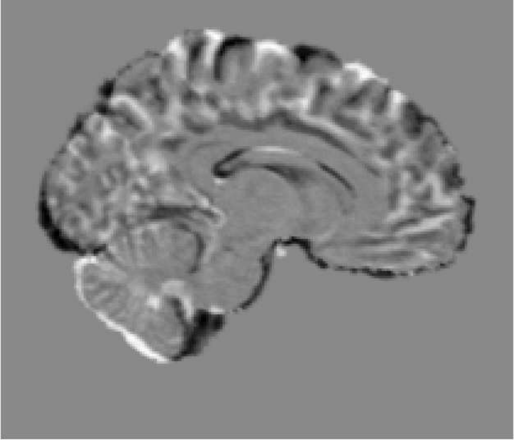Figure 2 shows the $MSE_{rel}$ and $\|g\|_{\infty,{rel}}$ convergence curves obtained during the optimization for band sizes of 16, 32, 40, 48, 56 and 64. The figure shows that both methods converge to similar $MSE_{rel}$ values. However, Jacobi PDE-LDDMM subject to the deformation state equation shows smaller $\|g\|_{\infty,{rel}}$ , which indicates a better convergence behavior. Table 1 shows the numeric values after 10 iterations. For BL sizes of 32 both methods achieve acceptable $MSE_{rel}$ values. Jacobi PDE-LDDMM subject to the deformation state equation slightly outperformed the method subject to the state equation.

Figure 2: Relative MSE and gradient convergence curves for the different band sizes.

	BL Jacobi PDE-LDDMM		BL Jacobi PDE-LDDMM
	s.t. state eq.		s.t. def. state eq.
BL size	$MSE_{rel}$	$\\|g\\|_{\infty,{rel}}$	$MSE_{rel}$	$\\|g\\|_{\infty,{rel}}$
16	21.41	0.03	21.29	0.03
32	16.56	0.01	15.90	0.03
40	15.45	0.02	14.92	0.03
48	12.10	0.03	14.47	0.03
56	13.48	0.03	14.26	0.03
64	14.74	0.02	14.16	0.03

Table 1: Relative MSE and gradient achieved by the proposed methods for the different band sizes.

Figure 3 shows the deformed images and the differences after registration. In the figure, it can be appreciated the accuracy achieved by the proposed methods. The difference between the deformed images is hardly perceptible.

Finally, Table 2 shows the VRAM memory load and the computation time exhibit by the proposed methods. It should be noticed that Jacobi PDE-LDDMM subject to the state equation in the spatial domain did not fit the memory of our available graphics card (11 GBs) and the computation time for a downsampled example of our data was 1825.50 seconds. Therefore, the band limited vector field parameterization definitively shows up a considerable computational saving.

	BL Jacobi PDE-LDDMM s.t. state eq.		BL Jacobi PDE-LDDMM s.t. def. state eq.
BL size	VRAM (MBS)	total time (s)	VRAM (MBS)	total time (s)
16	3319	892.56	1745	694.43
32	3439	894.38	1927	701.14
40	3579	845.57	2137	653.20
48	3803	869.67	2469	693.83
56	4097	1154.58	2907	1022.55
64	4403	1576.76	3393	1492.98

Table 2: Computational complexity of the proposed methods.

Acknowledgements

This work was partially supported by Spanish research grant TIN2016-80347-R.

References

[1] Sotiras, A., Davatzikos, C., Paragios, N.: Deformable medical image registration: A survey. IEEE Trans. Med. Imaging 32(7) (2013) 1153 – 1190
[2] Miller, M.I.: Computational anatomy: shape, growth, and atrophy comparison via diffeomorphisms. Neuroimage 23 (2004) 19–33
[3] Hart, G.L., Zach, C., Niethammer, M.: An optimal control approach for deformable registration. Proc. of the IEEE Conference on Computer Vision and Pattern Recognition (CVPR’09) (2009)
[4] Beg, M.F., Miller, M.I., Trouve, A., Younes, L.: Computing large deformation metric mappings via geodesic flows of diffeomorphisms. Int. J. Comput. Vision 61 (2) (2005) 139–157
[5] Vialard, F.X., Risser, L., Rueckert, D., Holm, D.D.: Diffeomorphic atlas estimation using geodesic shooting on volumetric images. Annals of the BMVA 2012 (2012) 1 – 12
[6] Mang, A., Biros, G.: An inexact Newton-Krylov algorithm for constrained diffeomorphic image registration. SIAM J. Imaging Sciences 8(2) (2015) 1030–1069
[7] Hernandez, M.: PDE-constrained LDDMM via geodesic shooting and inexact Gauss-Newton-Krylov optimization using the incremental adjoint Jacobi equations. ArXiv:1807.04638 (2018)
[8] Hernandez, M.: Band-Limited Stokes Large Deformation Diffeomorphic Metric Mapping. IEEE J. of Biom. and Health Inf. (2018)
[9] Hernandez, M.: Newton-Krylov PDE-constrained LDDMM in the space of band-limited vector fields. ArXiv:1807.05117 (2018)
[10] Holm, D.D., Marsden, J.E., Ratiu, T.S.: The Euler-Poincare equations and semidirect products with applications to continuum theories. Adv. in Math. 137 (1998) 1 – 81
[11] Younes, L.: Jacobi fields in groups of diffeomorphisms and applications. Q. Appl. Math. 65 (2007) 113 – 134
[12] Zhang, M., Fletcher, P.T.: Finite-dimensional Lie algebras for fast diffeomorphic image registration. Proc. of International Conference on Information Processing and Medical Imaging (IPMI’15), Lecture Notes in Computer Science (2015)
[13] Bullo, F.: Invariant affine connections and controllability on Lie groups. Techical report for Geometric Mechanics, California Institute of Technology (1995)
[14] Polzin, T., Niethammer, M., Heinrich, M.P., Handels, H., Modersitzki, J.: Memory efficient LDDMM for lung CT. (2014) 28–36

BL Jacobi subject to state equation

BL Jacobi subject to deformation state equation