跳到论文正文
W Papers独立论文阅读器 arXiv:1807.11232 论文正文 计算阅读时间 · 0%
引用这篇论文根据当前论文元数据生成,正式投稿前建议核对。


License: arXiv.org perpetual non-exclusive license
arXiv:1807.11232v1 [math.OC] 30 Jul 2018

An Approximate Newton Smoothing Method for Shape Optimization

Journal: arXiv
Jonas Kusch Corresponding author: Corresponding author Address: Karlsruhe Institute of Technology, Kaiserstr. 12, 76131 Karlsruhe, Germany    Stephan Schmidt Address: Universität Würzburg, Emil-Fischer-Str. 40, 97074 Würzburg, Germany    Nicolas R. Gauger Address: TU Kaiserslautern, Paul-Ehrlich-Str. 34, 67663 Kaiserslautern, Germany
Abstract

A novel methodology to efficiently approximate the Hessian for numerical shape optimization is considered. The method enhances operator symbol approximations by including body fitted coordinates and spatially changing symbols in a semi automated framework based on local Fourier analysis. Contrary to classical operator symbol methods, the proposed strategy will identify areas in which a non-smooth design is physically meaningful and will automatically turn off smoothing in these regions. A new strategy to also numerically identify the analytic symbol is derived, extending the procedure to a wide variety of problems. The effectiveness is demonstrated by using drag minimization in Stokes and Navier–Stokes flows.

Keywords:
shape optimization, smoothing, Hessian, Stokes, Navier-Stokes

1 Introduction

Shape optimization subject to partial differential equations plays an important role in a variety of problems such as minimum drag shapes in fluid dynamics, acoustics, material sciences or geometric inverse problems in non-destructive testing and medical imaging.

In order to propose an efficient design, an initial geometry is described with the help of a finite set of parameters, which are modified such that a given cost function is minimized. Steepest-descend methods iteratively modify the design according to the negative gradient with respect to the chosen parameters, thereby ensuring an successive descend of the cost function. The use of the adjoint approach [1] makes computing the gradient independent of the number of design parameters, promoting using all mesh node positions as design parameters, i.e., the richest design space possible. A downside of the plethora of design variables are possibly high-frequency oscillations in the search direction as no boundary smoothness is inherent in the parametrization. Consequently, resulting non-smooth designs can cause an irregular computational mesh resulting in the failure of the optimization.

A natural choice to overcome these difficulties is using a smoothed [1, 2, 3] or, equivalently, a Sobolev gradient descend [4], which necessitates a manual or automatic parameter study to determine a problem-dependent smoothing parameter [5]. Picking an adequate smoothing parameter is a crucial task as manipulating the search direction poorly can potentially slow down the convergence.

Additionally, the convergence speed of the steepest-Descent method deteriorates if the Hessian of the optimization problem is ill-conditioned [6, Chapter 3.3]. An approach to overcome the condition number dependency is Newton’s method, necessitating a computation of the Hessian. As it is computationally not feasible to determine the exact Hessian, a lot of work has gone into its approximation. One strategy is to approximate the symbol of the exact operator [7, 8, 9]. Furthermore, closely related studies based on Fourier analysis have also been used in [10] to study the condition of several Navier–Stokes flow situations, bridging the gap between optimization acceleration and studying the well- or ill-posed nature of flow problems.

An approach to construct a search direction fulfilling both, the desired regularity of the design as well as including Hessian information has been derived in [11] for energy minimization. The authors use the symbol of the exact Hessian for a half-space geometry to choose a constant parameter for Sobolev smoothing which is based on the spacing of the computational mesh. The choice of a constant smoothing parameter can however lead to a limitation of the design space, as non-smooth areas can become physically meaningful in certain areas of the design. One can for example think of the sharp trailing edge of an airfoil. Furthermore, the limitation to half-space geometries means that the smoothing parameter might not be valid in practical applications.

The aim of this paper is to extend the derivation of the Hessian symbol to body fitted coordinates, allowing the direct usage of the symbol in the construction of an approximate Newton method. The resulting preconditioner will inherit the local smoothing properties of the exact Hessian by picking spatially dependent smoothing parameters automatically. The paper is structured as follows: After the introduction in section 1, we derive the steepest-descent search direction in section 2. To accelerate the optimization, we derive the Hessian symbol in section 3 and discuss why the Hessian has smoothing behavior. This behavior is demonstrated and investigated further in section 4, where a numerical approximation of the Hessian symbol for low Reynolds number flows is presented. The considered technique to approximate this symbol gives insight into the smoothing properties of the Hessian. Having derived the analytic symbol, we construct a preconditioner, which approximates this symbol in section 5. To ensure minimal computational costs, we use differential operators to construct said preconditioner. The coefficients of these operators are determined automatically to match the exact Hessian symbol. Finally, we compare our novel method in section 6 to classical Sobolev smoothing when using a constant smoothing parameter.

2 The steepest-descent search direction

We start by defining the shape optimization problem for a general cost function FF given a Stokes flow: This constraint optimization problem takes the form

min𝒗,p,Γo⁡F⁡(𝒗,pCLOSE,\displaystyle\min_{\bm{v},p,\Gamma_{o}}F(\bm{v},p, OPENΓo)\displaystyle\Gamma_{o}) (1a)
s.t. −μ​Δ​𝒗+∇p\displaystyle\text{s.t. }-\mu\Delta\bm{v}+\nabla p =0,\displaystyle=0, (1b)
∇⋅𝒗\displaystyle\nabla\cdot\bm{v} =0,\displaystyle=0, (1c)
𝒗=0\displaystyle\bm{v}=0 on ​Γo,\displaystyle\text{ on }\Gamma_{o}, (1d)

where the design variable Γo\Gamma_{o} is the surface of a flow obstacle with volume Ωo\Omega_{o}. In our setting, the flow domain is given by Ω=ℝd∖Ωo\Omega=\mathbb{R}^{d}\setminus\Omega_{o}. The velocity 𝒗∈ℝ2\bm{v}\in\mathbb{R}^{2} and the pressure p∈ℝp\in\mathbb{R} fulfill the Stokes equations with dynamic viscosity μ\mu. Physically, the Stokes equations describe a creeping flow, in which convective forces are negligible compared to viscous forces. We are interested in the minimization of the obstacle’s drag, which is given by

FD:=∫Γo−μ(𝒏⋅∇)𝒗⋅𝒂+p𝒏⋅𝒂dΓ,F_{D}:=\int_{\Gamma_{o}}-\mu(\bm{n}\cdot\nabla)\bm{v}\cdot\bm{a}+p\bm{n}\cdot\bm{a}d\Gamma, (2)

where 𝒂\bm{a} is defined as

𝒂:=(cos⁡(ϕ),sin⁡(ϕ))T.\displaystyle\bm{a}:=(\cos(\phi),\sin(\phi))^{T}.

The angle of attack ϕ\phi will be zero in our case. Making use of gradient-based methods, the design variable Γo\Gamma_{o} is modified iteratively such that the cost function FDF_{D} is minimized. In order to calculate the gradient of the optimization problem (1), the shape derivative of the cost function needs to be determined. As proposed in [12, 13], the shape derivative can be computed by defining a mapping Tt​[𝑽]T_{t}[\bm{V}] which maps the original domain Ω\Omega to the deformed domain Ωt\Omega_{t}, given by

Tt​[𝑽]​(𝒙)=𝒙+t​𝑽​(𝒙).\displaystyle T_{t}[\bm{V}](\bm{x})=\bm{x}+t\bm{V}(\bm{x}).

The shape derivative of the cost function FF in the direction of the vector field 𝑽\bm{V} is then given by

d​F​(Ω)​[𝑽]:=dd​t|t=0​F​(Tt​[𝑽]​(Ω)).\displaystyle dF(\Omega)[\bm{V}]:=\left.\frac{d}{dt}\right|_{t=0}F(T_{t}[\bm{V}](\Omega)).

To efficiently calculate the shape derivative, one often makes use of the adjoint approach, which yields the following theorem:

Theorem 1

The shape derivative of problem (1) with respect to 𝐕\bm{V} using the drag (2) as cost function is

dFD(𝒗,p,Ω)[𝑽]=−∫Γo(𝑽⋅𝒏)[∑i=1dμ(𝒏⋅∇)λi(𝒏⋅∇)vi]dΓ\displaystyle dF_{D}(\bm{v},p,\Omega)[\bm{V}]=-\int_{\Gamma_{o}}(\bm{V}\cdot\bm{n})\left[\sum_{i=1}^{d}\mu(\bm{n}\cdot\nabla)\lambda_{i}(\bm{n}\cdot\nabla)v_{i}\right]d\Gamma

where the adjoint velocity 𝛌∈ℝd\bm{\lambda}\in\mathbb{R}^{d} is given by

−μ​Δ​𝝀−∇λp\displaystyle-\mu\Delta\bm{\lambda}-\nabla\lambda_{p} =𝟎,\displaystyle=\bm{0},
div⁡𝝀\displaystyle\div{\bm{\lambda}} =0,\displaystyle=0,
𝝀=−𝒂\displaystyle\bm{\lambda}=-\bm{a} on ​Γo\displaystyle\text{ on }\Gamma_{o}

and 𝐧\bm{n} is the normal vector of the optimization patch Γo\Gamma_{o}.

We start by calculating the shape derivative for a general cost function

F(𝒗,p,Γo)=∫Γof(𝒗,(𝒏⋅∇)𝒗,p,𝒏)dΓ.\displaystyle F(\bm{v},p,\Gamma_{o})=\int_{\Gamma_{o}}f(\bm{v},(\bm{n}\cdot\nabla)\bm{v},p,\bm{n})d\Gamma.

Following [14], the shape derivative of this cost function is

d​F​(Ω)​[𝑽]=\displaystyle dF(\Omega)[\bm{V}]= ∫Γo(𝑽⋅𝒏)[(𝒏⋅∇)f+κf]+∂f∂𝒏d𝒏[𝑽]dΓ\displaystyle\int_{\Gamma_{o}}(\bm{V}\cdot\bm{n})\left[(\bm{n}\cdot\nabla)f+\kappa f\right]+\frac{\partial f}{\partial\bm{n}}d\bm{n}[\bm{V}]d\Gamma
+∫Γo∂f∂vivi′[𝑽]+∂f∂bi(𝒏⋅∇)vi′[𝑽]+∂f∂pp′[𝑽]dΓ\displaystyle+\int_{\Gamma_{o}}\frac{\partial f}{\partial v_{i}}v_{i}^{\prime}[\bm{V}]+\frac{\partial f}{\partial b_{i}}(\bm{n}\cdot\bm{\nabla})v_{i}^{\prime}[\bm{V}]+\frac{\partial f}{\partial p}p^{\prime}[\bm{V}]d\Gamma

where 𝒃:=(𝒏⋅∇)𝒗\bm{b}:=(\bm{n}\cdot\nabla)\bm{v}, the curvature is denoted by κ\kappa and the tangential divergence of a vector field 𝑾\bm{W} is given by

divΓ(𝐖)=div(𝐖)−(𝐧⋅∇)𝐖⋅𝐧=∂xjWj−nk∂xkWjnj.\displaystyle\tandiv(\bm{W})=\div(\bm{W})-(\bm{n}\cdot\nabla)\bm{W}\cdot\bm{n}=\partial_{x_{j}}W_{j}-n_{k}\partial_{x_{k}}W_{j}n_{j}.

Furthermore, the normal derivative (𝒏⋅∇)(\bm{n}\cdot\nabla) is only applied to the first three inputs of ff, namely 𝒗,𝒃\bm{v},\bm{b} and pp. The gradient can be rewritten as

d​F​(Ω)​[𝑽]=\displaystyle dF(\Omega)[\bm{V}]= ∫Γo(𝑽⋅𝒏)[(𝒏⋅∇)f+κ(f−𝒏⋅∂f∂𝒏)+divΓ∂f∂𝐧]dΓ\displaystyle\int_{\Gamma_{o}}(\bm{V}\cdot\bm{n})\left[(\bm{n}\cdot\nabla)f+\kappa\left(f-\bm{n}\cdot\frac{\partial f}{\partial\bm{n}}\right)+\tandiv{\frac{\partial f}{\partial\bm{n}}}\right]d\Gamma
+∫Γo∂f∂vivi′[𝑽]+∂f∂bi(𝒏⋅∇)vi′[𝑽]+∂f∂pp′[𝑽]dΓ.\displaystyle+\int_{\Gamma_{o}}\frac{\partial f}{\partial v_{i}}v_{i}^{\prime}[\bm{V}]+\frac{\partial f}{\partial b_{i}}(\bm{n}\cdot\bm{\nabla})v_{i}^{\prime}[\bm{V}]+\frac{\partial f}{\partial p}p^{\prime}[\bm{V}]d\Gamma. (3)

The local shape derivative of the velocity and pressure due to a perturbation 𝑽\bm{V} is denoted by 𝒗′​[𝑽]\bm{v}^{\prime}[\bm{V}] and p′​[𝑽]p^{\prime}[\bm{V}]. Computing these two functions is numerically expensive, which is why we aim at finding a representation of the shape derivative, independent of these two terms. The functions 𝒗′​[𝑽]\bm{v}^{\prime}[\bm{V}] and p′​[𝑽]p^{\prime}[\bm{V}] are determined by linearizing the Stokes equations around the primal state 𝒗\bm{v} and pp, meaning that we write down the Stokes equation for the states of the perturbed geometry with 𝒗~=𝒗+𝒗′\bm{\tilde{v}}=\bm{v}+\bm{v^{\prime}} and p~=p+p′\tilde{p}=p+p^{\prime}. This yields

−μ​Δ​𝒗′​[𝑽]+∇p′​[𝑽]\displaystyle-\mu\Delta\bm{v}^{\prime}[\bm{V}]+\nabla p^{\prime}[\bm{V}] =0,\displaystyle=0, (4a)
∇⋅𝒗′​[𝑽]\displaystyle\nabla\cdot\bm{v}^{\prime}[\bm{V}] =0,\displaystyle=0, (4b)
𝒗′[𝑽]=−(𝒏⋅∇)𝒗(𝒏\displaystyle\bm{v}^{\prime}[\bm{V}]=-(\bm{n}\cdot\nabla)\bm{v}(\bm{n} ⋅𝑽) on Γo.\displaystyle\cdot\bm{V})\text{ on }\Gamma_{o}. (4c)

The derivation of the boundary condition can be performed by a Taylor expansion. For more details see [14]. In order to eliminate the velocity and pressure perturbations 𝒗′\bm{v}^{\prime} and p′p^{\prime} in the shape derivative (3), one chooses the adjoint ansatz. We start by taking the integral of the scalar product of the linearized Stokes equations (4) and the adjoint states (𝝀,λp)T(\bm{\lambda},\lambda_{p})^{T}, where 𝝀∈ℝd\bm{\lambda}\in\mathbb{R}^{d} is the adjoint velocity and λp\lambda_{p} is the adjoint pressure, leading to

0=∫Ω−λkμ∂xj​xjvk′+λk∂xkp′+λp∂xkvk′dΩ.0=\int_{\Omega}-\lambda_{k}\mu\partial_{x_{j}x_{j}}v_{k}^{\prime}+\lambda_{k}\partial_{x_{k}}p^{\prime}+\lambda_{p}\partial_{x_{k}}v_{k}^{\prime}d\Omega. (5)

Let us look at each term of the adjoint part individually. We start with

∫Ω−λkμ∂xj​xjvk′dΩ=\displaystyle\int_{\Omega}-\lambda_{k}\mu\partial_{x_{j}x_{j}}v_{k}^{\prime}d\Omega= ∫Ω−μ∂xj(λk∂xjvk′)+μ∂xjλk∂xjvk′dΩ\displaystyle\int_{\Omega}-\mu\partial_{x_{j}}(\lambda_{k}\partial_{x_{j}}v_{k}^{\prime})+\mu\partial_{x_{j}}\lambda_{k}\partial_{x_{j}}v_{k}^{\prime}d\Omega
=\displaystyle= ∫Γo−μnjλk∂xjvk′dΓ+∫Ωμ∂xj(vk′∂xjλk)−μvk′∂xj​xjλkdΩ\displaystyle\int_{\Gamma_{o}}-\mu n_{j}\lambda_{k}\partial_{x_{j}}v_{k}^{\prime}d\Gamma+\int_{\Omega}\mu\partial_{x_{j}}\left(v_{k}^{\prime}\partial_{x_{j}}\lambda_{k}\right)-\mu v_{k}^{\prime}\partial_{x_{j}x_{j}}\lambda_{k}d\Omega
=\displaystyle= ∫Γo−njμλk∂xjvk′dΓ+∫Γoμnjvk′∂xjλk−∫Ωμvk′∂xj​xjλkdΩ.\displaystyle\int_{\Gamma_{o}}-n_{j}\mu\lambda_{k}\partial_{x_{j}}v_{k}^{\prime}d\Gamma+\int_{\Gamma_{o}}\mu n_{j}v_{k}^{\prime}\partial_{x_{j}}\lambda_{k}-\int_{\Omega}\mu v_{k}^{\prime}\partial_{x_{j}x_{j}}\lambda_{k}d\Omega.

Here, we used the reverse chain rule as well as Gauss divergence theorem. The remaining two terms can be transformed with the same strategy. We obtain

∫Ωλk∂xkp′dΩ=−∫Ωp′∂xkλkdΩ+∫Γonkλkp′dΓ,\displaystyle\int_{\Omega}\lambda_{k}\partial_{x_{k}}p^{\prime}d\Omega=-\int_{\Omega}p^{\prime}\partial_{x_{k}}\lambda_{k}d\Omega+\int_{\Gamma_{o}}n_{k}\lambda_{k}p^{\prime}d\Gamma,
∫Ωλp∂xkvk′dΩ=−∫Ωvk′∂xkλpdΩ+∫Γoλpvk′nkdΓ.\displaystyle\int_{\Omega}\lambda_{p}\partial_{x_{k}}v_{k}^{\prime}d\Omega=-\int_{\Omega}v_{k}^{\prime}\partial_{x_{k}}\lambda_{p}d\Omega+\int_{\Gamma_{o}}\lambda_{p}v_{k}^{\prime}n_{k}d\Gamma.

Adding the transformed equation (5) to the gradient (3), we get

d​F​(Ω)​[𝑽]+0=\displaystyle dF(\Omega)[\bm{V}]+0= ∫ΓoVl​nl​[nj​∂xjf+κ⁡(f−nj​∂f∂nj)+divΓ⁡∂f∂nj]​𝑑Γ\displaystyle\int_{\Gamma_{o}}V_{l}n_{l}\left[n_{j}\partial_{x_{j}}f+\kappa\left(f-n_{j}\frac{\partial f}{\partial n_{j}}\right)+\tandiv{\frac{\partial f}{\partial n_{j}}}\right]d\Gamma
+∫Γo∂f∂vjvj′+∂f∂bj(nk∂xk)vj′+∂f∂pp′dΓ\displaystyle+\int_{\Gamma_{o}}\frac{\partial f}{\partial v_{j}}v_{j}^{\prime}+\frac{\partial f}{\partial b_{j}}(n_{k}\partial_{x_{k}})v_{j}^{\prime}+\frac{\partial f}{\partial p}p^{\prime}d\Gamma
+∫Γo−μλjnk∂xkvj′+μnkvj′∂xkλj+njλjp′+λpvj′njdΓ\displaystyle+\int_{\Gamma_{o}}-\mu\lambda_{j}n_{k}\partial_{x_{k}}v_{j}^{\prime}+\mu n_{k}v_{j}^{\prime}\partial_{x_{k}}\lambda_{j}+n_{j}\lambda_{j}p^{\prime}+\lambda_{p}v_{j}^{\prime}n_{j}d\Gamma
+∫Ω−μvk′∂xj​xjλk−p′∂xkλk−vk′∂xkλpdΩ.\displaystyle+\int_{\Omega}-\mu v_{k}^{\prime}\partial_{x_{j}x_{j}}\lambda_{k}-p^{\prime}\partial_{x_{k}}\lambda_{k}-v_{k}^{\prime}\partial_{x_{k}}\lambda_{p}d\Omega. (6)

Remembering that the adjoint states (𝝀,λp)T(\bm{\lambda},\lambda_{p})^{T} are still free to choose, those states can be picked to cancel the perturbations of the primal states. The resulting constraint for the adjoint states is called the adjoint equation. By looking at the volume part of the gradient (6), we see that in Ω\Omega we must have

−μ​Δ​𝝀−∇λp\displaystyle-\mu\Delta\bm{\lambda}-\nabla\lambda_{p} =𝟎,\displaystyle=\bm{0},
div⁡𝝀\displaystyle\div{\bm{\lambda}} =0.\displaystyle=0.

Now, let us determine the adjoint boundary conditions, i.e. the conditions, which the adjoint states must fulfill on the boundaries such that the perturbed primal states drop out of the gradient (6). Assuming that we fulfill the adjoint equations, we can rearrange the gradient to

d​F​(Ω)​[𝑽]=\displaystyle dF(\Omega)[\bm{V}]= ∫ΓoVl​nl​[nj​∂xjf+κ⁡(f−nj​∂f∂nj)+divΓ⁡∂f∂nj]​𝑑Γ\displaystyle\int_{\Gamma_{o}}V_{l}n_{l}\left[n_{j}\partial_{x_{j}}f+\kappa\left(f-n_{j}\frac{\partial f}{\partial n_{j}}\right)+\tandiv{\frac{\partial f}{\partial n_{j}}}\right]d\Gamma
+∫Γovj′[∂f∂vj+μnk∂xkλj+λpnj]+(nk∂xk)vj′[∂f∂bj−μλj]+p′[∂f∂p+njλj]dΓ.\displaystyle+\int_{\Gamma_{o}}v_{j}^{\prime}\left[\frac{\partial f}{\partial v_{j}}+\mu n_{k}\partial_{x_{k}}\lambda_{j}+\lambda_{p}n_{j}\right]+(n_{k}\partial_{x_{k}})v_{j}^{\prime}\left[\frac{\partial f}{\partial b_{j}}-\mu\lambda_{j}\right]+p^{\prime}\left[\frac{\partial f}{\partial p}+n_{j}\lambda_{j}\right]d\Gamma.

Remember that we have vj′=Vlnl(ni∂xi)vjv_{j}^{\prime}=V_{l}n_{l}(n_{i}\partial_{x_{i}})v_{j} on Γo\Gamma_{o} from the boundary conditions of the linearized Stokes equations (4), which is why we do not need to calculate vj′v_{j}^{\prime}. The remaining perturbed primal states are forced to vanish with the help of the adjoint boundary conditions. Hence, on Γo\Gamma_{o} the adjoint states must fulfill

∂f∂𝒃−μ​𝝀=𝟎,\displaystyle\frac{\partial f}{\partial\bm{b}}-\mu\bm{\lambda}=\bm{0}, (8a)
∂f∂p+𝒏⋅𝝀=0.\displaystyle\frac{\partial f}{\partial p}+\bm{n}\cdot\bm{\lambda}=0. (8b)

If the dual states fulfill these conditions, we are left with

d​F​(Ω)​[𝑽]=\displaystyle dF(\Omega)[\bm{V}]= ∫ΓoVl​nl​[nj​∂xjf+κ⁡(f−nj​∂f∂nj)+divΓ⁡∂f∂nj]​𝑑Γ\displaystyle\int_{\Gamma_{o}}V_{l}n_{l}\left[n_{j}\partial_{x_{j}}f+\kappa\left(f-n_{j}\frac{\partial f}{\partial n_{j}}\right)+\tandiv{\frac{\partial f}{\partial n_{j}}}\right]d\Gamma
+∫ΓoVlnl(ni∂xi)vj[∂f∂vj+μnk∂xkλj+λpnj]dΓ.\displaystyle+\int_{\Gamma_{o}}V_{l}n_{l}(n_{i}\partial_{x_{i}})v_{j}\left[\frac{\partial f}{\partial v_{j}}+\mu n_{k}\partial_{x_{k}}\lambda_{j}+\lambda_{p}n_{j}\right]d\Gamma.

Let us now simplify the gradient (6) as well as the adjoint boundary conditions (8) for the drag minimization problem by making use of

fD=−μ𝒃⋅𝒂+p𝒏⋅𝒂.\displaystyle f_{D}=-\mu\bm{b}\cdot\bm{a}+p\bm{n}\cdot\bm{a}.

We have

∂fD∂𝒗\displaystyle\frac{\partial f_{D}}{\partial\bm{v}} =𝟎​,​∂fD∂𝒃=−μ​𝒂,\displaystyle=\bm{0}\text{,}\enskip\frac{\partial f_{D}}{\partial\bm{b}}=-\mu\bm{a},
∂fD∂p\displaystyle\frac{\partial f_{D}}{\partial p} =𝒏⋅𝒂,∂fD∂𝒏=−μ∇𝒗⋅𝒂+p𝒂.\displaystyle=\bm{n}\cdot\bm{a},\enskip\frac{\partial f_{D}}{\partial\bm{n}}=-\mu\nabla\bm{v}\cdot\bm{a}+p\bm{a}.

Hence, the adjoint boundary conditions on Γo\Gamma_{o} become 𝝀=−𝒂\bm{\lambda}=-\bm{a}. Furthermore, the gradient changes to

dFD(Ω)[𝑽]=∫ΓoVlnl[nj∂xjfD+divΓ∂fD∂nj]+Vlnl(ni∂xi)vj[μnk∂xkλj+λpnj]dΓ,\displaystyle dF_{D}(\Omega)[\bm{V}]=\int_{\Gamma_{o}}V_{l}n_{l}\left[n_{j}\partial_{x_{j}}f_{D}+\tandiv{\frac{\partial f_{D}}{\partial n_{j}}}\right]+V_{l}n_{l}(n_{i}\partial_{x_{i}})v_{j}\left[\mu n_{k}\partial_{x_{k}}\lambda_{j}+\lambda_{p}n_{j}\right]d\Gamma,

because fDf_{D} is linear in the nn argument and consequently

fD−𝒏​∂fD∂𝒏=0.\displaystyle f_{D}-\bm{n}\frac{\partial f_{D}}{\partial\bm{n}}=0.

Additionally, the term Vlnl(ni∂xi)vjλpnjV_{l}n_{l}(n_{i}\partial_{x_{i}})v_{j}\lambda_{p}n_{j} is zero, because we can rewrite the velocity gradient as

∂xjvl=ni​∂xivl​nj+tk​∂xkvl​tj.\displaystyle\partial_{x_{j}}v_{l}=n_{i}\partial_{x_{i}}v_{l}n_{j}+t_{k}\partial_{x_{k}}v_{l}t_{j}.

Due to the no-slip boundary condition, the derivative w.r.t. the tangential direction 𝒕\bm{t} drops out. If we now choose the resulting gradient to write down the mass conservation, we get

∂xjvj=ni​∂xivj​nj=0.\displaystyle\partial_{x_{j}}v_{j}=n_{i}\partial_{x_{i}}v_{j}n_{j}=0.

Plugging in the remaining derivatives of fDf_{D}, we are left with

dFD(Ω)[𝑽]=∫Γo\displaystyle dF_{D}(\Omega)[\bm{V}]=\int_{\Gamma_{o}} Vlnl[nj∂xj(−μnk∂xkviai+pnkak)+divΓ(−μ∂xjvkak+paj)]\displaystyle V_{l}n_{l}\left[n_{j}\partial_{x_{j}}\left(-\mu n_{k}\partial_{x_{k}}v_{i}a_{i}+pn_{k}a_{k}\right)+\tandiv\left(-\mu\partial_{x_{j}}v_{k}a_{k}+pa_{j}\right)\right]
+\displaystyle+ Vlnl(ni∂xi)vjμnk∂xkλjdΓ\displaystyle V_{l}n_{l}(n_{i}\partial_{x_{i}})v_{j}\mu n_{k}\partial_{x_{k}}\lambda_{j}d\Gamma
=∫Γo\displaystyle=\int_{\Gamma_{o}} (𝑽⋅𝒏)[−μ(∇𝒏)2𝒗𝒂+(𝒏⋅∇)p(𝒏⋅𝒂)−divΓ(−μ(∇𝒗)T𝒂+p𝒂)]\displaystyle(\bm{V}\cdot\bm{n})\left[-\mu(\nabla_{\bm{n}})^{2}\bm{v}\bm{a}+(\bm{n}\cdot\nabla)p(\bm{n}\cdot\bm{a})-\div_{\Gamma}(-\mu(\nabla\bm{v})^{T}\bm{a}+p\bm{a})\right]
+\displaystyle+ (𝑽⋅𝒏)[μ(𝒏⋅∇)λi(𝒏⋅∇)vi]dΓ,\displaystyle(\bm{V}\cdot\bm{n})\left[\mu(\bm{n}\cdot\nabla)\lambda_{i}(\bm{n}\cdot\nabla)v_{i}\right]d\Gamma, (9)

where we have used

(∇𝒏)2​𝒗:=nj​∂xj(nk​∂xkvi).\displaystyle(\nabla_{\bm{n}})^{2}\bm{v}:=n_{j}\partial_{x_{j}}\left(n_{k}\partial_{x_{k}}v_{i}\right).

The derived shape derivative can further be simplified to facilitate the derivation of the Hessian: Taking a closer look at the tangential divergence part of (9), one sees that the term inside the tangential divergence becomes

divΓ(−μ∇𝒗⋅𝒂)\displaystyle\div_{\Gamma}(-\mu\nabla\bm{v}\cdot\bm{a}) =div(−μ∇𝒗⋅𝒂)−𝒏⋅∇(−μ∇𝒗⋅𝒂)⋅𝒏\displaystyle=\div(-\mu\nabla\bm{v}\cdot\bm{a})-\bm{n}\cdot\nabla(-\mu\nabla\bm{v}\cdot\bm{a})\cdot\bm{n}
=−∂xj(μ∂xjvkak)+μni∂xi(∂xjvkak)nj\displaystyle=-\partial_{x_{j}}(\mu\partial_{x_{j}}v_{k}a_{k})+\mu n_{i}\partial_{x_{i}}(\partial_{x_{j}}v_{k}a_{k})n_{j}
=−μ∂xj​xjvkak+μni∂xi​xjvkaknj.\displaystyle=-\mu\partial_{x_{j}x_{j}}v_{k}a_{k}+\mu n_{i}\partial_{x_{i}x_{j}}v_{k}a_{k}n_{j}.

For the remaining term, we get

divΓ⁡(p​𝒂)\displaystyle\div_{\Gamma}(p\bm{a}) =div(p𝒂)−(𝒏⋅∇)(p𝒂)⋅𝒏\displaystyle=\div(p\bm{a})-(\bm{n}\cdot\nabla)(p\bm{a})\cdot\bm{n}
=∂xjp​aj−nk​∂xkp​aj​nj.\displaystyle=\partial_{x_{j}}pa_{j}-n_{k}\partial_{x_{k}}pa_{j}n_{j}.

Hence, the tangential divergence term in (9) becomes

∫Γo(Vlnl)[−μ∂xj​xjvkak+μni∂xi​xjvkaknj+∂xjpaj−nk∂xkpajnj]dΓ\displaystyle\int_{\Gamma_{o}}(V_{l}n_{l})\left[-\mu\partial_{x_{j}x_{j}}v_{k}a_{k}+\mu n_{i}\partial_{x_{i}x_{j}}v_{k}a_{k}n_{j}+\partial_{x_{j}}pa_{j}-n_{k}\partial_{x_{k}}pa_{j}n_{j}\right]d\Gamma
=\displaystyle= ∫Γo(𝑽⋅𝒏)[−μΔ𝒗⋅𝒂+μ(∇𝒏)2𝒗𝒂+∇p⋅𝒂−(𝒏⋅∇)p(𝒏⋅𝒂)]dΓ\displaystyle\int_{\Gamma_{o}}(\bm{V}\cdot\bm{n})\left[-\mu\Delta\bm{v}\cdot\bm{a}+\mu(\nabla_{\bm{n}})^{2}\bm{v}\bm{a}+\nabla p\cdot\bm{a}-(\bm{n}\cdot\nabla)p(\bm{n}\cdot\bm{a})\right]d\Gamma
=\displaystyle= ∫Γo(𝑽⋅𝒏)[(−μΔ𝒗+∇p)⋅𝒂+μ(∇𝒏)2𝒗𝒂−(𝒏⋅∇)p(𝒏⋅𝒂)]dΓ\displaystyle\int_{\Gamma_{o}}(\bm{V}\cdot\bm{n})\left[(-\mu\Delta\bm{v}+\nabla p)\cdot\bm{a}+\mu(\nabla_{\bm{n}})^{2}\bm{v}\bm{a}-(\bm{n}\cdot\nabla)p(\bm{n}\cdot\bm{a})\right]d\Gamma
=\displaystyle= ∫Γo(𝑽⋅𝒏)[μ(∇𝒏)2𝒗𝒂−(𝒏⋅∇)p(𝒏⋅𝒂)]dΓ.\displaystyle\int_{\Gamma_{o}}(\bm{V}\cdot\bm{n})\left[\mu(\nabla_{\bm{n}})^{2}\bm{v}\bm{a}-(\bm{n}\cdot\nabla)p(\bm{n}\cdot\bm{a})\right]d\Gamma.

Note, that −μ​Δ​𝒗+∇p-\mu\Delta\bm{v}+\nabla p is zero, due to the fact that the state variables fulfill the Stokes equations. Now most of the terms in (9) cancel, meaning that we are left with

d​FD​(Ω)​[𝑽]=∫Γo(𝑽⋅𝒏)​d​fD​𝑑Γ\displaystyle dF_{D}(\Omega)[\bm{V}]=\int_{\Gamma_{o}}(\bm{V}\cdot\bm{n})df_{D}d\Gamma

where

dfD:=−∑i=1dμ(𝒏⋅∇)λi(𝒏⋅∇)vi.\displaystyle df_{D}:=-\sum_{i=1}^{d}\mu(\bm{n}\cdot\nabla)\lambda_{i}(\bm{n}\cdot\nabla)v_{i}. (10)

∎With the help of the adjoint approach, a numerically cheap calculation of the shape derivative can be ensured, as the computational costs no longer depend on the number of design parameters. This motivates using a detailed description of the optimization patch Γo\Gamma_{o} by using the nodes of the discretized surface, defined by 𝒙k\bm{x}_{k} for k=1,…,Nk=1,...,N as design parameters. Having derived the shape derivative of the optimization problem (1), one can iteratively approach the optimal design with a steepest-descent update. To obtain a search direction for every surface node with the help of the shape derivative, the perturbations

𝑽k​(𝒙):=𝒏⁡(𝒙)​φk​(𝒙),\displaystyle\bm{V}_{k}(\bm{x}):=\bm{n}(\bm{x})\varphi_{k}(\bm{x}), (11)

for k=1,…,Nk=1,...,N is defined, where φk:Γo→ℝ\varphi_{k}:\Gamma_{o}\to\mathbb{R} are piece-wise linear basis functions fulfilling φk​(𝒙l)=1​ if ​𝒙l=𝒙k\varphi_{k}(\bm{x}_{l})=1\text{ if }\bm{x}_{l}=\bm{x}_{k}. The deformation of the kk-th mesh node is now given by

𝒙knew\displaystyle\bm{x}_{k}^{\text{new}} =𝒙k−𝑽k​(𝒙k)​d​FD​[𝑽k​(𝒙k)]\displaystyle=\bm{x}_{k}-\bm{V}_{k}(\bm{x}_{k})dF_{D}[\bm{V}_{k}(\bm{x}_{k})]
=𝒙k−𝒏⁡(𝒙k)​φk​(𝒙k)​d​FD​[𝒏⁡(𝒙k)​φk​(𝒙k)]\displaystyle=\bm{x}_{k}-\bm{n}(\bm{x}_{k})\varphi_{k}(\bm{x}_{k})dF_{D}[\bm{n}(\bm{x}_{k})\varphi_{k}(\bm{x}_{k})]
≈𝒙k−12​𝒏​(𝒙k)​d​fD​(𝒙k)​(‖𝒙k−𝒙k−1‖+‖𝒙k+1−𝒙k‖),\displaystyle\approx\bm{x}_{k}-\frac{1}{2}\bm{n}(\bm{x}_{k})df_{D}(\bm{x}_{k})\left(\|\bm{x}_{k}-\bm{x}_{k-1}\|+\|\bm{x}_{k+1}-\bm{x}_{k}\|\right),

where we used a first order quadrature rule to evaluate the integral in d​FDdF_{D}. Choosing an adequate step size γ\gamma yields the steepest-descent update

𝒙k(l+1)=𝒙k(l)+γ​pk(l)​𝒏​(xk(l)),\displaystyle\bm{x}_{k}^{(l+1)}=\bm{x}_{k}^{(l)}+\gamma p_{k}^{(l)}\bm{n}\left(x_{k}^{(l)}\right),

where the steepest-descent search direction is given by

pk(l)=−d​fD​(𝒙k(l)).\displaystyle p_{k}^{(l)}=-df_{D}\left(\bm{x}_{k}^{(l)}\right).

Alternatively, we can collect all values of the gradient evaluated at the surface points in a vector

𝒅​𝒇(l)=(d​fD​(𝒙1(l)),⋯,d​fD​(𝒙N(l)))T,\displaystyle\bm{df}^{(l)}=\left(df_{D}\left(\bm{x}_{1}^{(l)}\right),\cdots,df_{D}\left(\bm{x}_{N}^{(l)}\right)\right)^{T}, (12)

yielding the steepest-descent search direction

𝒑(l)=−𝒅​𝒇(l).\displaystyle\bm{p}^{(l)}=-\bm{df}^{(l)}.

As already discussed, the convergence of steepest-descent is slow. Additionally, the gradient d​fDdf_{D} is of insufficient regularity, leading to rough designs with subsequent problems in getting the flow solver to converge. To overcome this problem, we derive the Hessian of the optimization problem analytically. When given a Hessian matrix 𝑯∈ℝN×N\bm{H}\in\mathbb{R}^{N\times N}, we can choose the Newton search direction

𝒑(l)=−𝑯−1​𝒅​𝒇(l).\displaystyle\bm{p}^{(l)}=-\bm{H}^{-1}\bm{df}^{(l)}. (13)

The derivation of the Hessian will show that the inverse Hessian will have properties of a smoothing method, which is why we can combine the tasks of accelerating the optimization and smoothing the search direction.

3 The analytic Hessian symbol

In order to accelerate the optimization process, we wish to make use of Hessian information, or to be more precise, the symbol of the Hessian. This derivation uses the techniques introduced in [7, 8, 9, 11]. In contrast to previous works, our analysis holds for smooth geometries beyond the typical upper half-plane, allowing the derivation of the Hessian symbol in applications of practical interest. For a given operator LL, its symbol σL\sigma_{L} is the response of LL to a wave with a fixed frequency ω\omega. To give a brief understanding of operator symbols, we look at the following example:

We derive the symbol of the operator

L​g:=(1−d2d​x2)​g.\displaystyle Lg:=\left(1-\frac{d^{2}}{dx^{2}}\right)g.

To derive the response of LL to an input wave, we choose g=e−i​ω​xg=e^{-i\omega x}, which yields

L​e−i​ω​x=(1+ω2)​e−i​ω​x.\displaystyle Le^{-i\omega x}=\left(1+\omega^{2}\right)e^{-i\omega x}.

The symbol is therefore given by σL=1+ω2\sigma_{L}=1+\omega^{2}. It can be seen that the operator LL amplifies frequencies quadratically with respect to the input frequency ω\omega. The fact that σL\sigma_{L} is a real number, tells us that the operator does not cause a phase shift. Our aim is to derive the Hessian symbol σH\sigma_{H} for the drag minimization problem when using the Stokes equations. For this, the Hessian response to a Fourier mode with frequency ω\omega, which is used to perturb the optimization patch Γo\Gamma_{o} is investigated analytically. We assume a two-dimensional geometry, which can be described by body fitted coordinates ξ1\xi_{1} and ξ2\xi_{2}. A mapping to the physical coordinates is given by

Φ⁡(ξ1,ξ2)=𝒙.\displaystyle\Phi\left(\xi_{1},\xi_{2}\right)=\bm{x}.

The physical coordinates of the optimization patch are

Γo​(ξ1)=Φ⁡(ξ1,0),\displaystyle\Gamma_{o}(\xi_{1})=\Phi\left(\xi_{1},0\right),

meaning that ξ1\xi_{1} is the parameter describing the position on the optimization patch. We choose the parametrization such that

‖dd​ξ1​Γo​(ξ1)‖=1,\displaystyle\left\|\frac{d}{d\xi_{1}}\Gamma_{o}(\xi_{1})\right\|=1,

i.e., the tangential vector 𝒕\bm{t} has unit length. If the remaining parameter ξ2\xi_{2} is used as a parametrization into the normal direction 𝒏\bm{n}, we can write our mapping as

Φ⁡(ξ1,ξ2)=Γo​(ξ1)+ξ2​𝒏​(Γo​(ξ1)).\displaystyle\Phi\left(\xi_{1},\xi_{2}\right)=\Gamma_{o}(\xi_{1})+\xi_{2}\bm{n}(\Gamma_{o}(\xi_{1})).

In this setting, we derive the symbol of the Hessian in the following theorem.

Theorem 2

The symbol of the Hessian for the Stokes equations is given by

σH=β1+β2​ω\displaystyle\sigma_{H}=\beta_{1}+\beta_{2}\omega (14)

where

β1=μ(𝒏⋅∇)(∑k=12(𝒏⋅∇)vk(𝒏⋅∇)λk)\displaystyle\beta_{1}=\mu(\bm{n}\cdot\nabla)\left(\sum_{k=1}^{2}(\bm{n}\cdot\nabla)v_{k}(\bm{n}\cdot\nabla)\lambda_{k}\right) (15)

and

β2=−2μ∑k=12(𝒏⋅∇)λk(𝒏⋅∇)vk.\beta_{2}=-2\mu\sum_{k=1}^{2}(\bm{n}\cdot\nabla)\lambda_{k}(\bm{n}\cdot\nabla)v_{k}. (16)

The Hessian of our problem is the response of the gradient d​fDdf_{D} given in (10) to a perturbation of the design space, which we call α\alpha. The response of a function gg due to a perturbation α\alpha is denoted as

g′​[α]=limϵ→0g⁡(Γoϵ)−g⁡(Γo)ϵ,\displaystyle g^{\prime}[\alpha]=\lim_{\epsilon\rightarrow 0}\frac{g(\Gamma_{o}^{\epsilon})-g(\Gamma_{o})}{\epsilon},

where the perturbed surface is given by

Γoϵ:=Γo+ϵ​α​𝒏.\displaystyle\Gamma_{o}^{\epsilon}:=\Gamma_{o}+\epsilon\alpha\bm{n}.

The response of the gradient d​fDdf_{D} to such a perturbation is now given by

dfD′[α]=−μnk∂xkλi′[α]nl∂xlvi−μnk∂xkλinl∂xlvi′[α].df_{D}^{\prime}[\alpha]=-\mu n_{k}\partial_{x_{k}}\lambda_{i}^{\prime}[\alpha]n_{l}\partial_{x_{l}}v_{i}-\mu n_{k}\partial_{x_{k}}\lambda_{i}n_{l}\partial_{x_{l}}v_{i}^{\prime}[\alpha]. (17)

The change of the state variables as well as the adjoint variables due to a small perturbation α\alpha in the normal direction can be computed from the linearized primal and adjoint state equations, which are

−μ​Δ​𝒗′​[α]+∇p′​[α]\displaystyle-\mu\Delta\bm{v}^{\prime}[\alpha]+\nabla p^{\prime}[\alpha] =0,\displaystyle=0,
∇⋅𝒗′​[α]\displaystyle\nabla\cdot\bm{v}^{\prime}[\alpha] =0,\displaystyle=0,
𝒗′[α]=−(𝒏⋅∇)𝒗α on\displaystyle\bm{v}^{\prime}[\alpha]=-(\bm{n}\cdot\nabla)\bm{v}\alpha\text{ on } Γo,\displaystyle\Gamma_{o},

and

−μ​Δ​𝝀′​[α]−∇λp′​[α]\displaystyle-\mu\Delta\bm{\lambda}^{\prime}[\alpha]-\nabla\lambda_{p}^{\prime}[\alpha] =0,\displaystyle=0,
∇⋅𝝀′​[α]\displaystyle\nabla\cdot\bm{\lambda}^{\prime}[\alpha] =0,\displaystyle=0,
𝝀′[α]=−(𝒏⋅∇)𝝀α on\displaystyle\bm{\lambda}^{\prime}[\alpha]=-(\bm{n}\cdot\nabla)\bm{\lambda}\alpha\text{ on } Γo.\displaystyle\Gamma_{o}.

Transforming these equations into body fitted coordinates (ξ1,ξ2)(\xi_{1},\xi_{2}) leads to

−μ​∂ξl∂xi​∂2vj′​[α]∂ξk​ξl​∂ξk∂xi−μ​∂vj′∂ξk​∂2ξk∂xi2+∂p′​[α]∂ξk​∂ξk∂xj\displaystyle-\mu\frac{\partial\xi_{l}}{\partial x_{i}}\frac{\partial^{2}v_{j}^{\prime}[\alpha]}{\partial\xi_{k}\xi_{l}}\frac{\partial\xi_{k}}{\partial x_{i}}-\mu\frac{\partial v_{j}^{\prime}}{\partial\xi_{k}}\frac{\partial^{2}\xi_{k}}{\partial x_{i}^{2}}+\frac{\partial p^{\prime}[\alpha]}{\partial\xi_{k}}\frac{\partial\xi_{k}}{\partial x_{j}} =0,\displaystyle=0, (18a)
∂vi′​[α]∂ξk​∂ξk∂xi\displaystyle\frac{\partial v_{i}^{\prime}[\alpha]}{\partial\xi_{k}}\frac{\partial\xi_{k}}{\partial x_{i}} =0,\displaystyle=0, (18b)
vj′​[α]=−nk​∂vj∂ξi​∂ξi∂xk​α​ on\displaystyle v_{j}^{\prime}[\alpha]=-n_{k}\frac{\partial v_{j}}{\partial\xi_{i}}\frac{\partial\xi_{i}}{\partial x_{k}}\alpha\text{ on } Γo,\displaystyle\Gamma_{o}, (18c)

and

−μ​∂ξl∂xi​∂2λj′​[α]∂ξk​ξl​∂ξk∂xi−μ​∂λj′∂ξk​∂2ξk∂xi2−∂λp′​[α]∂ξk​∂ξk∂xj\displaystyle-\mu\frac{\partial\xi_{l}}{\partial x_{i}}\frac{\partial^{2}\lambda_{j}^{\prime}[\alpha]}{\partial\xi_{k}\xi_{l}}\frac{\partial\xi_{k}}{\partial x_{i}}-\mu\frac{\partial\lambda_{j}^{\prime}}{\partial\xi_{k}}\frac{\partial^{2}\xi_{k}}{\partial x_{i}^{2}}-\frac{\partial\lambda_{p}^{\prime}[\alpha]}{\partial\xi_{k}}\frac{\partial\xi_{k}}{\partial x_{j}} =0,\displaystyle=0, (19a)
∂λi′​[α]∂ξk​∂ξk∂xi\displaystyle\frac{\partial\lambda_{i}^{\prime}[\alpha]}{\partial\xi_{k}}\frac{\partial\xi_{k}}{\partial x_{i}} =0,\displaystyle=0, (19b)
λj′​[α]=−nk​∂λj∂ξi​∂ξi∂xk​α​ on\displaystyle\lambda_{j}^{\prime}[\alpha]=-n_{k}\frac{\partial\lambda_{j}}{\partial\xi_{i}}\frac{\partial\xi_{i}}{\partial x_{k}}\alpha\text{ on } Γo.\displaystyle\Gamma_{o}. (19c)

As our goal is to determine the Hessian response to a Fourier mode, we let α\alpha be a mode with frequency ω1\omega_{1}, meaning that we have

α=ei​ω1​ξ1.\displaystyle\alpha=e^{i\omega_{1}\xi_{1}}.

Furthermore, we make the assumption that the perturbed states have the form

𝒗′​[α]\displaystyle\bm{v}^{\prime}[\alpha] =𝒗^​ei​ω1​ξ1​ei​ω2p​ξ2,p′​[α]=p^​ei​ω1​ξ1​ei​ω2p​ξ2,\displaystyle=\hat{\bm{v}}e^{i\omega_{1}\xi_{1}}e^{i\omega_{2}^{p}\xi_{2}},\enskip p^{\prime}[\alpha]=\hat{p}e^{i\omega_{1}\xi_{1}}e^{i\omega_{2}^{p}\xi_{2}},
𝝀′​[α]\displaystyle\bm{\lambda}^{\prime}[\alpha] =𝝀^​ei​ω1​ξ1​ei​ω2a​ξ2,λp′​[α]=λ^p​ei​ω1​ξ1​ei​ω2a​ξ2.\displaystyle=\bm{\hat{\lambda}}e^{i\omega_{1}\xi_{1}}e^{i\omega_{2}^{a}\xi_{2}},\enskip\lambda_{p}^{\prime}[\alpha]=\hat{\lambda}_{p}e^{i\omega_{1}\xi_{1}}e^{i\omega_{2}^{a}\xi_{2}}. (20)

It is important to note that the choice of the dependency on ξ1\xi_{1} is straight forward, since we would like to match the boundary conditions of the perturbed state variables for ξ2=0\xi_{2}=0. The complex exponential or wave like dependency in ξ2\xi_{2} direction is a Fourier ansatz. There are two unknowns that need to be determined, namely the amplitudes which are the ∙^\hat{\bullet} variables as well as the response frequencies ω2p,a\omega_{2}^{p,a}. Our first goal is to determine these response frequencies ω2p\omega_{2}^{p} and ω2a\omega_{2}^{a}. For this, we insert our ansatz for the perturbed states into the linearized state equations (18) and (19). For ω2=ω2p\omega_{2}=\omega_{2}^{p} we now must fulfill

(μ​ωl​ωk​∂ξl∂xj​∂ξk∂xj−i​ωk​μ​∂2ξk∂xj20i​ωk​∂ξk∂x10μ​ωl​ωk​∂ξl∂xj​∂ξk∂xj−i​ωk​μ​∂2ξk∂xj2i​ωk​∂ξk∂x2i​ωk​∂ξk∂x1i​ωk​∂ξk∂x20)​(v^1v^2p^)=(000)\displaystyle\begin{pmatrix}\mu\omega_{l}\omega_{k}\frac{\partial\xi_{l}}{\partial x_{j}}\frac{\partial\xi_{k}}{\partial x_{j}}-i\omega_{k}\mu\frac{\partial^{2}\xi_{k}}{\partial x_{j}^{2}}&0&i\omega_{k}\frac{\partial\xi_{k}}{\partial x_{1}}\\ 0&\mu\omega_{l}\omega_{k}\frac{\partial\xi_{l}}{\partial x_{j}}\frac{\partial\xi_{k}}{\partial x_{j}}-i\omega_{k}\mu\frac{\partial^{2}\xi_{k}}{\partial x_{j}^{2}}&i\omega_{k}\frac{\partial\xi_{k}}{\partial x_{2}}\\ i\omega_{k}\frac{\partial\xi_{k}}{\partial x_{1}}&i\omega_{k}\frac{\partial\xi_{k}}{\partial x_{2}}&0\\ \end{pmatrix}\begin{pmatrix}\hat{v}_{1}\\ \hat{v}_{2}\\ \hat{p}\\ \end{pmatrix}=\begin{pmatrix}0\\ 0\\ 0\\ \end{pmatrix}

as well as for ω2=ω2a\omega_{2}=\omega_{2}^{a}

(μ​ωl​ωk​∂ξl∂xj​∂ξk∂xj−i​ωk​μ​∂2ξk∂xj20−i​ωk​∂ξk∂x10μ​ωl​ωk​∂ξl∂xj​∂ξk∂xj−i​ωk​μ​∂2ξk∂xj2−i​ωk​∂ξk∂x2i​ωk​∂ξk∂x1i​ωk​∂ξk∂x20)​(λ^1λ^2λ^p)=(000).\displaystyle\begin{pmatrix}\mu\omega_{l}\omega_{k}\frac{\partial\xi_{l}}{\partial x_{j}}\frac{\partial\xi_{k}}{\partial x_{j}}-i\omega_{k}\mu\frac{\partial^{2}\xi_{k}}{\partial x_{j}^{2}}&0&-i\omega_{k}\frac{\partial\xi_{k}}{\partial x_{1}}\\ 0&\mu\omega_{l}\omega_{k}\frac{\partial\xi_{l}}{\partial x_{j}}\frac{\partial\xi_{k}}{\partial x_{j}}-i\omega_{k}\mu\frac{\partial^{2}\xi_{k}}{\partial x_{j}^{2}}&-i\omega_{k}\frac{\partial\xi_{k}}{\partial x_{2}}\\ i\omega_{k}\frac{\partial\xi_{k}}{\partial x_{1}}&i\omega_{k}\frac{\partial\xi_{k}}{\partial x_{2}}&0\\ \end{pmatrix}\begin{pmatrix}\hat{\lambda}_{1}\\ \hat{\lambda}_{2}\\ \hat{\lambda}_{p}\\ \end{pmatrix}=\begin{pmatrix}0\\ 0\\ 0\\ \end{pmatrix}.

These two systems of equations only have a non-trivial solution if the determinant of the two matrices is zero. Note that these two matrices only differ in the sign of the last row, leading to determinants, which have the same roots. Therefore, every non-trivial response frequency of the primal system is also a valid response frequency of the adjoint system. Hence, we denote ω2p\omega_{2}^{p} and ω2a\omega_{2}^{a} as ω2\omega_{2}, which leads to the determinant

(∑l,k,jμ​ωl​ωk​∂ξl∂xj​∂ξk∂xj−∑k,ji​ωk​μ​∂2ξk∂xj2)​(∑kωk​∂ξk∂x2​∑kωk​∂ξk∂x2)\displaystyle\left(\sum_{l,k,j}\mu\omega_{l}\omega_{k}\frac{\partial\xi_{l}}{\partial x_{j}}\frac{\partial\xi_{k}}{\partial x_{j}}-\sum_{k,j}i\omega_{k}\mu\frac{\partial^{2}\xi_{k}}{\partial x_{j}^{2}}\right)\left(\sum_{k}\omega_{k}\frac{\partial\xi_{k}}{\partial x_{2}}\sum_{k}\omega_{k}\frac{\partial\xi_{k}}{\partial x_{2}}\right)
+(∑kωk​∂ξk∂x1)​(∑kωk​∂ξk∂x1​(∑l,k,jμ​ωl​ωk​∂ξl∂xj​∂ξk∂xj−∑k,ji​ωk​μ​∂2ξk∂xj2))\displaystyle+\left(\sum_{k}\omega_{k}\frac{\partial\xi_{k}}{\partial x_{1}}\right)\left(\sum_{k}\omega_{k}\frac{\partial\xi_{k}}{\partial x_{1}}\left(\sum_{l,k,j}\mu\omega_{l}\omega_{k}\frac{\partial\xi_{l}}{\partial x_{j}}\frac{\partial\xi_{k}}{\partial x_{j}}-\sum_{k,j}i\omega_{k}\mu\frac{\partial^{2}\xi_{k}}{\partial x_{j}^{2}}\right)\right)
=\displaystyle= (∑l,k,jμ​ωl​ωk​∂ξl∂xj​∂ξk∂xj−∑k,ji​ωk​μ​∂2ξk∂xj2)​[(∑kωk​∂ξk∂x1)2+(∑kωk​∂ξk∂x2)2]\displaystyle\left(\sum_{l,k,j}\mu\omega_{l}\omega_{k}\frac{\partial\xi_{l}}{\partial x_{j}}\frac{\partial\xi_{k}}{\partial x_{j}}-\sum_{k,j}i\omega_{k}\mu\frac{\partial^{2}\xi_{k}}{\partial x_{j}^{2}}\right)\left[\left(\sum_{k}\omega_{k}\frac{\partial\xi_{k}}{\partial x_{1}}\right)^{2}+\left(\sum_{k}\omega_{k}\frac{\partial\xi_{k}}{\partial x_{2}}\right)^{2}\right]
=\displaystyle= μ⁡((∑kωk​∂ξk∂x1)2+(∑kωk​∂ξk∂x2)2−∑k,ji​ωk​∂2ξk∂xj2)​[(∑kωk​∂ξk∂x1)2+(∑kωk​∂ξk∂x2)2]=!0.\displaystyle\mu\left(\left(\sum_{k}\omega_{k}\frac{\partial\xi_{k}}{\partial x_{1}}\right)^{2}+\left(\sum_{k}\omega_{k}\frac{\partial\xi_{k}}{\partial x_{2}}\right)^{2}-\sum_{k,j}i\omega_{k}\frac{\partial^{2}\xi_{k}}{\partial x_{j}^{2}}\right)\left[\left(\sum_{k}\omega_{k}\frac{\partial\xi_{k}}{\partial x_{1}}\right)^{2}+\left(\sum_{k}\omega_{k}\frac{\partial\xi_{k}}{\partial x_{2}}\right)^{2}\right]\stackrel{{\scriptstyle!}}{{=}}0.

Here, we no longer use Einstein’s sum convention such that we can reuse indices. Let us determine the roots of the polynomial inside the square brackets to obtain a valid response frequency ω2\omega_{2}. The determinant will be zero if ω2\omega_{2} fulfills

(∑kωk​∂ξk∂x1)2+(∑kωk​∂ξk∂x2)2=0\displaystyle\left(\sum_{k}\omega_{k}\frac{\partial\xi_{k}}{\partial x_{1}}\right)^{2}+\left(\sum_{k}\omega_{k}\frac{\partial\xi_{k}}{\partial x_{2}}\right)^{2}=0
⇔\displaystyle\Leftrightarrow ω12​(∂ξ1∂x2)2+2​ω1​ω2​∂ξ1∂x2​∂ξ2∂x2+ω22​(∂ξ2∂x2)2+ω12​(∂ξ1∂x1)2+2​ω1​ω2​∂ξ1∂x1​∂ξ2∂x1+ω22​(∂ξ2∂x1)2=0\displaystyle\omega_{1}^{2}\left(\frac{\partial\xi_{1}}{\partial x_{2}}\right)^{2}+2\omega_{1}\omega_{2}\frac{\partial\xi_{1}}{\partial x_{2}}\frac{\partial\xi_{2}}{\partial x_{2}}+\omega_{2}^{2}\left(\frac{\partial\xi_{2}}{\partial x_{2}}\right)^{2}+\omega_{1}^{2}\left(\frac{\partial\xi_{1}}{\partial x_{1}}\right)^{2}+2\omega_{1}\omega_{2}\frac{\partial\xi_{1}}{\partial x_{1}}\frac{\partial\xi_{2}}{\partial x_{1}}+\omega_{2}^{2}\left(\frac{\partial\xi_{2}}{\partial x_{1}}\right)^{2}=0
⇔\displaystyle\Leftrightarrow ω22​((∂ξ2∂x2)2+(∂ξ2∂x1)2)+ω2​[2​ω1​(∂ξ1∂x2​∂ξ2∂x2+∂ξ1∂x1​∂ξ2∂x1)]+ω12​(∂ξ1∂x2)2+ω12​(∂ξ1∂x1)2=0.\displaystyle\omega_{2}^{2}\left(\left(\frac{\partial\xi_{2}}{\partial x_{2}}\right)^{2}+\left(\frac{\partial\xi_{2}}{\partial x_{1}}\right)^{2}\right)+\omega_{2}\left[2\omega_{1}\left(\frac{\partial\xi_{1}}{\partial x_{2}}\frac{\partial\xi_{2}}{\partial x_{2}}+\frac{\partial\xi_{1}}{\partial x_{1}}\frac{\partial\xi_{2}}{\partial x_{1}}\right)\right]+\omega_{1}^{2}\left(\frac{\partial\xi_{1}}{\partial x_{2}}\right)^{2}+\omega_{1}^{2}\left(\frac{\partial\xi_{1}}{\partial x_{1}}\right)^{2}=0.

For simplicity, we define

c:=1(∂ξ2∂x2)2+(∂ξ2∂x1)2.\displaystyle c:=\frac{1}{\left(\frac{\partial\xi_{2}}{\partial x_{2}}\right)^{2}+\left(\frac{\partial\xi_{2}}{\partial x_{1}}\right)^{2}}.

Applying the p,q−p,q-formula with

p\displaystyle p =2​c​ω1​(∂ξ1∂x2​∂ξ2∂x2+∂ξ1∂x1​∂ξ2∂x1)\displaystyle=2c\omega_{1}\left(\frac{\partial\xi_{1}}{\partial x_{2}}\frac{\partial\xi_{2}}{\partial x_{2}}+\frac{\partial\xi_{1}}{\partial x_{1}}\frac{\partial\xi_{2}}{\partial x_{1}}\right)
q\displaystyle q =c​ω12​[(∂ξ1∂x2)2+(∂ξ1∂x1)2]\displaystyle=c\omega_{1}^{2}\left[\left(\frac{\partial\xi_{1}}{\partial x_{2}}\right)^{2}+\left(\frac{\partial\xi_{1}}{\partial x_{1}}\right)^{2}\right]

yields

ω21,2=\displaystyle\omega_{2}^{1,2}= −c​ω1​(∂ξ1∂x2​∂ξ2∂x2+∂ξ1∂x1​∂ξ2∂x1)±ω1​c2​(∂ξ1∂x2​∂ξ2∂x2+∂ξ1∂x1​∂ξ2∂x1)2−c⁡[(∂ξ1∂x2)2+(∂ξ1∂x1)2]\displaystyle-c\omega_{1}\left(\frac{\partial\xi_{1}}{\partial x_{2}}\frac{\partial\xi_{2}}{\partial x_{2}}+\frac{\partial\xi_{1}}{\partial x_{1}}\frac{\partial\xi_{2}}{\partial x_{1}}\right)\pm\omega_{1}\sqrt{c^{2}\left(\frac{\partial\xi_{1}}{\partial x_{2}}\frac{\partial\xi_{2}}{\partial x_{2}}+\frac{\partial\xi_{1}}{\partial x_{1}}\frac{\partial\xi_{2}}{\partial x_{1}}\right)^{2}-c\left[\left(\frac{\partial\xi_{1}}{\partial x_{2}}\right)^{2}+\left(\frac{\partial\xi_{1}}{\partial x_{1}}\right)^{2}\right]}
=\displaystyle= −c​ω1​[(∂ξ1∂x2​∂ξ2∂x2+∂ξ1∂x1​∂ξ2∂x1)∓(∂ξ1∂x2​∂ξ2∂x2+∂ξ1∂x1​∂ξ2∂x1)2−1c​[(∂ξ1∂x2)2+(∂ξ1∂x1)2]].\displaystyle-c\omega_{1}\left[\left(\frac{\partial\xi_{1}}{\partial x_{2}}\frac{\partial\xi_{2}}{\partial x_{2}}+\frac{\partial\xi_{1}}{\partial x_{1}}\frac{\partial\xi_{2}}{\partial x_{1}}\right)\mp\sqrt{\left(\frac{\partial\xi_{1}}{\partial x_{2}}\frac{\partial\xi_{2}}{\partial x_{2}}+\frac{\partial\xi_{1}}{\partial x_{1}}\frac{\partial\xi_{2}}{\partial x_{1}}\right)^{2}-\frac{1}{c}\left[\left(\frac{\partial\xi_{1}}{\partial x_{2}}\right)^{2}+\left(\frac{\partial\xi_{1}}{\partial x_{1}}\right)^{2}\right]}\right].

Let us take a closer look at the term inside the square root, which is

(∂ξ1∂x2​∂ξ2∂x2+∂ξ1∂x1​∂ξ2∂x1)2−1c​[(∂ξ1∂x2)2+(∂ξ1∂x1)2]\displaystyle\left(\frac{\partial\xi_{1}}{\partial x_{2}}\frac{\partial\xi_{2}}{\partial x_{2}}+\frac{\partial\xi_{1}}{\partial x_{1}}\frac{\partial\xi_{2}}{\partial x_{1}}\right)^{2}-\frac{1}{c}\left[\left(\frac{\partial\xi_{1}}{\partial x_{2}}\right)^{2}+\left(\frac{\partial\xi_{1}}{\partial x_{1}}\right)^{2}\right]
=\displaystyle= (∂ξ1∂x2​∂ξ2∂x2)2+2​∂ξ1∂x2​∂ξ2∂x2​∂ξ1∂x1​∂ξ2∂x1+(∂ξ1∂x1​∂ξ2∂x1)2−((∂ξ1∂x2)2+(∂ξ1∂x1)2)​((∂ξ2∂x2)2+(∂ξ2∂x1)2)\displaystyle\left(\frac{\partial\xi_{1}}{\partial x_{2}}\frac{\partial\xi_{2}}{\partial x_{2}}\right)^{2}+2\frac{\partial\xi_{1}}{\partial x_{2}}\frac{\partial\xi_{2}}{\partial x_{2}}\frac{\partial\xi_{1}}{\partial x_{1}}\frac{\partial\xi_{2}}{\partial x_{1}}+\left(\frac{\partial\xi_{1}}{\partial x_{1}}\frac{\partial\xi_{2}}{\partial x_{1}}\right)^{2}-\left(\left(\frac{\partial\xi_{1}}{\partial x_{2}}\right)^{2}+\left(\frac{\partial\xi_{1}}{\partial x_{1}}\right)^{2}\right)\left(\left(\frac{\partial\xi_{2}}{\partial x_{2}}\right)^{2}+\left(\frac{\partial\xi_{2}}{\partial x_{1}}\right)^{2}\right)
=\displaystyle= 2​∂ξ1∂x2​∂ξ2∂x2​∂ξ1∂x1​∂ξ2∂x1−(∂ξ1∂x2)2​(∂ξ2∂x1)2−(∂ξ1∂x1)2​(∂ξ2∂x2)2\displaystyle 2\frac{\partial\xi_{1}}{\partial x_{2}}\frac{\partial\xi_{2}}{\partial x_{2}}\frac{\partial\xi_{1}}{\partial x_{1}}\frac{\partial\xi_{2}}{\partial x_{1}}-\left(\frac{\partial\xi_{1}}{\partial x_{2}}\right)^{2}\left(\frac{\partial\xi_{2}}{\partial x_{1}}\right)^{2}-\left(\frac{\partial\xi_{1}}{\partial x_{1}}\right)^{2}\left(\frac{\partial\xi_{2}}{\partial x_{2}}\right)^{2}
=\displaystyle= −(∂ξ1∂x2​∂ξ2∂x1−∂ξ1∂x1​∂ξ2∂x2)2.\displaystyle-\left(\frac{\partial\xi_{1}}{\partial x_{2}}\frac{\partial\xi_{2}}{\partial x_{1}}-\frac{\partial\xi_{1}}{\partial x_{1}}\frac{\partial\xi_{2}}{\partial x_{2}}\right)^{2}.

Since this term is always negative, we know that the square root will result in a complex term, leading to

ω21,2=−c​ω1​[(∂ξ1∂x2​∂ξ2∂x2+∂ξ1∂x1​∂ξ2∂x1)∓i⁡(∂ξ1∂x2​∂ξ2∂x1−∂ξ1∂x1​∂ξ2∂x2)].\omega_{2}^{1,2}=-c\omega_{1}\left[\left(\frac{\partial\xi_{1}}{\partial x_{2}}\frac{\partial\xi_{2}}{\partial x_{2}}+\frac{\partial\xi_{1}}{\partial x_{1}}\frac{\partial\xi_{2}}{\partial x_{1}}\right)\mp i\left(\frac{\partial\xi_{1}}{\partial x_{2}}\frac{\partial\xi_{2}}{\partial x_{1}}-\frac{\partial\xi_{1}}{\partial x_{1}}\frac{\partial\xi_{2}}{\partial x_{2}}\right)\right]. (21)

This means the system can be solved for ω21,2​(ω1)\omega_{2}^{1,2}(\omega_{1}). We express the derivatives of the body fitted coordinates as derivatives of the physical coordinates, which have an intuitive geometric meaning on the boundary, since

(∂x1∂ξ1,∂x2∂ξ1)ξ2=0T=dd​ξ1​Γo​(ξ1)=𝒕⁡(ξ1),\displaystyle\left(\frac{\partial x_{1}}{\partial\xi_{1}},\frac{\partial x_{2}}{\partial\xi_{1}}\right)^{T}_{\xi_{2}=0}=\frac{d}{d\xi_{1}}\Gamma_{o}(\xi_{1})=\bm{t}(\xi_{1}),
(∂x1∂ξ2,∂x2∂ξ2)ξ2=0T=𝒏⁡(Γo​(ξ1)).\displaystyle\left(\frac{\partial x_{1}}{\partial\xi_{2}},\frac{\partial x_{2}}{\partial\xi_{2}}\right)^{T}_{\xi_{2}=0}=\bm{n}\left(\Gamma_{o}(\xi_{1})\right).

The relation between the derivatives of the two coordinate systems can be determined by noting that

(∂∂ξ1∂∂ξ2)=(∂x1∂ξ1∂x2∂ξ1∂x1∂ξ2∂x2∂ξ2)​(∂∂x1∂∂x2)\displaystyle\begin{pmatrix}\frac{\partial}{\partial\xi_{1}}\\ \frac{\partial}{\partial\xi_{2}}\\ \end{pmatrix}=\begin{pmatrix}\frac{\partial x_{1}}{\partial\xi_{1}}&\frac{\partial x_{2}}{\partial\xi_{1}}\\ \frac{\partial x_{1}}{\partial\xi_{2}}&\frac{\partial x_{2}}{\partial\xi_{2}}\\ \end{pmatrix}\begin{pmatrix}\frac{\partial}{\partial x_{1}}\\ \frac{\partial}{\partial x_{2}}\\ \end{pmatrix}

and

(∂∂x1∂∂x2)=(∂ξ1∂x1∂ξ2∂x1∂ξ1∂x2∂ξ2∂x2)​(∂∂ξ1∂∂ξ2).\displaystyle\begin{pmatrix}\frac{\partial}{\partial x_{1}}\\ \frac{\partial}{\partial x_{2}}\\ \end{pmatrix}=\begin{pmatrix}\frac{\partial\xi_{1}}{\partial x_{1}}&\frac{\partial\xi_{2}}{\partial x_{1}}\\ \frac{\partial\xi_{1}}{\partial x_{2}}&\frac{\partial\xi_{2}}{\partial x_{2}}\\ \end{pmatrix}\begin{pmatrix}\frac{\partial}{\partial\xi_{1}}\\ \frac{\partial}{\partial\xi_{2}}\\ \end{pmatrix}.

This means that

(∂ξ1∂x1∂ξ2∂x1∂ξ1∂x2∂ξ2∂x2)=(∂x1∂ξ1∂x2∂ξ1∂x1∂ξ2∂x2∂ξ2)−1=1∂x1∂ξ1​∂x2∂ξ2−∂x2∂ξ1​∂x1∂ξ2​(∂x2∂ξ2−∂x2∂ξ1−∂x1∂ξ2∂x1∂ξ1).\displaystyle\begin{pmatrix}\frac{\partial\xi_{1}}{\partial x_{1}}&\frac{\partial\xi_{2}}{\partial x_{1}}\\ \frac{\partial\xi_{1}}{\partial x_{2}}&\frac{\partial\xi_{2}}{\partial x_{2}}\\ \end{pmatrix}=\begin{pmatrix}\frac{\partial x_{1}}{\partial\xi_{1}}&\frac{\partial x_{2}}{\partial\xi_{1}}\\ \frac{\partial x_{1}}{\partial\xi_{2}}&\frac{\partial x_{2}}{\partial\xi_{2}}\\ \end{pmatrix}^{-1}=\frac{1}{\frac{\partial x_{1}}{\partial\xi_{1}}\frac{\partial x_{2}}{\partial\xi_{2}}-\frac{\partial x_{2}}{\partial\xi_{1}}\frac{\partial x_{1}}{\partial\xi_{2}}}\begin{pmatrix}\frac{\partial x_{2}}{\partial\xi_{2}}&-\frac{\partial x_{2}}{\partial\xi_{1}}\\ -\frac{\partial x_{1}}{\partial\xi_{2}}&\frac{\partial x_{1}}{\partial\xi_{1}}\\ \end{pmatrix}.

The response frequency (21) can now be evaluated on the boundary:

ω21,2|Γo=\displaystyle\left.\omega_{2}^{1,2}\right|_{\Gamma_{o}}= ∓c​ω1∂x1∂ξ1​∂x2∂ξ2−∂x2∂ξ1​∂x1∂ξ2​[−∂x1∂ξ2​∂x1∂ξ1−∂x2∂ξ2​∂x2∂ξ1∓i⁡(∂x1∂ξ2​∂x2∂ξ1−∂x2∂ξ2​∂x1∂ξ1)]|Γo\displaystyle\left.\mp\frac{c\omega_{1}}{\frac{\partial x_{1}}{\partial\xi_{1}}\frac{\partial x_{2}}{\partial\xi_{2}}-\frac{\partial x_{2}}{\partial\xi_{1}}\frac{\partial x_{1}}{\partial\xi_{2}}}\left[-\frac{\partial x_{1}}{\partial\xi_{2}}\frac{\partial x_{1}}{\partial\xi_{1}}-\frac{\partial x_{2}}{\partial\xi_{2}}\frac{\partial x_{2}}{\partial\xi_{1}}\mp i\left(\frac{\partial x_{1}}{\partial\xi_{2}}\frac{\partial x_{2}}{\partial\xi_{1}}-\frac{\partial x_{2}}{\partial\xi_{2}}\frac{\partial x_{1}}{\partial\xi_{1}}\right)\right]\right|_{\Gamma_{o}}
=\displaystyle= ∓c​ω1∂x1∂ξ1​∂x2∂ξ2−∂x2∂ξ1​∂x1∂ξ2[−𝒏⋅𝒕∓i(∂x1∂ξ2∂x2∂ξ1−∂x2∂ξ2∂x1∂ξ1)]|Γo\displaystyle\left.\mp\frac{c\omega_{1}}{\frac{\partial x_{1}}{\partial\xi_{1}}\frac{\partial x_{2}}{\partial\xi_{2}}-\frac{\partial x_{2}}{\partial\xi_{1}}\frac{\partial x_{1}}{\partial\xi_{2}}}\left[-\bm{n}\cdot\bm{t}\mp i\left(\frac{\partial x_{1}}{\partial\xi_{2}}\frac{\partial x_{2}}{\partial\xi_{1}}-\frac{\partial x_{2}}{\partial\xi_{2}}\frac{\partial x_{1}}{\partial\xi_{1}}\right)\right]\right|_{\Gamma_{o}}
=\displaystyle= ±i​c|Γo​ω1.\displaystyle\pm i\left.c\right|_{\Gamma_{o}}\omega_{1}.

For cc we obtain

c|Γo=\displaystyle c|_{\Gamma_{o}}= 1(∂x1∂ξ1​∂x2∂ξ2−∂x2∂ξ1​∂x1∂ξ2)2​1(∂x1∂ξ1)2+(∂x2∂ξ1)2=1‖𝒕‖6=1,\displaystyle\frac{1}{\left(\frac{\partial x_{1}}{\partial\xi_{1}}\frac{\partial x_{2}}{\partial\xi_{2}}-\frac{\partial x_{2}}{\partial\xi_{1}}\frac{\partial x_{1}}{\partial\xi_{2}}\right)^{2}}\frac{1}{\left(\frac{\partial x_{1}}{\partial\xi_{1}}\right)^{2}+\left(\frac{\partial x_{2}}{\partial\xi_{1}}\right)^{2}}=\frac{1}{\|\bm{t}\|^{6}}=1,

due to the fact that 𝒕^:=(∂ξ2x2,−∂ξ2x1)T\bm{\hat{t}}:=\left(\partial_{\xi_{2}}x_{2},-\partial_{\xi_{2}}x_{1}\right)^{T} is either 𝒕\bm{t} or −𝒕-\bm{t}, since

𝒕^⋅𝒏=0,‖𝒕^‖=1.\displaystyle\bm{\hat{t}}\cdot\bm{n}=0,\enskip\left\|\bm{\hat{t}}\right\|=1.

We now have two possible choices for ω2p\omega_{2}^{p} and ω2a\omega_{2}^{a}, which will allow a non-trivial solution, namely

ω21,2|Γo=±i​ω1.\left.\omega_{2}^{1,2}\right|_{\Gamma_{o}}=\pm i\omega_{1}. (22)

Inserting the expression for ω2\omega_{2}, which we have derived in (21), into the assumption for the perturbed state variables (20), we get

𝒗′​[α]\displaystyle\bm{v}^{\prime}[\alpha] =𝒗^​ei​ω1​ξ1​ei​ω21,2​(ω1)​ξ2,p′​[α]=p^​ei​ω1​ξ1​ei​ω21,2​(ω1)​ξ2,\displaystyle=\hat{\bm{v}}e^{i\omega_{1}\xi_{1}}e^{i\omega_{2}^{1,2}(\omega_{1})\xi_{2}},\enskip p^{\prime}[\alpha]=\hat{p}e^{i\omega_{1}\xi_{1}}e^{i\omega_{2}^{1,2}(\omega_{1})\xi_{2}},
𝝀′​[α]\displaystyle\bm{\lambda}^{\prime}[\alpha] =𝝀^​ei​ω1​ξ1​ei​ω21,2​(ω1)​ξ2,λp′​[α]=λ^p​ei​ω1​ξ1​ei​ω21,2​(ω1)​ξ2.\displaystyle=\bm{\hat{\lambda}}e^{i\omega_{1}\xi_{1}}e^{i\omega_{2}^{1,2}(\omega_{1})\xi_{2}},\enskip\lambda_{p}^{\prime}[\alpha]=\hat{\lambda}_{p}e^{i\omega_{1}\xi_{1}}e^{i\omega_{2}^{1,2}(\omega_{1})\xi_{2}}.

The remaining unknowns in our ansatz for the perturbed primal and adjoint states are the ∙^\hat{\bullet} variables, which can be determined with the help of the boundary conditions. Remember, that we are only interested in knowing the perturbed states, which influence the perturbation of the gradient (17), namely 𝒗′​[α]\bm{v}^{\prime}[\alpha] and 𝝀′​[α]\bm{\lambda}^{\prime}[\alpha]. The boundary conditions contain normal derivatives of those states, which is why we first write down the normal derivatives for boundary fitted coordinates. We have

nk​∂Wj∂ξi​∂ξi∂xk=\displaystyle n_{k}\frac{\partial W_{j}}{\partial\xi_{i}}\frac{\partial\xi_{i}}{\partial x_{k}}= 1∂x1∂ξ1​∂x2∂ξ2−∂x2∂ξ1​∂x1∂ξ2​((∂x2∂ξ2,−∂x1∂ξ2)T⋅𝒏​∂Wj∂ξ1+(−∂x2∂ξ1,∂x1∂ξ1)T⋅𝒏​∂Wj∂ξ2)\displaystyle\frac{1}{\frac{\partial x_{1}}{\partial\xi_{1}}\frac{\partial x_{2}}{\partial\xi_{2}}-\frac{\partial x_{2}}{\partial\xi_{1}}\frac{\partial x_{1}}{\partial\xi_{2}}}\left(\left(\frac{\partial x_{2}}{\partial\xi_{2}},-\frac{\partial x_{1}}{\partial\xi_{2}}\right)^{T}\cdot\bm{n}\frac{\partial W_{j}}{\partial\xi_{1}}+\left(-\frac{\partial x_{2}}{\partial\xi_{1}},\frac{\partial x_{1}}{\partial\xi_{1}}\right)^{T}\cdot\bm{n}\frac{\partial W_{j}}{\partial\xi_{2}}\right)
=\displaystyle= 1∂x1∂ξ1​∂x2∂ξ2−∂x2∂ξ1​∂x1∂ξ2​((n2,−n1)T⋅𝒏​∂Wj∂ξ1+(−∂x2∂ξ1,∂x1∂ξ1)T⋅(∂x1∂ξ2,∂x2∂ξ2)T​∂Wj∂ξ2)\displaystyle\frac{1}{\frac{\partial x_{1}}{\partial\xi_{1}}\frac{\partial x_{2}}{\partial\xi_{2}}-\frac{\partial x_{2}}{\partial\xi_{1}}\frac{\partial x_{1}}{\partial\xi_{2}}}\left(\left(n_{2},-n_{1}\right)^{T}\cdot\bm{n}\frac{\partial W_{j}}{\partial\xi_{1}}+\left(-\frac{\partial x_{2}}{\partial\xi_{1}},\frac{\partial x_{1}}{\partial\xi_{1}}\right)^{T}\cdot\left(\frac{\partial x_{1}}{\partial\xi_{2}},\frac{\partial x_{2}}{\partial\xi_{2}}\right)^{T}\frac{\partial W_{j}}{\partial\xi_{2}}\right)
=\displaystyle= ∂Wj∂ξ2.\displaystyle\frac{\partial W_{j}}{\partial\xi_{2}}.

Plugging this expression into the boundary condition of the perturbed state variables given in (18) and (19) leads to

vj′​[α]\displaystyle v_{j}^{\prime}[\alpha] =v^j​ei​ω1​ξ1=−∂vj∂ξ2​α,\displaystyle=\hat{v}_{j}e^{i\omega_{1}\xi_{1}}=-\frac{\partial v_{j}}{\partial\xi_{2}}\alpha,
λj′​[α]\displaystyle\lambda_{j}^{\prime}[\alpha] =λ^j​ei​ω1​ξ1=−∂λj∂ξ2​α,\displaystyle=\hat{\lambda}_{j}e^{i\omega_{1}\xi_{1}}=-\frac{\partial\lambda_{j}}{\partial\xi_{2}}\alpha,

meaning that

𝒗^\displaystyle\hat{\bm{v}} =−∂ξ2𝒗,𝝀^=−∂ξ2𝝀.\displaystyle=-\partial_{\xi_{2}}\bm{v},\enskip\hat{\bm{\lambda}}=-\partial_{\xi_{2}}\bm{\lambda}.

If we now write down the ansatz for the perturbed state variables, we get

𝒗′[α]=−∂ξ2𝒗ei​ω1​ξ1ei​ω21,2​(ω1)​ξ2,𝝀′[α]=−∂ξ2𝝀ei​ω1​ξ1ei​ω21,2​(ω1)​ξ2.\displaystyle\bm{v}^{\prime}[\alpha]=-\partial_{\xi_{2}}\bm{v}e^{i\omega_{1}\xi_{1}}e^{i\omega_{2}^{1,2}(\omega_{1})\xi_{2}},\enskip\bm{\lambda}^{\prime}[\alpha]=-\partial_{\xi_{2}}\bm{\lambda}e^{i\omega_{1}\xi_{1}}e^{i\omega_{2}^{1,2}(\omega_{1})\xi_{2}}.

Let us now use this solution to calculate the unknown terms in the perturbed gradient (17) on the boundary Γo\Gamma_{o}, meaning that ξ2=0\xi_{2}=0. The perturbed gradient for boundary fitted coordinates is given by

dfD′[α]=−μ∂ξ2λk′[α]∂ξ2vk−μ∂ξ2λk∂ξ2vk′[α].\displaystyle df_{D}^{\prime}[\alpha]=-\mu\partial_{\xi_{2}}\lambda_{k}^{\prime}[\alpha]\partial_{\xi_{2}}v_{k}-\mu\partial_{\xi_{2}}\lambda_{k}\partial_{\xi_{2}}v_{k}^{\prime}[\alpha].

On the boundary, where ξ2=0\xi_{2}=0, we have that

∂ξ2vk′​[α]=−(∂ξ2​ξ2vk+∂ξ2vk​i​ω21,2|Γo)​ei​ω​ξ1=−(∂ξ2​ξ2vk±∂ξ2vk​ω1)​ei​ω1​ξ1,\displaystyle\partial_{\xi_{2}}v_{k}^{\prime}[\alpha]=-\left(\partial_{\xi_{2}\xi_{2}}v_{k}+\partial_{\xi_{2}}v_{k}i\left.\omega_{2}^{1,2}\right|_{\Gamma_{o}}\right)e^{i\omega\xi_{1}}=-(\partial_{\xi_{2}\xi_{2}}v_{k}\pm\partial_{\xi_{2}}v_{k}\omega_{1})e^{i\omega_{1}\xi_{1}},
∂ξ2λk′​[α]=−(∂ξ2​ξ2λk+∂ξ2λk​i​ω21,2|Γo)​ei​ω​ξ1=−(∂ξ2​ξ2λk±∂ξ2λk​ω1)​ei​ω​ξ1,\displaystyle\partial_{\xi_{2}}\lambda_{k}^{\prime}[\alpha]=-\left(\partial_{\xi_{2}\xi_{2}}\lambda_{k}+\partial_{\xi_{2}}\lambda_{k}i\left.\omega_{2}^{1,2}\right|_{\Gamma_{o}}\right)e^{i\omega\xi_{1}}=-(\partial_{\xi_{2}\xi_{2}}\lambda_{k}\pm\partial_{\xi_{2}}\lambda_{k}\omega_{1})e^{i\omega\xi_{1}},

where we used the expression for ω21,2\omega_{2}^{1,2} on the boundary, which was given in (22). If we now plug this into the perturbed gradient and assume that ω2p\omega_{2}^{p} and ω2a\omega_{2}^{a} have the same sign, we get

d​fD′​[α]=μ⁡[∂ξ2vk​∂ξ2​ξ2λk+∂ξ2λk​∂ξ2​ξ2vk±2​ω1​(∂ξ2λk​∂ξ2vk)]​α.\displaystyle df_{D}^{\prime}[\alpha]=\mu\left[\partial_{\xi_{2}}v_{k}\partial_{\xi_{2}\xi_{2}}\lambda_{k}+\partial_{\xi_{2}}\lambda_{k}\partial_{\xi_{2}\xi_{2}}v_{k}\pm 2\omega_{1}(\partial_{\xi_{2}}\lambda_{k}\partial_{\xi_{2}}v_{k})\right]\alpha.

Hence, we have that the Hessian response to a Fourier mode with frequency ω\omega is

H⁡[α]:=d​fD′​[α]=(β1+β2​ω1)​α.\displaystyle H[\alpha]:=df_{D}^{\prime}[\alpha]=(\beta_{1}+\beta_{2}\omega_{1})\alpha.

If we transform β1\beta_{1} and β2\beta_{2} back into physical coordinates, we get

β1=\displaystyle\beta_{1}= μ​∑k=12∂ξ2vk​∂ξ2​ξ2λk+∂ξ2λk​∂ξ2​ξ2vk\displaystyle\mu\sum_{k=1}^{2}\partial_{\xi_{2}}v_{k}\partial_{\xi_{2}\xi_{2}}\lambda_{k}+\partial_{\xi_{2}}\lambda_{k}\partial_{\xi_{2}\xi_{2}}v_{k}
=\displaystyle= μ(𝒏⋅∇)(∑k=12(𝒏⋅∇)vk(𝒏⋅∇)λk)\displaystyle\mu(\bm{n}\cdot\nabla)\left(\sum_{k=1}^{2}(\bm{n}\cdot\nabla)v_{k}(\bm{n}\cdot\nabla)\lambda_{k}\right)

and

β2=±2μ∑k=12(𝒏⋅∇)λk(𝒏⋅∇)vk.\displaystyle\beta_{2}=\pm 2\mu\sum_{k=1}^{2}(\bm{n}\cdot\nabla)\lambda_{k}(\bm{n}\cdot\nabla)v_{k}.

Note that if we use ω2=i​ω1\omega_{2}=i\omega_{1}, the perturbation of the state variables will go to zero for ξ2→∞\xi_{2}\rightarrow\infty. This solution is plausible, as a perturbation of the surface should not change the flow solution far away from the obstacle. Therefore, we choose the sign to be negative. ∎Before constructing a preconditioner with the derived Hessian information, let us take a closer look at several interesting properties of the problem. With the help of the symbol, we can see that a Newton-like preconditioner will be important when trying to solve the optimization problem efficiently: If we follow [15] and interpret the symbol of the Hessian as an approximation of the eigenvalues, we see that the eigenvalues will grow linearly by a factor of β2\beta_{2}. Due to the fact that a fine discretization allows high as well as low frequencies in the design space, we obtain small and large eigenvalues, leading to an ill-conditioned Hessian. Consequently, steepest-descent methods will suffer from poor convergence rates, see [6, Chapter 3.3]. Furthermore, the Hessian symbol reveals the following properties:

  1. 1.

    H⁡[α]H[\alpha] is a wave with the same phase and frequency ω\omega as α\alpha.

  2. 2.

    as the frequency of α\alpha increases, the amplitudes of H⁡[α]H[\alpha] increase linearly (linear scaling)

  3. 3.

    the scaling consists of a constant part β1\beta_{1} given by (15) and a linear part β2\beta_{2}, which can be calculated according to (16)

  4. 4.

    the amplitudes of H⁡[α]H[\alpha] vary along ξ1\xi_{1} as β1​(ξ1)\beta_{1}(\xi_{1}) and β2​(ξ1)\beta_{2}(\xi_{1}) are non-constant functions

  5. 5.

    the inverse of the Hessian will damp frequencies by a factor of

    σH−1=1β1+β2​ω,\displaystyle\sigma_{H^{-1}}=\frac{1}{\beta_{1}+\beta_{2}\omega},

    meaning that the inverse Hessian, which we wish to use as a preconditioner has smoothing behavior.

Before turning to the construction of a preconditioner, we investigate the applicability of the analytic results for convective flows.

4 The discrete Hessian symbol

In the following, we wish to numerically reproduce the analytically derived symbol to test the applicability of the analytic Hessian behavior in the case of convective terms. The calculations are carried out with the SU2 flow solver, which incorporates an optimization framework. Information as well as test cases of the SU2 solver can for example be found in [16].
We look at a cylinder as described in section 6 placed inside a flow with a Reynolds number of 11 as well as 8080. For our configuration, these choices of the Reynolds number are reasonable, since a higher Reynolds number will result in an unsteady von Kármán vortex street, meaning that the derivation of our optimization framework no longer holds. The task is to change the shape of the cylinder such that the drag is minimized. Hence, the optimization patch Γo\Gamma_{o} is the surface of the cylinder. Due to the fact that we do not want to focus on the optimization, but on the Hessian approximation and especially its response to certain Fourier modes, we first think of possibilities to numerically determine the Hessian matrix. One way to do so is by finite differences. If the perturbed optimization patch is given by

Γoϵ​(ξ1):=Γo​(ξ1)+ϵ​α​(ξ1)​𝒏​(ξ1),\displaystyle\Gamma_{o}^{\epsilon}(\xi_{1}):=\Gamma_{o}(\xi_{1})+\epsilon\alpha(\xi_{1})\bm{n}(\xi_{1}), (23)

the shape Hessian in direction α\alpha is given by

H⁡[α]=limϵ→0d​fD​(Γoϵ)−d​fD​(Γo)ϵ,\displaystyle H[\alpha]=\lim_{\epsilon\rightarrow 0}\frac{df_{D}(\Gamma_{o}^{\epsilon})-df_{D}(\Gamma_{o})}{\epsilon},

where d​fD​(Γoϵ)df_{D}(\Gamma_{o}^{\epsilon}) is the gradient evaluated for the flow around the perturbed optimization patch (23). The dependency on the direction 𝑽k\bm{V}_{k} as defined in (11) has been omitted for better readability. The Hessian can now be approximated with finite differences, i.e., instead of taking the limit, we choose a small value for ϵ\epsilon, yielding

HF​D​[α]:=d​fD​(Γoϵ)−d​fD​(Γo)ϵ.\displaystyle H^{FD}[\alpha]:=\frac{df_{D}(\Gamma_{o}^{\epsilon})-df_{D}(\Gamma_{o})}{\epsilon}. (24)

We expect the numerical results to coincide with the analytic derivation, which is why we wish to recover the Hessian properties 1 to 4.

4.1 Flow case 1: Re = 1

choose ω∗\omega^{*}choose initial design Ω\Omegaperturb mesh for ω∗\omega^{*}according to (23)calculate gradient for perturbed Ω\Omegacalculate gradientfor base Ω\OmegaHF​DH^{FD} for ω∗\omega^{*} with (24)Figure 2Discrete Hessian Calculation
Figure 1: Scheme for computing the Hessian for specified frequency and design.
Refer to caption
Figure 2: Scaled input α\alpha and resulting discrete Hessian HF​DH^{FD} on the cylinder’s surface.

Let us start with a Reynolds number of 11. The discrete Hessian response is calculated according to Figure 1 for ω∗=60\omega^{*}=60 and a two-dimensional cylinder as initial design. The resulting discrete shape Hessian can be seen in Figure 2. One can see that the Hessian structure coincides with the analytic results to the extent that the output will have the same phase and frequency as the input (property 1). Furthermore, we see that the Hessian will modify the amplitude of α\alpha, which varies along the optimization patch. This behavior can also be deduced from the analytic derivation, as the non-constant derivatives of the primal and adjoint states affect the parameters β1\beta_{1} and β2\beta_{2} (property 4).

choose ξ1∗\xi_{1}^{*}choose ωn\omega_{n} for n=1,⋯,Nn=1,\cdots,N s.t. sin⁡(ωn​ξ1∗+sn)=!1\sin(\omega_{n}\xi_{1}^{*}+s_{n})\stackrel{{\scriptstyle!}}{{=}}1choose initial design Ω\OmegaDiscrete Hessian CalculationFigure 4(a)plot HF​DH^{FD} at ξ1∗\xi_{1}^{*} for all ωn\omega_{n}compute linear fitfor data points Figure 4(b)β1F​D,β2F​D\beta_{1}^{FD},\beta_{2}^{FD} at ξ1∗\xi_{1}^{*}Scaling Parameter Calculation
Figure 3: Scheme for calculating scaling parameters.

A detailed picture of how the amplitude depends on the input frequency at a fixed point ξ1∗\xi_{1}^{*} can be obtained with the scheme depicted in Figure 3. We choose NN different frequencies such that the amplitudes of sin⁡(ωn​ξ1+sn)\sin(\omega_{n}\xi_{1}+s_{n}) overlap at ξ1∗\xi_{1}^{*}. Note that we use a shift sns_{n} to allow choosing all frequencies. The resulting Hessian responses can be found in Figure 4(a).

Refer to caption
(a) Hessian responses on top cylinder.

Refer to caption
(b) Amplitudes at ξ1=34​π\xi_{1}=\frac{3}{4}\pi with linear fit.

Figure 4: Discrete Hessian responses to different input frequencies for R​e=1Re=1.

We now evaluate the NN discrete Hessian responses at ξ1∗\xi_{1}^{*}. Plotting the different amplitudes over the corresponding input frequency ω\omega and calculating a linear curve fit yields Figure 4(b). One can see that choosing a linear function will lead to a good approximation of the scaling behavior, indicating that the the numerical investigation matches the linear scaling of the analytically derived symbol (property 2). Note that the curve fit in Figure 4(b) can be used to calculate the scaling parameters β1F​D\beta_{1}^{FD} (which is the fit at ω=0\omega=0) as well as β2F​D\beta_{2}^{FD} (which is the slope of the fit) at ξ1=34​π\xi_{1}=\frac{3}{4}\pi. The superscript F​DFD denotes that the scaling parameters are obtained by the finite difference approximation and not by the analytic formulas (15) and (16).

choose ξ1(j)\xi_{1}^{(j)}for j=1,⋯,Mj=1,\cdots,Mchoose initial design Ω\OmegaScaling Parameter CalculationFigure 6
Figure 5: Scheme for calculating Figure 6.

To calculate the scaling parameters β1,2F​D\beta_{1,2}^{FD} at several positions on the cylinder’s surface, we repeat the previously described analysis for MM different choices of ξ1∗\xi_{1}^{*}, see 5. In Figure 6, we compare the resulting scaling values with the continuous derivations (15) and (16). Note that in order to minimize computational costs, we use only two frequencies, hence N=2N=2.

Refer to caption
Figure 6: Comparison of the analytic result and the finite difference approximation of β1,2\beta_{1,2} for R​e=1Re=1.

We can now see that the scaled values of β1F​D\beta_{1}^{FD} as well as the β2F​D\beta_{2}^{FD} values match the analytic results (property 3). Note that β1\beta_{1} only coincides up to a factor of 0.080.08, which is most likely caused by the poor approximation of second-derivatives of the flow solution.

As the properties of the finite difference approximation of the Hessian coincide with the analytic derivation, it is reasonable to use the analytic formulas of the β\beta values in order to calculate the preconditioner for small Reynolds number flows.

4.2 Flow case 2: Re = 80

We now turn to a flow with a Reynolds number of 8080. Again, we choose a surface perturbation α⁡(ξ1)=cos⁡(60​(ξ1−0.06))\alpha(\xi_{1})=\cos(60(\xi_{1}-0.06)) and investigate the resulting discrete Hessian, which can be seen in Figure 7.

Refer to caption
Figure 7: Scaled input α\alpha and resulting discrete Hessian HF​DH^{FD}.

Just as in the first flow case, the input wave has the same phase as the outgoing Hessian signal (property 1). The amplitude of the output does again vary, meaning that we again have non-constant scaling parameters (property 4). The next step is to investigate how the output depends on the input frequency. We therefore study the output for several input frequencies and calculate a linear fit for the scaling of the amplitude, hoping that the linear analytic result will hold even though we no longer have negligible convective properties of the flow. The result of this fit at the spatial position ξ1=34​π\xi_{1}=\frac{3}{4}\pi can be found in Figure 8(b).

Refer to caption
(a) Hessian responses on top cylinder.

Refer to caption
(b) Amplitudes at ξ1=34​π\xi_{1}=\frac{3}{4}\pi with linear fit.

Figure 8: Discrete Hessian responses to different input frequencies for R​e=80Re=80.

Fortunately, the results again point to a Hessian symbol with linear scaling (property 2). Repeating this computation for different values of ξ1\xi_{1} yields Figure 9.

Refer to caption
Figure 9: Comparison of the analytic result and the finite difference approximation of β1,2\beta_{1,2} for R​e=80Re=80.

It can be seen that the β2F​D\beta_{2}^{FD} values match the analytic result very well, whereas the β1F​D\beta_{1}^{FD} values do not coincide with the analytic predictions (property 3 partially violated). Therefore, one can conclude that the convective flow behavior, which we did not include in the analytic derivations, will result in β1F​D\beta_{1}^{FD} values that do not correspond to β1\beta_{1}. However the analytic prediction of the scaling parameter β2\beta_{2} can be used to mimic the Hessian behavior.

5 Construction of the approximate Newton smoothing method

Our aim is to use the scaling behavior, which we have investigated analytically and numerically to precondition and to smooth the search direction of our problem. Here, we need to distinguish between the low and higher Reynolds number cases, due to the fact that the numerical evaluation of β1\beta_{1} did not coincide with the analytic prediction in the case of convective flow behavior. Let us for now assume that we know the values of β1\beta_{1} and turn to several other problems arising when trying to determine a preconditioner. We start by using standard Hessian manipulation techniques as they can be found in [6, Chapter 6.3] to construct a modified Hessian H¯\bar{H}, which is sufficiently positive definite. After that, we think of how to approximate this Hessian with a sparse and computationally cheap preconditioner BB. Here, the main task will be to mimic pseudo-differential behavior.

5.1 Hessian manipulation

Let us start by pointing out that instead of using the Hessian, Newton’s method uses the inverse Hessian, which has the inverse scaling behavior

H−1​[α]=1β1+β2​ω​α.H^{-1}[\alpha]=\frac{1}{\beta_{1}+\beta_{2}\omega}\alpha. (25)

Our first step is to investigate the effect of this inversion, which can be found in Figure 10(a) when using the analytic scaling parameters β1,2\beta_{1,2} of a flow with a Reynolds number of 11.

Refer to caption
(a) H−1​[α]H^{-1}[\alpha]

Refer to caption
(b) H¯−1​[α],η=0.2\bar{H}^{-1}[\alpha],\eta=0.2

Figure 10: Response of the original and modified preconditioner to the input α\alpha, which is a wave with frequency 6060.

It is clear that the inverse Hessian will blow up for frequencies that fulfill

β1+β2​ω=0.\displaystyle\beta_{1}+\beta_{2}\omega=0.

In our example, this behavior can be seen at the front and the rear of the cylinder. Furthermore, the scaling behavior of the Hessian can become negative, which can be interpreted as negative eigenvalues of the Hessian matrix. Hence, we need to take care of two problems frequently arising when trying to approximate a Hessian matrix, namely singularities as well as negative eigenvalues. As proposed in [6], we modify the Hessian symbol such that its inverse has the form

H¯−1​[α]:=1β1¯+|β2|​ω​α,\displaystyle\bar{H}^{-1}[\alpha]:=\frac{1}{\bar{\beta_{1}}+\left|\beta_{2}\right|\omega}\alpha,

where

β1¯:=η+β1−min⁡{0,minξ1⁡β1}.\bar{\beta_{1}}:=\eta+\beta_{1}-\min\left\{0,\min_{\xi_{1}}{\beta_{1}}\right\}. (26)

The regularization parameter η\eta is chosen to prevent singularities of the inverse symbol and to ensure that all eigenvalues of the Hessian will be sufficiently positive. Let us now use H¯−1\bar{H}^{-1} to precondition the search direction, which for now is a Fourier mode with frequency 6060. When taking a look at the output in Figure 10(b), we see that the Hessian behavior will only be affected in the critical regions of the optimization patch, namely the front and rear. We will further justify this modification of the Hessian by investigating its effects on the final preconditioner. However, we first think of how one can calculate the Hessian when not using a Fourier mode as input.

5.2 Approximation of the pseudo-differential operator

Our goal is to find a computationally cheap preconditioner B−1B^{-1} with the symbol σB−1\sigma_{B^{-1}}, which approximates the symbol of the inverted modified Hessian H¯−1\bar{H}^{-1}. The two main properties of the symbol, namely its scaling and no phase shift belong to so-called pseudo-differential operators. Solving equations containing pseudo-differential operators is time consuming, which is why we use a different approach. To ensure a sparse and computationally cheap Hessian, we make use of differential operators. Using operators of even order will prevent a phase shift, however yields incorrect scaling. The chosen operator is

H¯−1[α]≈B−1[α]:=(β1¯+ϵ∂ξ1​ξ1)−1α.\displaystyle\bar{H}^{-1}[\alpha]\approx B^{-1}[\alpha]:=\left(\bar{\beta_{1}}+\epsilon\partial_{\xi_{1}\xi_{1}}\right)^{-1}\alpha.

This operator can easily be evaluated, however its symbol is

σB−1=1β1¯−ϵ​ω2,\displaystyle\sigma_{B^{-1}}=\frac{1}{\bar{\beta_{1}}-\epsilon\omega^{2}}, (27)

whereas the symbol which we wish to approximate is

σH¯−1=1β1¯+β2​ω.\displaystyle\sigma_{\bar{H}^{-1}}=\frac{1}{\bar{\beta_{1}}+\beta_{2}\omega}. (28)

We will mimic the correct scaling by choosing ϵ\epsilon such that the symbol of the preconditioner σB−1\sigma_{B^{-1}} will be similar to the correct symbol σH¯−1\sigma_{\bar{H}^{-1}}. Before deriving a strategy to pick ϵ\epsilon, we apply the preconditioner BB to Newton’s method: The preconditioned search direction 𝒑\bm{p} is given by

𝒑(ξ1)=−(β1¯(ξ1)+ϵ(ξ1)∂ξ1​ξ1)−1𝒅𝒇(ξ1),\displaystyle\bm{p}(\xi_{1})=-\left(\bar{\beta_{1}}(\xi_{1})+\epsilon(\xi_{1})\partial_{\xi_{1}\xi_{1}}\right)^{-1}\bm{df}(\xi_{1}),

which is the continuous version of the Newton update (13) when using the derived Hessian approximation. Discretizing this differential equation on the given mesh nodes of the optimization mesh yields

β¯1,j​pj+ϵjΔ​ξ12​(pj−1−2​pj+pj+1)=d​fj\bar{\beta}_{1,j}p_{j}+\frac{\epsilon_{j}}{\Delta\xi_{1}^{2}}\left(p_{j-1}-2p_{j}+p_{j+1}\right)=df_{j} (29)

with j=1,⋯,Nj=1,\cdots,N. Since this discretized equation is linear in 𝒑\bm{p}, we can rewrite it as

𝒑=−𝑩−1​𝒅​𝒇,\displaystyle\bm{p}=-\bm{B}^{-1}\bm{df}, (30)

where the matrix 𝑩\bm{B} is given by

(β¯1,1−2​ϵ1Δ​ξ12ϵ1Δ​ξ120…0ϵ1Δ​ξ12ϵ2Δ​ξ12β¯1,2−2​ϵ2Δ​ξ12ϵ2Δ​ξ120…00ϵ3Δ​ξ12β¯1,3−2​ϵ3Δ​ξ12ϵ3Δ​ξ120…0⋱0ϵNΔ​ξ120…ϵNΔ​ξ12β¯1,N−2​ϵNΔ​ξ12),\displaystyle\begin{pmatrix}\bar{\beta}_{1,1}-\frac{2\epsilon_{1}}{\Delta\xi_{1}^{2}}&\frac{\epsilon_{1}}{\Delta\xi_{1}^{2}}&0&&&\dots&&0&\frac{\epsilon_{1}}{\Delta\xi_{1}^{2}}\\ \frac{\epsilon_{2}}{\Delta\xi_{1}^{2}}&\bar{\beta}_{1,2}-\frac{2\epsilon_{2}}{\Delta\xi_{1}^{2}}&\frac{\epsilon_{2}}{\Delta\xi_{1}^{2}}&0&&&&\dots&0\\ 0&\frac{\epsilon_{3}}{\Delta\xi_{1}^{2}}&\bar{\beta}_{1,3}-\frac{2\epsilon_{3}}{\Delta\xi_{1}^{2}}&\frac{\epsilon_{3}}{\Delta\xi_{1}^{2}}&0&&&\dots&0\\ \vdots&&&\ddots&&&&&\vdots\\ 0&&&&&&&&\\ \frac{\epsilon_{N}}{\Delta\xi_{1}^{2}}&0&\dots&&&&&\frac{\epsilon_{N}}{\Delta\xi_{1}^{2}}&\bar{\beta}_{1,N}-\frac{2\epsilon_{N}}{\Delta\xi_{1}^{2}}\end{pmatrix},

when assuming periodic boundary conditions and the gradient 𝒅​𝒇\bm{df} is the collection of gradient values on every surface node as defined in (12).

We now return to choosing the smoothing parameter ϵ\epsilon such that the correct and approximated symbols (28) and (27) match for relevant frequencies. Note that ϵ\epsilon has been discretized in (29). Hence, it remains to pick ϵj\epsilon_{j} for j=1,⋯,Nj=1,\cdots,N. For this task, we need to determine frequencies in the gradient vector 𝒅​𝒇\bm{df}. We use the discrete Fourier transform

d​fk=1N​∑l=0N−1d​f^l​exp​(i​2​π​k​lN)\displaystyle df_{k}=\frac{1}{N}\sum_{l=0}^{N-1}\hat{df}_{l}\text{exp}\left(\frac{i2\pi kl}{N}\right)

to determine frequencies with amplitude d​f^l\hat{df}_{l} in 𝒅​𝒇\bm{df}. These amplitudes can be calculated by

d​f^k=∑l=0N−1d​fl​exp​(i​2​π​k​lN).\displaystyle\hat{df}_{k}=\sum_{l=0}^{N-1}df_{l}\text{exp}\left(\frac{i2\pi kl}{N}\right).

Note that these frequencies are global. Frequencies can be localized by multiplying a discrete window function gg, yielding

d​f~m,l=∑k=0N−1d​fk​gk−m​exp​(−i​2​π​k​lN).\displaystyle\tilde{df}_{m,l}=\sum_{k=0}^{N-1}df_{k}g_{k-m}\text{exp}\left(\frac{-i2\pi kl}{N}\right). (31)

This representation is common in signal compression and is called a discrete windowed Fourier transform. For further details can be found in [17, Chapter 4.2.3].

The discrete values of ϵ\bm{\epsilon} are now determined by minimizing the distance between the response of the windowed Fourier transform to the correct and approximated symbol

ϵj=arg​minε∑k=0N−1df~j,k2(1β¯1,j−ε​ωk2−1β¯1,j+|β2,j|​ωk)2.\epsilon_{j}=\argmin_{\varepsilon}\sum_{k=0}^{N-1}\tilde{df}_{j,k}^{2}\left(\frac{1}{\bar{\beta}_{1,j}-\varepsilon\omega_{k}^{2}}-\frac{1}{\bar{\beta}_{1,j}+|\beta_{2,j}|\omega_{k}}\right)^{2}. (32)

Since we have localized the frequencies, we are able to pick the smoothing parameter in a given spatial cell jj such that the approximated matches the correct scaling for frequencies that are dominant in cell jj. The optimal value of this parameter in cell jj is then denoted by ϵj\epsilon_{j}. The constructed preconditioner is depicted in Figure 11.

gradient 𝒅​𝒇\bm{df}primal and adjoint statescompute local frequencies in 𝒅​𝒇\bm{df} by (31)compute β1,β2\beta_{1},\beta_{2} by (15) and (16)compute smoothing parameters ϵ\bm{\epsilon} by minimizing (32)choose η\etacompute smooth approximate Newton search direction 𝒑\bm{p} with (30)search direction 𝒑\bm{p}
Figure 11: Approximate Newton smoothing method

The presented preconditioner is similar to common Sobolev smoothing: The Sobolev-smoothed search direction pSp_{S} is obtained by solving

pS(ξ1)=−(1+ϵ~∂ξ1​ξ1)−1df(ξ1).\displaystyle p_{S}(\xi_{1})=-\left(1+\tilde{\epsilon}\partial_{\xi_{1}\xi_{1}}\right)^{-1}df(\xi_{1}). (33)

In contrast to the presented method, the smoothing parameter ϵ~\tilde{\epsilon} is usually obtained by a parameter study. In our method, we pick the spatially dependent smoothing parameter ϵ\epsilon such that we mimic Hessian behavior. Hence, the introduced smoothness is chosen locally such that the optimization process is accelerated. Therefore, we call the new method local smoothing, whereas common Sobolev Smoothing is called global smoothing in the following.

We now investigate the effects of the Hessian manipulations introduced by the modification of the scaling parameters β1\beta_{1} and β2\beta_{2}. Remember that our goal was to construct a sufficiently positive definite preconditioner, which means that the smallest eigenvalue μ∗\mu^{*} fulfills

μ∗≥δ>0.\displaystyle\mu^{*}\geq\delta>0.

We can estimate the eigenvalues of the preconditioning matrix 𝑩\bm{B} with the help of the Gershgorin circle theorem, which states that

|μ−Bk​k|<∑j≠k|Bk​j|.\displaystyle|\mu-B_{kk}|<\sum_{j\neq k}|B_{kj}|.

Therefore, we have that

μ∈⋃k(β¯1,k−2​ϵkΔ​ξ12−2​|ϵk|Δ​ξ12,β¯1,k−2​ϵkΔ​ξ12+2​|ϵk|Δ​ξ12).\displaystyle\mu\in\bigcup_{k}\left(\bar{\beta}_{1,k}-2\frac{\epsilon_{k}}{\Delta\xi_{1}^{2}}-2\frac{|\epsilon_{k}|}{\Delta\xi_{1}^{2}},\bar{\beta}_{1,k}-2\frac{\epsilon_{k}}{\Delta\xi_{1}^{2}}+2\frac{|\epsilon_{k}|}{\Delta\xi_{1}^{2}}\right).

Note that since we are using |β1||\beta_{1}| as scaling parameter, we know that ϵk<0\epsilon_{k}<0, which means that we have

μ∈⋃k(β¯1,k,β¯1,k−4​ϵkΔ​ξ12).\displaystyle\mu\in\bigcup_{k}\left(\bar{\beta}_{1,k},\bar{\beta}_{1,k}-4\frac{\epsilon_{k}}{\Delta\xi_{1}^{2}}\right).

Remember that in (26) the modified scaling parameter β1¯\bar{\beta_{1}} was chosen such that β1¯>η\bar{\beta_{1}}>\eta, meaning that the regularization parameter η\eta can be understood as the minimal eigenvalue of the preconditioner. Hence the regularization parameter should be chosen sufficiently large, meaning that η≥δ\eta\geq\delta. As a result we can easily control the lower bound of the minimal eigenvalue. This further motivates the Hessian modifications we used. We now use the preconditioner, which we constructed to optimize the design of a cylinder inside a flow.

6 Results

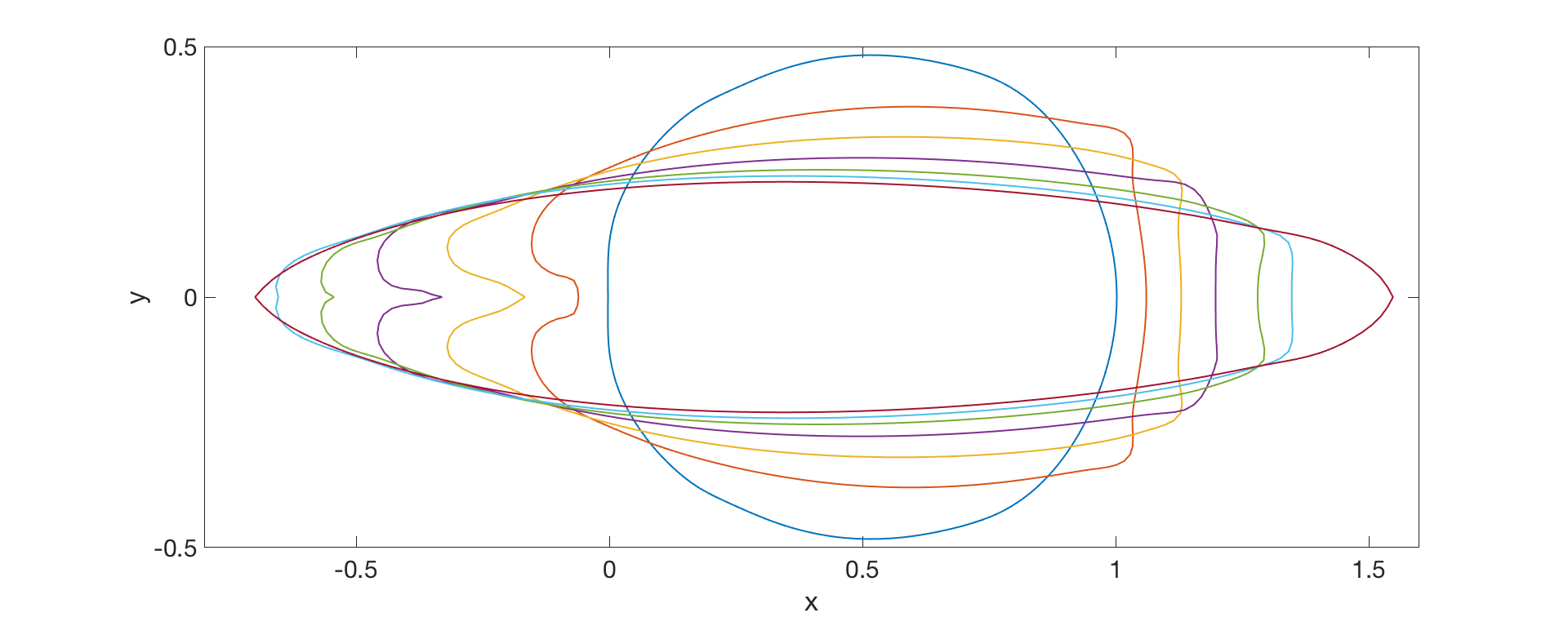
In the following, the results of the optimization when using common preconditioner (30) will be presented and compared to the common choice of Sobolev smoothing (33) with a constant smoothing parameter ϵ~\tilde{\epsilon}, which we call global preconditioning. A good smoothing parameter for the global method, has been determined by investigating the grid resolution as done in [11]. As discussed, the local methods picks the smoothing parameter automatically by minimizing (32). The task is to minimize the drag of a two dimensional cylinder, which is placed inside a fluid. To prevent the methods from simply decreasing the volume of the cylinder in order to achieve a minimization of the drag, we employ a volume constraint, which ensures a constant obstacle volume. The radius of the cylinder is one meter. We use a farfield density of 998.2​k​gm3998.2\frac{kg}{m^{3}} and a farfield velocity of 10−5​ms10^{-5}\frac{m}{s} for the Reynolds number of 11 and a velocity of 6.4⋅10−5​ms6.4\cdot 10^{-5}\frac{m}{s} for the Reynolds number of 8080. The chosen viscosity is 0.798⋅10−3​N​sm20.798\cdot 10^{-3}\frac{Ns}{m^{2}}.

6.1 Flow case 1: Re = 1

We first look at the flow with R​e=1Re=1, where we are confident to use the analytic form of β2\beta_{2} and especially β1\beta_{1}. The regularization parameter η\eta in (26) is set to 0.20.2. As commonly done in Newton’s method, we use a step length of 1.01.0 for the local method. When comparing the first design update of the local and the global method when using a step length of 11, one observes that the global method is penalized as the design update is much smaller. This is why we scale the step size of the global method, such that the magnitude of the design change will be of the same size for both methods in the first design step, see Figure 12(b). Let us now compare the optimization histories of local and global preconditioning. In Figure 12(a), we can see that using the analytic derivation of the scaling parameters β\beta as well as the information on the local frequencies inside the gradient will lead to a speedup, compared to the common global preconditioner. Whereas global preconditioning needs 1515 iterations to decrease the drag by roughly six percent, the local method will reach this reduction after nine iterations. A comparison of the flow field before and after the optimization can be found in Figure 13.

Refer to caption
(a) Optimization history
Refer to caption
(b) Scaled search direction iteration 11.
Figure 12: Comparison of standard and local preconditioning for R​e=1Re=1.
Refer to caption
Refer to caption
Figure 13: Zoomed view of the flow solution. Top: Original design and velocity magnitude. Bottom: Locally optimized design and velocity magnitude.

6.2 Flow case 2: Re = 80

We now turn to the more complicated convective case, where we choose a Reynolds number of 8080. Again, we modify the surface of a cylinder in order to reduce the drag. Remembering the numerical investigation of the Hessian matrix for such a flow, it is obvious, that we cannot use the analytic values of β1\beta_{1} as scaling parameter, whereas the values of β2\beta_{2} fit the analytic prediction. A reasonable choice for β1\beta_{1} is a scaled and smoothed version of β2\beta_{2}, which can be seen when looking at the numeric results of Figure 9. Therefore, we choose β1=10​β2\beta_{1}=10\beta_{2}, where the scaling of 1010 is motivated by the value β1F​D\beta_{1}^{FD}, which we calculated when choosing multiple frequencies, see Figure 8(a). Furthermore, we use Sobolev smoothing with a very small choice of the smoothing parameter ϵ≈10−4\epsilon\approx 10^{-4} to ensure a smooth scaling parameter β1\beta_{1}. The regularization parameter η\eta is chosen as in the first flow case, meaning that a value of 0.20.2 is taken. Due to the fact that we wish to use a constant step length for the optimization process, we use a step length of 0.50.5 for the local preconditioner and scale the search direction proposed by the global preconditioner such that both search directions are of the same size in the first optimization step. A comparison of the scaled search directions can be found in Figure 14(b).

Refer to caption
(a) Optimization history
Refer to caption
(b) Scaled search direction iteration 11.
Figure 14: Comparison of standard and local preconditioning for R​e=80Re=80.
Refer to caption
Refer to caption
Figure 15: Zoomed view of the flow solution. Top: Original design and velocity magnitude. Bottom: Locally optimized design and velocity magnitude.
Refer to caption
Refer to caption
Figure 16: Obstacle designs at iteration 1,10,20,⋯,601,10,20,\cdots,60. Top: Global preconditioning. Bottom: Local preconditioning.

During the optimization process, we see that the local preconditioner will focus on creating an optimal front and rear, whereas the global preconditioner will heavily modify the top and bottom of the obstacle. Let us now compare the optimization histories of the local and the global preconditioner, which can be seen in Figure 14(a). We see that both methods are able to heavily decrease the drag by more than 3333 percent. While the local preconditioner will reach this reduction after 6262 iterations, the global preconditioner needs 240240 iterations to reach the same drag value. It is important to note that the local preconditioner will not further decrease the drag value after iteration 6262, since the step size is too big. A smaller step size will further decrease the drag value, however we wish to perform our optimization with a constant step length, which is why subsequent drag values do not appear in the optimization history. The global method is stopped after iteration 240240 as the norm of the gradient will fall to almost zero. Let us now take a closer look at the optimized design, which can be found in Figure 15. We can see that the optimization process will create a sharp front and rear, as well as a smooth top and bottom. Comparing the design histories of the global and local method in Figure 16, we can see that the local preconditioner will focus on creating an optimal front and rear, whereas the global preconditioner will heavily modify the top and bottom of the obstacle. Note that the local method results in an inverted front, in the first design steps. However, the ability to choose non-smooth deformations is advantageous in this problem as a sharp edge is allowed to form. A disadvantage of non-smooth deformations is that it can lead to complex meshes, which is why robust mesh deformation tools need to be employed.

7 Summary and Outlook

In this paper, we derived a local smoothing preconditioner, which automatically picks smoothing parameters such that the symbol of the inverse Hessian is approximated. This preconditioner has been derived by determining the analytic symbol when choosing the Stokes equations as flow constraints. The resulting coefficients of the symbol β1\beta_{1} and β2\beta_{2}, which we called scaling parameters, have been compared to the numerical Hessian response. The presented technique to determine the scaling parameters numerically showed good agreements with the analytic results for flows with a Reynolds number of one. As convective forces become dominant, the parameter β1\beta_{1} looses validity, however β2\beta_{2} coincides with the analytic calculation. Standard Hessian manipulations of approximate Newton method have been used to obtain a sufficiently positive definite preconditioner. A computationally cheap preconditioner, which mimics the symbol of the Hessian, has been constructed by using differential operators. The derived method can be interpreted as Sobolev smoothing, which automatically picks a local smoothing parameter such that the symbol of the Hessian is approximated. Comparing the new method with Sobolev smoothing, we see that we obtain a faster convergence to the optimal design. By making use of a local smoothing parameter, which depends on the position of the optimization patch Γo\Gamma_{o}, the method is able to turn off smoothing in physically meaningful areas such as the front and rear of the cylinder.

A question that one could focus on in future work is how to determine the scaling parameter β1\beta_{1} in the case of a convective flow. Setting β1\beta_{1} to a smoothed version of β2\beta_{2} led to an acceleration of the optimization, however this choice was based on problem dependent numerical investigations, which might not hold for further applications. Furthermore, one needs to check the validity of the Hessian symbol at non-smooth parts of the optimization patch, as the symbol has been derived for smooth geometries. A construction of further preconditioners making use of the derived Hessian symbol is possible. Here, one should look at the construction of a preconditioner with pseudo-differential properties to further improve the search direction.

References

  • [1] A. Jameson, Aerodynamic design via control theory, Journal of scientific computing 3 (3) (1988) 233–260.
  • [2] A. Jameson, Automatic design of transonic airfoils to reduce the shock induced pressure drag, in: Proceedings of the 31st Israel annual conference on aviation and aeronautics, Tel Aviv, 1990, pp. 5–17.
  • [3] A. Jameson, Optimum aerodynamic design via boundary control, Vol. 94, NASA Ames Research Center, Research Institute for Advanced Computer Science, 1994.
  • [4] R. Renka, A simple explanation of the sobolev gradient method, Unpublished, University of North Texas.
  • [5] S. Kim, K. Hosseini, K. Leoviriyakit, A. Jameson, Enhancement of adjoint design methods via optimization of adjoint parameters, AIAA paper 448.
  • [6] S. J. Wright, J. Nocedal, Numerical optimization, Springer Science 35 (67-68) (1999) 7.
  • [7] E. Arian, Analysis of the Hessian for aeroelastic optimization., Tech. rep., DTIC Document (1995).
  • [8] E. Arian, S. Ta’asan, Analysis of the Hessian for aerodynamic optimization: Inviscid flow, Computers & Fluids 28 (7) (1999) 853–877.
  • [9] E. Arian, V. N. Vatsa, A preconditioning method for shape optimization governed by the Euler equations, International Journal of Computational Fluid Dynamics 12 (1) (1999) 17–27.
  • [10] S. Yang, G. Stadler, R. Moser, O. Ghattas, A shape hessian-based boundary roughness analysis of navier–stokes flow, SIAM Journal on Applied Mathematics 71 (1) (2011) 333–355.
  • [11] S. Schmidt, V. Schulz, Impulse response approximations of discrete shape Hessians with application in CFD, SIAM Journal on Control and Optimization 48 (4) (2009) 2562–2580.
  • [12] J. Sokolowski, J.-P. Zolésio, Introduction to Shape Optimization: Shape Sensitivity Analysis, Springer Berlin Heidelberg, 1992.
  • [13] M. C. Delfour, J.-P. Zolésio, Shapes and Geometries: Metrics, Analysis, Differential Calculus, and Optimization, 2nd Edition, Advances in Design and Control 22, SIAM Philadelphia, 2011.
  • [14] S. Schmidt, Efficient Large Scale Aerodynamic Design Based on Shape Calculus, Ph.D. thesis, Universität Trier (2010).
  • [15] S. Ta’asan, Trends in aerodynamics design and optimization: A mathematical viewpoint, in: Proceedings of the 12th AIAA Computational Fluid Dynamics Conference [4], 1995, pp. 961–970.
  • [16] F. Palacios, M. R. Colonno, A. C. Aranake, A. Campos, S. R. Copeland, T. D. Economon, A. K. Lonkar, T. W. Lukaczyk, T. W. Taylor, J. J. Alonso, Stanford university unstructured (su2): An open-source integrated computational environment for multi-physics simulation and design, AIAA Paper 287 (2013) 2013.
  • [17] S. Mallat, A wavelet tour of signal processing, Academic press, 1999.