Dividend and Capital Injection Optimization with Transaction Cost for Spectrally Negative Lévy Risk Processes

This paper aims to discuss the optimal impulse dividend and capital injection (IDCI) strategy for an insurance company. The surplus level is modelled by a spectrally negative Lévy (SNL) risk process, a widely used model in the literature. To enhance the practical relevance of the optimal dividend problem considered in this paper, we consider two real-life factors: the transaction costs on dividends and the capital injections. First, having the transaction costs included in the total cost of dividends is a natural addition; and second, allowing capital injections can protect the insurance company against the bankruptcy, thereby sustaining dividend payments in the long run. Through maximizing the expected accumulated discounted net dividend payments subtracted by the accumulated discounted cost of injecting capital under the proposed surplus process, we obtain the optimal IDCI strategy, which provides a useful reference for insurance companies when designing their long-term profit-sharing strategies.

The optimal dividend payout strategies have remained an active research field in the actuarial science literature for almost 60 years. Two survey papers, [1] and [2], provide thorough and insightful reviews on the classical contributions and recent progress in the field. The earliest paper in the field, [3], proved that with the option to pay out dividends from its surplus to the beneficiary until the discrete time of ruin, an insurance company should adopt a barrier dividend strategy to maximize the expected total amount of discounted dividends until ruin. However, when dividends are imposed with fixed transaction costs, recent research findings in the literature suggest that the dividend optimization problem becomes an impulse (dividend) control problem and the optimal dividend strategy is an optimal impulse dividend (OID) strategy.

Research on OID strategies has attracted much attention for a decade and has progressed well under various surplus processes. In the classical Cramér-Lundberg (CL) risk model, [4] studied an OID problem with transaction cost and tax on dividends as well as exponentially distributed claims. The obtained OID strategy reduces the reserve to level $u_{1}\in[0,u_{2})$ whenever it is above or equal to level $u_{2}$, also called a $(u_{1},u_{2})$ strategy. In the dual classical CL risk model, [5] also considered an OID problem with fixed/proportional transaction cost on dividends and derived the OID strategy via a quasi-variational inequality argument. [6] studied the OID problem with transaction costs on dividends for a class of general diffusion risk processes and derived the $(u_{1},u_{2})$ OID strategy. In the context of SNL risk process, [7] discussed an OID problem with transaction cost and showed that a $(u_{1},u_{2})$ strategy maximizes the expected accumulated present value of the net dividends. For the spectrally positive Lévy (SPL) risk process with fixed transaction costs on dividends, [8] proved that a $(u_{1},u_{2})$ strategy is again the OID. For more results on impulse dividend control problems, we refer readers to [9]-[15] and the references therein.

In the literature, capital injection is another factor to consider when designing dividend payout. Under risk models with dividends as well as fixed transaction costs imposed on the capital injections, the corresponding optimization problem is also an impulse (capital injection) control problem. In the setting of the dual classical CL risk model, [15] found that the optimal dividend and capital injection (ODCI) strategy, which maximizes the expected present value of the dividends subtracted by the discounted cost of capital injections, pays out dividends according to a barrier strategy and injects capitals to bring the reserve up to a critical level whenever it falls below $0$. Under the drifted diffusion risk model, [16] investigated the optimal dividend problem of an insurance company which controls risk exposure by reinsurance and by issuing new equity to protect the insurance company from bankruptcy. The corresponding ODCI strategy also pays dividends by a barrier strategy and injects capital to bring reserve up to a critical level whenever it falls below $0$. In the setting of SPL risk process with the dividend rate restricted, [17] and [18] considered an ODCI problem and found that the optimal method of paying dividends is a threshold strategy. For more information on dividend optimization in risk models with capital injection being imposed with proportional or fixed transaction cost, we refer readers to [11], [19]-[23], and the references therein.

Regarding SNL risk processes, the majority of dividend optimization problems are formulated as non-impulse stochastic control problems. Using the expected present value of dividends until ruin (the expected present value of the dividends subtracted by the discounted costs of capital injections) as the value function, [24] identified the condition under which the barrier strategy (respectively, the barrier dividend strategy together with capital injection strategy that reflects the reserve process at $0$) is optimal among all admissible strategies. More results of non-impulse dividend optimization under the SNL risk processes can be found in [10], [25]-[34], and the references therein. The non-impulse dividends optimization under the SPL risk processes can be found in [8], [14], [17], [18], [21]-[24], [30], [35], and others.

Motivated by [7] and [24], this paper studies a general optimal IDCI problem through maximizing the expected accumulated discounted net dividend payment subtracted by the accumulated discounted cost of injecting capital in the setup of the SNL risk process. The novelty in this paper lies as follows: (i) compared with the existing OID results under diffusion or general Lévy setup, the present model brings in the capital injection in an optimal way to reflect the corresponding risk process at $0$; and (ii) compared with the existing OID results concerning capital injections, the present model studies the Lévy setup, a more general driven process. In this paper, the discussion follows the standard treatment of Hamilton-Jacobi-Bellman (HJB) inequality in the control theory. We first find the optimal strategy among all $(z_{1},z_{2})$ IDCI strategies, and then we prove that it is optimal among all IDCI strategies via a verification argument. To facilitate the standard HJB framework, we employ subtle approaches within each step, for example, the novel technique to derive Proposition 3.3 and Lemma 4.6, and the mollifying argument to prove the modified verification lemma (see, Lemma 4.3 and Lemma 4.4).

We acknowledge that there is a parallel paper in the literature, [36], which was also finished independently around the same time. The first version of both papers were available on internet in the middle of 2018. The authors of [36] considered the bail-out optimal dividend problem under fixed transaction costs for a Lévy risk model with a constraint on the expected net present value of injected capital. While the main results in this paper and those in [36] appear to be very similar, the primary objectives of these two papers are notably different as well as the methods adopted in the proof of certain main results (for instance, the verification Lemma 4.3 and Lemma 4.4 in this paper vs Theorem 4.10 in [36]). We believe both papers make interesting contributions to the literature.

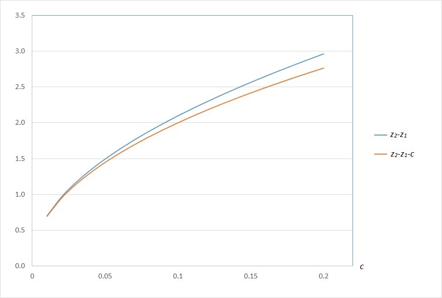
The remainder of this paper is organized as follows: Section 2 comprises preliminaries concerning the SNL process and the mathematical setup of the dividend optimization problem. In Section 3 we represent the value function of a $(z_{1},z_{2})$ IDCI strategy using the scale function associated with the SNL process. This facilitates the characterization of the optimal strategy among all $(z_{1},z_{2})$ IDCI strategies, which is further proved to be optimal among all admissible IDCI strategies. In Section 4, we first prove that a solution to the HJB inequalities coincides with the optimal value function via a verification lemma. Next, the solution to the HJB inequality is constructed, and the optimal strategy is found to be a $(z_{1},z_{2})$ IDCI strategy under which the risk process is reflected at $0$. In Section 5, we also illustrate the optimal IDCI strategy by using one numerical example.

Let $X=\{X(t);t\geq 0\}$ with probability law $\{\mathrm{P}_{x};x\in\left[0,\infty\right)\}$ and natural filtration $\mathcal{F}=\{\mathcal{F}_{t};t\geq 0\}$ be a SNL process, which is not a pure increasing linear drift or the negative of a sub-ordinator. Denote the running supremum $\overline{X}(t):=\sup\{X(s);s\in[0,t]\}$ for $t\geq 0$. Assume that in the case of no control (dividend is not deducted and capital is not injected), the risk process evolves as $X(t)$ for $t\geq 0$. An impulse dividend strategy, denoted by $D=\{D(t);t\geq 0\}$, is a one-dimensional, non-decreasing, left-continuous, $\mathcal{F}$-adapted, and pure jump process started at $0$, i.e., $D(0)=0$ and $D(t)$ defines the cumulative dividend that the company has paid out until time $t\geq 0$. For the insurance company not to go bankrupt, the beneficiary of the dividend is required to inject capital into the insurance company to ensure that the risk process is non-negative. A capital injection strategy, denoted by $R=\{R(t);t\geq 0\}$, is a one-dimensional, non-decreasing, càdlàg, $\mathcal{F}$-adapted process started at $0$, i.e., $R(0)=0$ and $R(t)$ defines the cumulative capital that the beneficiary has injected until time $t\geq 0$. The combined pair $(D,R)$ is called an IDCI strategy. More explicitly, an impulse dividend strategy $D$ is characterized by

where $\tau_{n}^{D}$ and $\eta_{n}^{D}$ are the $n$-th time and amount of dividend lump sum payment, respectively. With dividends deducted according to $D$ and capital injected according to $R$, the controlled aggregate reserve process is then given by

An IDCI strategy $(D,R)$ is defined to be admissible if $U(t)\geq 0$ for all $t\geq 0$ and $\int_{0}^{\infty}\mathrm{e}^{-qt}\mathrm{d}R(t)<\infty$ almost sure in the sense of $\mathrm{P}_{x}$, where $q>0$ is a discount factor.

Let $\mathcal{D}$ be the set of all admissible dividend and capital injection strategies. For an IDCI strategy $(D,R)\in\mathcal{D}$, denote its value function as

where $c>0$ is the transaction cost for each lump sum dividend payment and $\phi>1$ is the cost of per unit capital injected. The goal is to identify the optimal strategy $(D^{*},R^{*})$ and the corresponding optimal value function

Intuitively speaking, because of $\phi>0$ and $q>0$, it would be better if the capital is injected as late as possible with no further capital injection being made rather than just injecting enough amounts to keep the corresponding risk process non-negative.

The Laplace exponent of $X$ is

where $\upsilon$ is the Lévy measure with $\int_{(0,\infty)}(1\wedge x^{2})\upsilon(\mathrm{d}x)<\infty$. Alternatively,

where $B(t)$ is the standard Brownian motion, $N(\mathrm{d}s,\mathrm{d}x)$ is an independent Poisson random measure on $[0,\infty)\times(0,\infty)$ with intensity measure $\mathrm{d}s\upsilon(\mathrm{d}x)$, and $\overline{N}(\mathrm{d}s,\mathrm{d}x)=N(\mathrm{d}s,\mathrm{d}x)-\mathrm{d}s\upsilon(\mathrm{d}x)$ denotes the compensated random measure.

It is known that $\psi(\theta)<\infty$ for $\theta\in[0,\infty)$, in which case it is strictly convex and infinitely differentiable. As in [37], the $q$-scale function of $X$, for each $q\geq 0$, $W^{(q)}:[0,\infty)\mapsto[0,\infty)$ is the unique strictly increasing and continuous function with Laplace transform

where $\Phi_{q}$ is the largest solution of the equation $\psi(\theta)=q$. Further, let $W^{(q)}(x)=0$ for $x<0$ and write $W$ for the $0$-scale function $W^{(0)}$. For any $x\in\mathbb{R}$ and $\vartheta\geq 0$, there exists the well-known exponential change of measure for an SNL process

Furthermore, under the probability measure $\mathrm{P}_{x}^{\vartheta}$, $X$ remains an SNL process and we denote by $W_{\vartheta}^{(q)}$ and $W_{\vartheta}$ respectively the $q$-scale function and the $0$-scale function for $X$ under $\mathrm{P}_{x}^{\vartheta}$.

Note that we do not impose the safety loading condition $\psi^{\prime}(0+)\geq 0$. Instead, $\psi^{\prime}(0+)>-\infty$ is assumed throughout the paper.

For the Lévy process $X$, denote the reflected process at infimum (or at $0$)

Define $T_{a}^{+}=\inf\{t\geq 0;Y(t)>a\}$ and $\tau_{a}^{+}=\inf\{t\geq 0;U(t)>a\}$, respectively, to be the up-crossing times of level $a\geq x$ of the processes $Y$ and $U$, with the convention $\inf\emptyset=\infty$. Define further

Then, for $x\in[0,b]$ and $q\geq 0$, Proposition 2 of [38] holds that

For $z_{1}<z_{2}$, let us consider an important type of IDCI strategy, such as the $(z_{1},z_{2})$ strategy $\{(D_{z_{1}}^{z_{2}}(t),R_{z_{1}}^{z_{2}}(t));t\geq 0\}$: a lump sum of dividend payment is made to bring the reserve level down to the level $z_{1}$ once the reserve hits or is above the level $z_{2}$, while no dividend payment is made whenever the reserve level is below $z_{2}$. Capital is injected in such a way that the reserve process is reflected at $0$ , i.e., $R_{z_{1}}^{z_{2}}(t)=-\inf\limits_{0\leq s\leq t}\left(X(s)-D_{z_{1}}^{z_{2}}(s)\right)\wedge 0$. To be precise, we define recursively $T_{0}^{+}=0,\,\,T_{1}^{+}=T_{z_{2}}^{+}$ and

Then, the $(z_{1},z_{2})$ strategy can be re-expressed as

and

In the following result, the value function of a $(z_{1},z_{2})$ strategy, denoted by $V_{z_{1}}^{z_{2}}$, is expressed in terms of the scale functions.

Define, for $0<c\leq z_{1}+c<z_{2}<\infty$,

Then, $V_{z_{1}}^{z_{2}}(x)=Z^{(q)}(x)\xi(z_{1},z_{2})+\phi\left(\overline{Z}^{(q)}(x)+\frac{\psi^{\prime}(0+)}{q}\right),\,\,x\in[0,z_{2}]$. The set of maximizers of $\xi(z_{1},z_{2})$ is written as

Denote by

the first passage time of the Lévy process reflected at its supremum. The following result gives a useful link between the second derivative of $\xi$ (in $z_{2}$) and the Laplace transform of $\hat{\tau}_{z_{2}}$.

The following result characterizes the optimal IDCI strategy among all $(z_{1},z_{2})$ strategies.

References

• (1) Albrecher, H., Thonhauser, S.: Optimality results for dividend problems in insurance. Rev. R. Acad. Cien. Serie A. Mat. 103(2), 295-320 (2009).
• (2) Avanzi, B.: Strategies for dividend distribution: A review. N. Am. Actuar. J. 13(2), 217-251 (2009).
• (3) De Finetti, B.: Su un’impostazion alternativa dell teoria collecttiva del rischio. In Trans. XVth Internat. Congress Actuaries 2, 433-443 (1957).
• (4) Bai, L., Guo, J.: Optimal dividend payments in the classical risk model when payments are subject to both transaction costs and taxes. Scand. Actuar. J. 2010(1), 36-55 (2010).
• (5) Zhou, M., Yiu, K.: Optimal dividend strategy with transaction costs for an upward jump model. Quant. Financ. 14(6), 1097-1106 (2014).
• (6) Bai, L., Paulsen, J.: Optimal dividend policies with transaction costs for a class of diffusion processes, SIAM J. Control Optim. 48, 4987-5008 (2010).
• (7) Loeffen, R.: An optimal dividends problem with transaction costs for spectrally negative Lévy processes. Insur. Math. Econ. 45, 41-48 (2009).
• (8) Bayraktar, E., Kyprianou, A., Yamazaki, K.: Optimal dividends in the dual model under transaction costs. Insur. Math. Econ. 54, 133-143 (2014).
• (9) Hernández, C., Junca, M., Moreno-Franco, H.: A time of ruin constrained optimal dividend problem for spectrally one-sided Lévy processes. Insur. Math. Econ. 79, 57-68 (2018).
• (10) Avram, F., Palmowski, Z., Pistorius, M.: On Gerber-Shiu functions and optimal dividend distribution for a Lévy risk process in the presence of a penalty function. Ann. Appl. Probab. 25(4), 1868-1935 (2015).
• (11) Zhao, Y., Wang, R., Yao, D., Chen, P.: Optimal dividends and capital injections in the dual model with a random time horizon. J. Optimiz. Theory App. 167, 272-295 (2015).
• (12) Guan, H., Liang, Z.: Viscosity solution and impulse control of the diffusion model with reinsurance and fixed transaction costs. Insur. Math. Econ. 54, 109-122 (2014).
• (13) Hunting, M., Paulsen, J.: Optimal dividend policies with transaction costs for a class of jump-diffusion processes. Financ. Stoch. 17(1), 73-106 (2013).
• (14) Avanzi, B., Shen, J., Wong, B.: Optimal dividends and capital injections in the dual model with diffusion. ASTIN Bull. 41(2), 611-644 (2011).
• (15) Yao, D., Yang, H., Wang, R.: Optimal dividend and capital injection problem in the dual model with proportional and fixed transaction costs. Eur. J. Oper. Res. 211(3), 568-576 (2011).
• (16) Peng, X., Chen, M., Guo, J.: Optimal dividend and equity issuance problem with proportional and fixed transaction costs. Insur. Math. Econ. 51(3), 576-585 (2012).
• (17) Zhao, Y., Wang, R., Yin, C.: Optimal dividends and capital injections for a spectrally positive Lévy process. J. Ind. Manag. Optim. 12(4), 1-21 (2017).
• (18) Zhao, Y., Chen, P., Yang, H.: Optimal periodic dividend and capital injection problem for spectrally positive Lévy processes. Insur. Math. Econ. 74, 135-146 (2017).
• (19) Zhu, J.: Optimal financing and dividend distribution with transaction costs in the case of restricted dividend rates. ASTIN Bull. 47(1), 239-268 (2017).
• (20) Avram, F., Pérez, J., Yamazaki, K.: Spectrally negative Lévy processes with Parisian reflection below and classical reflection above. Stoch. Proc. Appl. 128(1), 255-290 (2018).
• (21) Avanzi, B., Pérez, J., Wong, B., Yamazaki, K.: On optimal joint reflective and refractive dividend strategies in spectrally positive Lévy models. Insur. Math. Econ. 72, 148-162 (2017).
• (22) Yin, C., Yuen, K.: Optimal dividend problems for a jump-diffusion model with capital injections and proportional transaction costs. J. Ind. Manag. Optim. 11(4), 1247-1262 (2015).
• (23) Bayraktar, E., Kyprianou, A.E., Yamazaki, K.: On optimal dividends in the dual model. ASTIN Bull. 43(3), 359-372 (2013).
• (24) Avram, F., Palmowski, Z., Pistorius, M.: On the optimal dividend problem for a spectrally negative Lévy process. Ann. Appl. Probab. 17, 156-180 (2007).
• (25) Loeffen, R.: On optimality of the barrier strategy in de Finetti’s dividend problem for spectrally negative Lévy processes. Ann. Appl. Probab. 18, 1669-1680 (2008).
• (26) Loeffen, R.: An optimal dividends problem with a terminal value for spectrally negative Lévy processes with a completely monotone jump density. J. Appl. Probab. 46(1), 85-98 (2009).
• (27) Loeffen, R., Renaud J.: De Finetti’s optimal dividends problem with an affine penalty function at ruin. Insur. Math. Econ. 46(1), 98-108 (2010).
• (28) Kyprianou, A., Palmowski, Z.: Distributional study of de Finetti’s dividend problem for a general Lévy insurance risk process. J. Appl. Probab. 44(2), 428-443 (2007).
• (29) Renaud, J., Zhou, X.: Distribution of the present value of dividend payments in a Lévy risk model. J. Appl. Probab. 44, 420-427 (2007).
• (30) Kyprianou, A., Loeffen, R., Pérez, J.: Optimal control with absolutely continuous strategies for spectrally negative Lévy processes. J. Appl. Probab. 49(1), 150-166 (2012).
• (31) Boguslavskaya, E.: Optimization problems in financial mathematics: Explicit solutions for diffusion models. Doctoral Thesis, University of Amsterdam (2008).
• (32) Thonhauser, S., Albrecher, H.: Dividend maximization under consideration of the time value of ruin. Insur. Math. Econ. 41, 163-184 (2007).
• (33) Azcue, P., Muler, N.: Optimal reinsurance and dividend distribution policies in the Cramér Lundberg model. Math. Financ. 15, 261-308 (2005).
• (34) Gerber, H.: Entscheidungskriterien fur den zusammengesetzten Poisson-Prozess. Mit. Verein. Schweiz. Versicherungsmath. 69, 185-227 (1969).
• (35) Yin, C., Wen, Y.: Optimal dividend problem with a terminal value for spectrally positive Lévy processes. Insur. Math. Econ. 53(3), 769-773 (2013).
• (36) Junca, M., Moreno-Franco, H., Pérez, J.: Optimal bail-out dividend problem with transaction cost and capital injection constraint. Risks 7(1), 13 (2019).
• (37) Bertoin, J.: Lévy Processes. Cambridge University Press, Cambridge (1996).
• (38) Pistorius, M.: On exit and ergodicity of the spectrally one-sided Lévy process reflected at its infimum. J. Theor. Probab. 17(1), 183-220 (2004).
• (39) Kyprianou, A.: Introductory Lectures on Fluctuations of Lévy Processes with Applications. Springer, Berlin (2006).
• (40) Wang, W., Zhou, X.: General draw-down based de Finetti optimization for spectrally negative Lévy risk processes. J. Appl. Probab. 55(2), 513¨C542 (2018).
• (41) Asmussen,S.: Ruin Probabilities. World Scientific Publishing, Singapore (2000).
• (42) Hubalek, F., Kyprianou, A.: Old and new examples of scale functions for spectrally negative Lévy processes. In Sixth Seminar on Stochastic Analysis, Random Fields and Applications (R. Dalang, M. Dozzi and F. Russo, Eds.) 119-145. Springer, Basel (2011).
• (43) Jacod, J., Shiryaev, A.: Limit Theorems for Stochastic Processes (Second edition). Springer-Verlag, Berlin, Heidelberg (2003).
• (44) Ikeda, N., Watanabe, S.: Stochastic Differential Equations and Diffusion Processes. North Holland-Kodansha, New York (1981).
• (45) Protter, P.: Stochastic Integration and Differential Equations. Springer, Berlin (1995).
• (46) Højgaard, B., Taksar, M.: Controlling risk exposure and dividends payout schemes: Insurance company example. Math. Financ. 9(2), 153-182 (1999).