Residual Balancing: A Method of Constructing Weights for Marginal Structural ModelsThanks: Direct all correspondence to Xiang Zhou, Department of Government, Harvard University, 1737 Cambridge Street, Cambridge, MA 02138, USA; email: xiang_zhou@fas.harvard.edu. The authors benefited from communications with Justin Esarey, Kosuke Imai, Gary King, José Zubizarreta, and participants of the Applied Statistics Workshop at Harvard University, the Political Methodology Speaker Series at MIT, and the 35th Annual Meeting of the Society for Political Methodology at Brigham Young University.
Abstract
When making causal inferences, post-treatment confounders complicate analyses of time-varying treatment effects. Conditioning on these variables naively to estimate marginal effects may inappropriately block causal pathways and may induce spurious associations between treatment and the outcome, leading to bias. To avoid such bias, researchers often use marginal structural models (MSMs) with inverse probability weighting (IPW). However, IPW requires models for the conditional distributions of treatment and is highly sensitive to their misspecification. Moreover, IPW is relatively inefficient, susceptible to finite-sample bias, and difficult to use with continuous treatments. We introduce an alternative method of constructing weights for MSMs, which we call “residual balancing.” In contrast to IPW, it requires modeling the conditional means of the post-treatment confounders rather than the conditional distributions of treatment, and it is therefore easier to use with continuous exposures. Numeric simulations suggest that residual balancing is both more efficient and more robust to model misspecification than IPW and its variants. We illustrate the method by estimating (a) the cumulative effect of negative advertising on election outcomes and (b) the controlled direct effect of shared democracy on public support for war. Open source software is available for implementing the proposed method.
1 Introduction
Social scientists are often interested in estimating the marginal, or population average, effects of treatment in the presence of post-treatment confounding. Post-treatment confounding is common in studies of time-varying treatments, where confounders of future treatments may be affected by prior treatments. For example, political scientists study how the timing and frequency of negative advertising during political campaigns affect election outcomes (e.g., Lau, Sigelman and Rovner 2007; Blackwell 2013). In this context, the decision to run negative advertisements at any given point during a campaign is affected by a candidate’s position in recent polling data, which itself is affected by negative advertising conducted previously. Post-treatment confounding is also common in analyses of causal mediation, where confounders for the effect of the mediator on the outcome may be affected by treatment. For example, when assessing the role of morality in mediating the effects of shared democracy on public support for war, post-treatment variables, such as beliefs about the threat posed by the adversary, may affect both the perceived morality of war and support for military action (Tomz and Weeks 2013).
Conventional methods that adjust for post-treatment confounders by conditioning, stratifying, or matching on them naively may engender two different types of bias (Robins 1986; Robins 1999). First, adjusting naively for post-treatment confounders leads to bias from over-control of intermediate pathways because it blocks, or “controls away,” the effect of treatment on the outcome that operates through these variables. Second, adjusting naively for post-treatment confounders can lead to collider-stratification bias if these variables are also affected by unobserved determinants of the outcome, as conditioning on a variable generates a spurious association between its common causes even when these common causes are unconditionally independent (Pearl 2009).
To avoid these biases, researchers typically use marginal structural models (MSMs) and the associated method of inverse probability weighting (IPW), which yields consistent estimators of treatment effects under fairly general conditions (Robins 1999; Robins, Hernan and Brumback 2000; VanderWeele 2015). Nevertheless, IPW is not without limitations. First, IPW requires models for the conditional distributions of exposure to treatment and/or the mediator, and prior research indicates that it is highly sensitive to their misspecification (Mortimer et al. 2005; Kang and Schafer 2007; Lefebvre, Delaney and Platt 2008; Howe et al. 2011). Second, even if these models are correctly specified, IPW is relatively inefficient, and it is susceptible to large finite-sample biases when confounders strongly predict the exposures of interest (Wang et al. 2006; Cole and Hernán 2008).11 1 For expositional simplicity, we occasionally use the term “exposures” to generally refer to treatments or mediators. Finally, when the exposures of interest are continuous, IPW tends to perform poorly because estimates of conditional densities are often unreliable (e.g., Vansteelandt 2009; Naimi et al. 2014).
Several remedies have been proposed to improve the efficiency and robustness of IPW. For example, Cole and Hernán (2008) suggest truncating or censoring extreme weights to obtain more precise estimates. With this method, however, the improved precision comes at the cost of greater bias. Recently, Imai and Ratkovic (2014); Imai and Ratkovic (2015) propose constructing weights for an MSM with covariate balancing propensity scores (CBPS). By integrating a large set of balancing conditions when estimating propensity scores, this method is less sensitive to model misspecification. But estimating CBPS can be computationally demanding, and because of the practical difficulties associated with modeling conditional densities, this method is not well suited for continuous exposures (see Fong et al. 2018 and Yiu and Su 2018 for extensions of CBPS to continuous exposures in the cross-sectional setting).
In this paper, we propose an alternative method of constructing weights for MSMs, which we call “residual balancing.” Briefly, the method is implemented in two stages. First, a model for the conditional mean of each post-treatment confounder, given past treatments and confounders, is estimated and then used to construct residual terms. Second, a set of weights is constructed using Hainmueller’s (2012) entropy balancing method such that, in the weighted sample, (a) the residualized confounders are orthogonal to future exposures, past treatments, and past confounders, and (b) their discrepancy with a set of base weights (e.g., survey sampling weights) is minimized. Thus, our proposed method is an extension of Hainmueller’s (2012) entropy balancing procedure to the longitudinal setting. It exactly balances sample moments for each of the post-treatment confounders across future exposures, conditional on the observed past, without explicit models for the conditional distributions of exposure to treatment and/or a mediator.
This method has a number of advantages over IPW and its variants. First, residual balancing is relatively robust to the model misspecification bias that commonly afflicts these other methods. Second, residual balancing is also more efficient because it tends to avoid highly variable and extreme weights by minimizing their relative entropy with respect to a set of base weights. Third, because it does not require models for the conditional distributions of the exposures, residual balancing is easy to use with continuous treatments and/or mediators. Finally, in contrast to CBPS, residual balancing is computationally attractive in that the weighting solution is quickly obtained even with a large number of confounders, time periods, and observations. An open source R package, rbw, is available for implementing the proposed method.
In the sections that follow, we first briefly review MSMs and the method of IPW. Next, we introduce the method of residual balancing, and conduct a set of simulation studies to evaluate its performance relative to IPW and its variants. We then illustrate the method empirically by estimating the cumulative effect of negative advertising on election outcomes as well as the controlled direct effect (CDE) of shared democracy on public support for war. We conclude by discussing the method’s limitations along with possible remedies.
2 MSMs and IPW: A Review
In this section, we briefly review MSMs and the method of IPW (Robins 1999; Robins, Hernan and Brumback 2000). Consider first a study with time points where interest is in the effect of a time-varying treatment, (), on an end-of-study outcome, . At each time point, there is also a vector of observed time-varying confounders, , that may be affected by prior treatments. Following convention, we use overbars to denote the treatment history, , and confounder history, , up to time . Similarly, we denote an individual’s complete treatment and confounder histories through the end of follow-up by and , respectively. Finally, we use to denote the potential outcome under the particular treatment history .
An MSM is a model for the marginal mean of the potential outcomes, which can be expressed in general form as follows:
| (1) |
where is some function of treatment history, , and a parameter vector, , that captures the marginal effects of interest. For example, with a large number of time points and a binary treatment, a common parameterization is
| (2) |
where denotes the total number of time periods on treatment and captures the marginal effect of one additional wave on treatment. Of course, many other parameterizations are possible.
An MSM can be identified from observed data under three key assumptions:
- 1.
consistency, which requires that, for any unit, if , then ;
- 2.
sequential ignorability, which requires that treatment at each time point must not be confounded by unobserved factors conditional on past treatments and observed confounders, or formally, that for any treatment sequence ; and
- 3.
positivity, which requires that treatment assignment must not be deterministic, or formally, that for any treatment condition if , where denotes a probability mass or density function.
When these assumptions are satisfied, an MSM can be consistently estimated using the method of IPW.
IPW estimation involves fitting a model for the conditional mean of the observed outcome given an individual’s treatment history using weights that balance, in expectation, past confounders across treatment at each time point. The inverse probability weight for individual is defined as
| (3) |
where the term can be ignored when . Since the denominator of equation (3) can be very small, some units may end up with extremely large weights, leading to highly variable estimates. To mitigate this problem, Robins, Hernan and Brumback (2000) suggest using a so-called “stabilized” weight, which is defined as
| (4) |
Sometimes, the probabilities in both the numerator and denominator are also made conditional on a set of baseline or time-invariant confounders :
| (5) |
In such cases, these variables need to be included in the MSM to properly adjust for confounding, which is unproblematic because they cannot be affected by treatment.
In practice, both the numerator and the denominator of the stabilized weight need to be estimated. When treatment is binary, the denominator is typically estimated using a generalized linear model (GLM), with the logit or probit link function, for treatment at each time point, while the numerator is estimated using a constrained version of this model that omits the time-varying confounders. When treatment is continuous, models are needed to estimate the conditional densities in both the numerator and the denominator of the weight. After weights have been computed, the marginal effects of interest are estimated by fitting a model for the conditional mean of given with weights equal to . When both this model and the models for treatment assignment are correctly specified, this procedure yields consistent estimates for all marginal means of the potential outcomes, , and thus for any marginal effect of interest, provided that the identification assumptions outlined previously are satisfied.
As shown in prior studies (e.g., Lefebvre, Delaney and Platt 2008; Howe et al. 2011), IPW estimates of marginal effects can be highly sensitive to misspecification of the models used to construct the weights. To address this limitation, Imai and Ratkovic (2014); Imai and Ratkovic (2015) developed the method of CBPS to estimate the denominator in equation (4) for binary treatments. With a logit model for treatment at each time point, this method augments the score conditions of the likelihood function with a set of covariate balance conditions. Because the number of balance conditions may exceed the number of model parameters to be estimated, the generalized method of moments (GMM) is used to minimize imbalance in the weighted sample. This method of incorporating balance conditions into model-based estimation of the weights tends to reduce the bias that results when the treatment models are misspecified (see Tan 2017 for a theoretical discussion on the robustness of calibrated propensity scores).
MSMs and IPW estimation can also be used to examine causal mediation (VanderWeele 2015). Consider now a study with a point-in-time treatment, , a putative mediator measured at some point following treatment, , and an end-of-study outcome, . Suppose that both treatment and the mediator are confounded by a vector of observed pre-treatment covariates, denoted by , and that the mediator is additionally confounded by a vector of observed post-treatment covariates, denoted by , which may be affected by the treatment received earlier. In this setting, the potential outcomes of interest are denoted by .
As before, an MSM models the marginal mean of the potential outcomes. If, for example, treatment and the mediator are both binary, a saturated MSM can be expressed as follows:
| (6) |
From this model, the controlled direct effect of treatment is given by , which measures the strength of the causal relationship between treatment and the outcome when the mediator is fixed at a given value, , for all individuals (Pearl 2001; Robins 2003). This estimand is useful for assessing causal mediation because it helps to adjudicate between alternative explanations for a treatment effect. For example, the difference between a total effect and the may be interpreted as the degree to which the mediator contributes to a causal mechanism that transmits the effect of treatment on the outcome (Acharya, Blackwell and Sen 2016; Zhou and Wodtke 2019).
MSMs for the joint effects of a treatment and mediator, like equation (6), can be identified under essentially the same assumptions as outlined previously. In this context, the consistency assumption requires that if and ; sequential ignorability requires that both treatment and the mediator must be unconfounded conditional on the observed past, or formally, that and ; and positivity requires that both treatment and the mediator are not deterministic functions of past variables. Similarly, the stabilized inverse probability weights are here defined as
| (7) |
and they must be estimated using appropriate models for the conditional probabilities and/or densities that compose this expression. After weights have been computed, the marginal effects of interest – here, the – are estimated by fitting a model for the conditional mean of given and with weights equal to . Alternatively, it is also possible to define the weights as , in which case must be included in the MSM to properly adjust for confounding. Adjusting for in the MSM is unproblematic because these variables are not post-treatment confounders, unlike .
3 Residual Balancing
In this section, we motivate and explain the method of residual balancing. We first focus on analyses of time-varying treatment effects, and then we outline how the method is easily adapted for studies of causal mediation. Finally, we discuss similarities and differences between residual balancing and the CBPS method proposed by Imai and Ratkovic (2015).
3.1 Rationale
To explain the method of residual balancing, it is useful to begin with Robins’ (1986) g-computation formula. The g-computation formula factorizes the marginal mean of the potential outcome, , as follows:
| (8) |
In contrast, the conditional mean of the observed outcome given can be factorized into
| (9) |
A comparison of equation (8) with equation (9) indicates that weighting the observed population by
| (10) |
would yield a pseudo-population in which and thus , where the asterisk denotes quantities in the weighted pseudo-population.22 2 In fact, the “stabilized” weight in equation (4) is just a different way of writing equation (10): Because is often high-dimensional, estimation of the conditional densities in equation (10) is practically difficult.
Nevertheless, the condition that implies that, in the pseudo-population, the following moment condition would hold for any scalar function of :
| (11) |
This moment condition can be equivalently expressed as
| (12) |
where is a residual transformation of with respect to its conditional mean given the observed past. The moment condition in equation (12) in turn implies that for any scalar function of and , and are uncorrelated, that is,
| (13) |
where the second equality follows from the fact that .
The method of residual balancing emulates the moment conditions (13) that would hold in the pseudo-population were it possible to weight by . In other words, it emulates the moment conditions (13) that would be expected in a sequentially randomized experiment. Specifically, this is accomplished by (a) specifying a set of functions, , and a set of functions, ; (b) computing a set of residual terms, , from the observed data; and then (c) finding a set of weights such that, for any , , and , the cross-moment of and is zero in the weighted data. Hence, it involves finding a set of nonnegative weights, denoted by , subject to the following balancing conditions:
| (14) |
or, expressed more succinctly,
| (15) |
where is the th element of and is the total number of balancing conditions. The conditions in equation (14) stipulate that the residualized confounders at each time point are balanced across future treatments, past treatments, and past confounders, or some function thereof. In this way, the proposed method adjusts for post-treatment confounding without engendering bias due to over-control or collider-stratification, as the residualized confounders are balanced across future treatments while (appropriately) remaining orthogonal to the observed past.
As long as the convex hull of contains , finding the weighting solution is an under-identified (or just-identified) problem. Following Hainmueller (2012), we minimize the relative entropy between and a set of base weights (e.g., a vector of ones or survey sampling weights),33 3 Alternative loss functions, such as the empirical likelihood (Fong et al. 2018) or the variance (Zubizarreta 2015), could also be used to construct the weights. We use the relatively entropy metric because it can easily accommodate a set of base weights. Moreover, in contrast to the empirical likelihood, the relatively entropy metric is convex and thus computationally convenient.
| (16) |
subject to the balancing conditions. This is a constrained optimization problem that can be solved using Lagrange multipliers. Technical details can be found in Supplementary Material A (see also Hainmueller 2012).
3.2 Implementation
In practice, residual balancing requires specifying a set of functions that constitute . A natural choice is to set , where is the th element of the covariate vector . If there is concern about confounding by higher-order or interaction terms, they can also be included in . Then, the residual terms, , need to be estimated from the data. Because , they can be estimated by fitting GLMs for and then extracting the response residuals, , where is a vector of regressors and denotes the inverse link function of the GLM.
In addition, residual balancing requires specifying a set of functions that constitute . Because weighting is intended to neutralize the relationship between and future treatments, we suggest including all future treatments, , ,, in . However, if it is reasonable to assume that the effects of on future treatments stop at , where , treatments beyond time may be excluded from . Equation (13) additionally indicates that should be uncorrelated with past treatments, , and past confounders, , in the weighted pseudo-population. Because by construction, zero correlation is guaranteed in the original unweighted population, and when the GLMs for are Gaussian, binomial, or Poisson regressions with canonical links, the score equations ensure that the response residuals, , are orthogonal to the regressors in the original sample. But to ensure that the response residuals, , are also orthogonal to the regressors in the reweighted sample, we suggest including all members of in .
In general, then, should include all future treatments as well as all regressors in the GLMs for , including an intercept. A reassuring property of this specification for is that if the GLMs for are Gaussian, binomial, or Poisson regressions with canonical links and they are fit to the weighted sample with all future treatments, , as additional regressors, the coefficients on future treatments will all be exactly zero and the coefficients on will be the same as those in the original sample. Therefore, when the GLMs for are correctly specified, the first moments of are guaranteed to be balanced across future treatments, conditional on past treatments and confounders, as would be expected in a scenario where treatment is unconfounded by .
In sum, a typical implementation of residual balancing for estimating the marginal effects of a time-varying treatment proceeds in two steps:
- 1.
At each time point and for each confounder , fit a linear, logistic, or Poisson regression of , as appropriate given its level of measurement, on and , and then compute the response residuals, .
- 2.
Find a set of weights, , such that:
- (a)
in the weighted sample, the residuals, , are orthogonal to all future treatments and the regressors of ; and
- (b)
the relative entropy between and the base weights, , is minimized.
- (a)
The weighting solution can then be used to fit any MSM of interest.
3.3 Application to Causal Mediation
Residual balancing can also be used to estimate an MSM for the joint effects of a point-in-time treatment, , and mediator, , in the presence of both pre-treatment confounders, , and a set of post-treatment confounders, , for the mediator-outcome relationship. In this setting, residual balancing is implemented using essentially the same procedure as outlined previously but with several minor adaptions. First, for each pre-treatment confounder , compute the response residuals, , by centering it around its sample mean. Then, for each post-treatment confounder , fit a linear, logistic, or Poisson regression of , depending on its level of measurement, on and , and then compute the response residuals, . Finally, find a set of weights, , such that, in the weighted sample, the pre-treatment residuals are orthogonal to both treatment and the mediator , the post-treatment residuals are orthogonal to treatment, the mediator, and the pre-treatment confounders ; and the relative entropy between and the base weights is minimized. The weighting solution can then be used to fit any MSM for the joint effects of the treatment and mediator on the outcome, from which the controlled direct effects of interest are constructed. Alternatively, it is also possible to skip the first step and construct weights that only balance the residualized post-treatment confounders, in which case the pre-treatment confounders must be included as regressors in the MSM.
3.4 Comparison with IPW and CBPS
Compared with IPW, residual balancing has several advantages. First, because it does not require explicit models for the conditional probability/density of exposure to treatment and/or a mediator, residual balancing is robust to the bias that results when these models are misspecified, and it is easy to use with both binary and continuous exposures. Second, by minimizing the relative entropy between the balancing weights and the base weights, the method tends to avoid highly variable and extreme weights, thus yielding more efficient estimates of causal effects.
Residual balancing is similar to the CBPS method (Imai and Ratkovic 2015) in that it seeks a set of weights that balance time-varying confounders across future treatments by explicitly specifying a set of balancing conditions. Residual balancing differs from CBPS, however, in two important respects. First, unlike CBPS, residual balancing can easily accommodate continuous treatments and/or mediators. As mentioned previously, this is because residual balancing does not require parametric models for exposure to treatment and/or a mediator, and thus it can balance confounders across both binary and continuous treatments using a common set of balancing conditions (equation 14). CBPS, by contrast, is based on a parametric model for the propensity score, and it is therefore limited to settings with binary treatments and/or mediators.
Second, residual balancing allows for the specification of more flexible and parsimonious balancing conditions than those specified with the CBPS method. In fact, CBPS can be viewed as an extreme form of residual balancing. To see the connection, note that CBPS attempts to balance the time-varying confounders across all possible sequences of future treatments within each possible history of past treatments. Thus, for each confounder , there are balancing conditions at time . Summing over and , the total number of balancing conditions associated with CBPS is . Because , it can easily exceed the sample size, in which case the balancing conditions are at best approximated. With residual balancing, the number of balancing conditions depends on the choice of and . As mentioned previously, a natural choice of is . If is then modeled with a saturated GLM of on only, and is defined as a set of dummy variables for each possible sequence of future treatments interacted with each possible history of past treatments, the balancing conditions in equation (14) would be equivalent to those for the CBPS method.
With residual balancing, however, , , and can be specified more flexibly. For example, when a parsimonious GLM is used for , and only the regressors of and future treatments are included in , the number of balancing conditions will be , which is substantially smaller than . In large and even moderately size samples, these balancing conditions can often be satisfied exactly.
4 Simulation Experiments
In this section, we conduct a set of simulation studies to assess the performance of residual balancing for estimating marginal effects with (a) a binary time-varying treatment under correct model specification, (b) a continuous time-varying treatment under correct model specification, (c) a binary time-varying treatment under incorrect model specification, and (d) a continuous time-varying treatment under incorrect model specification. In each of these four settings, we compare residual balancing with four variants of IPW: conventional IPW with weights estimated from GLMs (IPW-GLM), IPW with weights estimated from GLMs and then censored (IPW-GLM-Censored), IPW with weights estimated from CBPS (IPW-CBPS), and as a benchmark, IPW with weights based on the true exposure probabilities (IPW-Truth). Because the CBPS method has not been extended for continuous treatments in the time-varying setting, we assess the performance of IPW-CBPS only for binary treatments.
The data generating process (DGP) in our simulations is very similar to that of Imai and Ratkovic (2015). It involves four time-varying covariates measured at time periods with a sample of . At each time , the covariates are determined by treatment at time and a multiplicative error: , where , for and for . Treatment at each time depends on prior treatment at time and the covariates . Specifically, when treatment is binary, it is generated as a Bernoulli draw with probability , and when treatment is continuous, it is generated as , where and . Here, we use the parameter to control the level of treatment-outcome confounding. We consider two values of , 0.4 and 0.8, corresponding to scenarios where treatment-outcome confounding is mild and strong, respectively. Finally, the outcome is generated as , where . To assess the impact of model misspecification, we use the same DGP, but we recode the “observed” covariates as nonlinear transformations of the “true” covariates: specifically, . We then use only the transformed covariates, , to implement IPW, its variants, and residual balancing. Note that the conditional mean model for is still correct when the treatment is binary but incorrect when the treatment is continuous.
For each scenario described previously, we generate 2,500 random samples. Then, for each sample, we construct weights using IPW-GLM, IPW-GLM-Censored, IPW-CBPS, and residual balancing. With IPW-GLM, we estimate the weights using logistic regression for binary treatments and normal linear models for continuous treatments, assuming homoskedastic errors. With IPW-GLM-Censored, we follow Cole and Hernán’s (2008) example and censor weights at the 1st and 99th percentiles. With IPW-CBPS, we estimate weights using the methods proposed by Imai and Ratkovic (2015) with the function CBMSM() in the R package CBPS. With residual balancing, , and the residual terms are estimated from linear models for with prior treatment as a regressor, and includes as well as the regressors in the model for (i.e., 1 and ). Finally, with each set of weights, we fit an MSM by regressing the outcome on the three treatment variables and denote their coefficient estimates as , , and . We obtain the true values of these coefficients by simulating potential outcomes with the g-computation formula, regressing them on the treatment variables, and averaging their coefficients over a large number of simulations. The performance of each method is evaluated using the simulated sampling distributions of , , and .
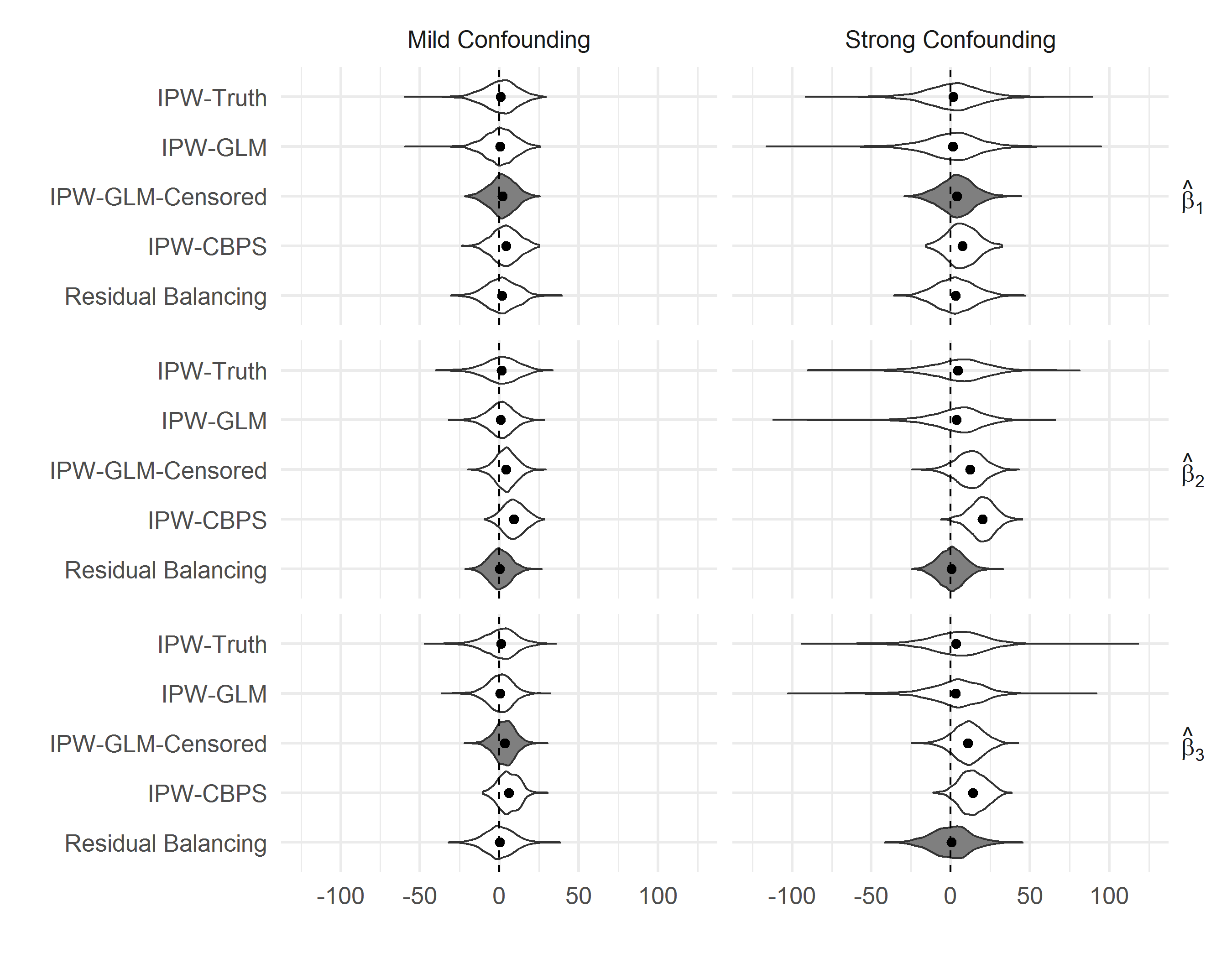

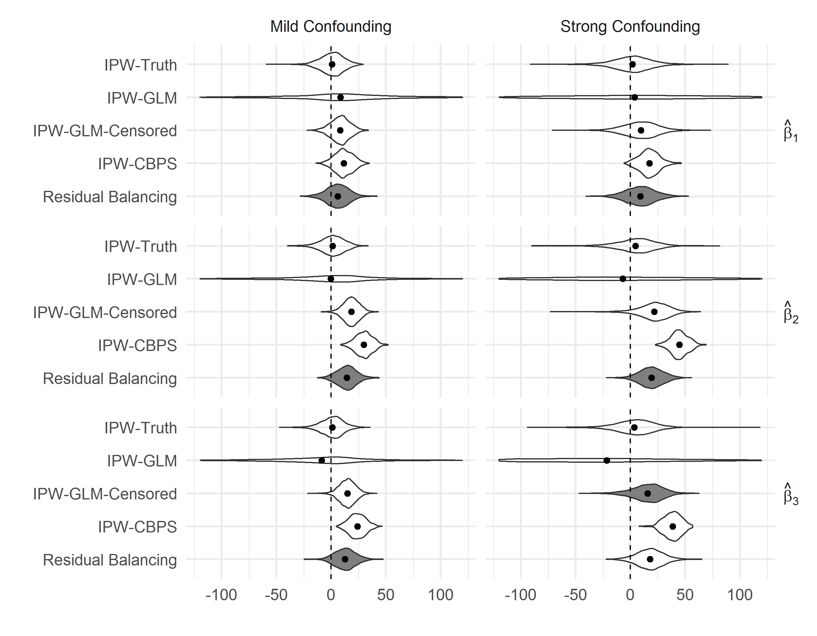

Figure 1 presents results from simulations with a binary treatment and correct model specification. Specifically, this figure displays a set of violin plots, which show the sampling distributions of , , and centered at the true values of these coefficients. In these plots, black dots represent means of the sampling distributions, and the shaded distributions highlight the estimator with the smallest root mean squared error (RMSE) in each scenario.
Two patterns are evident from Figure 1. First, comparing the left and right panels, we see that IPW and its variants suffer from finite-sample bias and may have skewed sampling distributions, especially when the covariates are strongly predictive of treatment. By contrast, residual balancing is roughly unbiased, and its estimates appear approximately normally distributed, regardless of the level of confounding. Second, the results in Figure 1 indicate that residual balancing is much more efficient than IPW-GLM, especially when the level of confounding is high. In addition, with a high level of confounding, both IPW-GLM-Censored and IPW-CBPS yield much less variable estimates than IPW-GLM, but this gain in precision comes at the expense of greater bias. Residual balancing, by contrast, improves efficiency without inducing bias.
Figure 2 presents another set of violin plots based on simulations with a continuous treatment and correct model specification. As before, the bias for IPW and its variants increases substantially with the level of confounding. Residual balancing, by contrast, is approximately unbiased across all levels of confounding. Moreover, residual balancing consistently outperforms IPW and its variants in terms of efficiency.44 4 Note that IPW based on true probability densities (IPW-Truth) is often not as efficient as IPW based on estimated densities (IPW-GLM), which suggests that “over-fitting” the treatment models can lead to efficiency gains when these models are correctly specified (Rubin and Thomas 1996; Hirano, Imbens and Ridder 2003). For example, residual balancing is the most accurate and precise estimator for and under both high and low levels of confounding (For , the performance of residual balancing is comparable to that of IPW-GLM-Censored). In sum, residual balancing matches or exceeds the performance of IPW and its variants across all scenarios in these simulations.
Figure 3 presents violin plots from simulations with a binary treatment and misspecified models where is measured incorrectly. As indicated by its extreme level of sampling variation, IPW-GLM is highly unstable when models for the conditional probability of treatment are misspecified. Consistent with Imai and Ratkovic (2015), IPW-CBPS appears more robust to model misspecification, as reflected in its substantially smaller sampling variation compared with IPW-GLM. At the same time, however, this improvement in precision comes at the cost of greater bias. In addition, censoring the inverse probability weights also appears to substantially improve the method’s performance in the presence of misspecification. In fact, IPW-GLM-Censored even outperforms IPW-CBPS in these simulations. Nevertheless, despite the improvements achieved by censoring the weights or using CBPS, residual balancing consistently produces the most accurate and efficient estimates across nearly all scenarios.
Figure 4 presents violin plots from simulations with a continuous treatment and incorrect measures of , in which case both the treatment assignment model for IPW and the confounder models for residual balancing are misspecified. Consistent with the results discussed previously, this figure also indicates that IPW-GLM is extremely biased and inefficient, that censoring the weights reduces bias and improves efficiency, and that residual balancing yields by far the most accurate and efficient estimator among all methods. Note that residual balancing even outperforms IPW based on the true propensity scores, despite the fact that the confounder models are now misspecified.
5 The Cumulative Effect of Negative Advertising on Vote Shares
In this section, we illustrate residual balancing empirically by estimating the cumulative effect of negative campaign advertising on election outcomes (Lau, Sigelman and Rovner 2007; Blackwell 2013; Imai and Ratkovic 2015). Drawing on U.S. senate and gubernatorial elections from 2000 to 2006, Blackwell (2013) used MSMs with IPW to evaluate the cumulative effects of negative campaign advertising on election outcomes for 114 Democratic candidates. MSMs are appropriate for this problem because campaign advertising is a dynamic process plagued by post-treatment confounding. For example, candidates adjust their campaign strategies on the basis of current polling results, where trailing candidates are more likely to “go negative” than leading candidates. At the same time, polling results change over time and are likely affected by a candidate’s previous use of negative advertising.
Treatment, , in this analysis is the proportion of campaign advertisements that are “negative” (i.e., that mention the opposing candidate) in each campaign-week. Because IPW tends to preform poorly with continuous treatments, we also consider a binary version of treatment, , for which the proportion of negative advertisements is dichotomized using a cutoff of 10%, as in Blackwell (2013). The time-varying confounders, , included in this analysis are the Democratic share in the polls and the share of undecided voters in the previous campaign-week. This analysis also uses a set of baseline confounders, , including total campaign length, election year, incumbency status, and whether the election is for the senate or governor’s office. The outcome, , is the Democratic share of the two-party vote.
Following Imai and Ratkovic (2015), we focus on the final five weeks preceding the election and estimate an MSM for the binary version of treatment with form
| (17) |
and an MSM for the continuous treatment with form
| (18) |
In these models, denotes the total number of campaign-weeks for which more than 10% of the candidate’s advertising was negative, denotes the average proportion of advertisements that were negative over the final five weeks of the campaign, is an indicator of incumbency status used to construct interaction terms that allow the effect of negative advertising to differ between incumbents and nonincumbents.55 5 In equations (17) and (18), the “main” effect of is captured in the term . Thus, the effect of an additional week with more than 10% negative advertising for nonincumbents is , and for incumbents, it is . Similarly, and correspond to the effects of a 1 percentage point increase in negative advertising for nonincumbents and incumbents, respectively. To facilitate comparison of results across the different versions of treatment, we report estimates for the effects of a 10 percentage point increase in negative advertising—that is, and .
We estimate these models with both IPW methods and residual balancing. Specifically, we first implement IPW-GLM by fitting, at each time point, a logistic regression of the dichotomized treatment on both time-varying confounders and baseline confounders, and then constructing the inverse probability weights using equation (5). Second, we implement IPW-CBPS with the same treatment assignment model using the function CBMSM() in the R package CBPS. Finally, we implement residual balancing by, first, fitting linear models for each covariate in () with lagged values of treatment and the time-varying confounders as regressors and extracting residual terms . For each covariate in , the residual term is computed as the deviation from its sample mean. Then, we find a set of minimum entropy weights such that, in the weighted sample, is balanced across treatment at time and the regressors of . Standard errors are computed using the robust (i.e., ‘‘sandwich’’) variance estimator.66 6 In Part B of the Supplementary Material, we report a set of simulation results on the performance of the robust variance estimator for IPW-GLM, IPW-GLM-Censored, IPW-CBPS, and residual balancing. We find that the robust variance estimator is consistently conservative for residual balancing. For IPW and its variants, the robust variance estimator appears to sometimes over-estimate and other times under-estimate the true sampling variance, depending on the particular scenario. R code for implementing residual balancing in this analysis is available in Part C of the Supplementary Material.
| Estimator | Dichotomized Treatment | Continuous Treatment | ||
|---|---|---|---|---|
| Nonincumbent | Incumbent | Nonincumbent | Incumbent | |
| IPW-GLM | 1.42 (0.43) | -1.73 (0.47) | 0.80 (0.28) | -1.15 (0.31) |
| IPW-CBPS | 0.78 (0.89) | -2.03 (0.41) | ||
| Residual Balancing | 0.98 (0.54) | -1.67 (0.46) | 0.49 (0.32) | -0.99 (0.36) |
Note: For the dichotomized treatment, results represent the estimated marginal effects of an additional week with more than 10% negative advertising. For the continuous treatment, results represent the estimated marginal effects of a 10 percentage point increase in the average proportion of negative advertisements across all campaign-weeks. Numbers in parentheses are robust (i.e., “sandwich”) standard errors.
Results from these analyses are presented in Table 1, where the first two columns contain IPW-GLM, IPW-CBPS, and residual balancing estimates based on the dichotomized version of treatment. For nonincumbent candidates, these results suggest that the effect of negative advertising is positive. However, both IPW-CBPS and residual balancing yield point estimates that are considerably smaller than IPW-GLM. While IPW-GLM suggests that an additional week with more than 10% negative advertising increases a candidate’s vote share by 1.42 percentage points, on average, the estimated effect is reduced to 0.78 percentage points for IPW-CBPS and 0.98 percentage points for residual balancing. For incumbent candidates, all three methods indicate that negative advertising has a substantively large negative effect on vote shares. Residual balancing, for example, suggests that an additional week with more than 10% negative advertising decreases a candidate’s vote share by 1.67 percentage points, on average.
The last two columns of Table 1 present results based on the continuous version of treatment. Because IPW-CBPS has not been developed for continuous treatments in the time-varying setting, we focus on estimates from IPW-GLM and residual balancing. Overall, these results are quite consistent with those based on the dichotomized treatment. For nonincumbents, the effect of negative advertising appears to be positive, although the estimate from residual balancing is relatively small. For incumbents, both methods suggest a sizable negative effect. According to the residual balancing estimate, a 10 percentage point increase in the proportion of negative advertising throughout the final five weeks of the campaign reduces a candidate’s vote share by about one percentage point, on average.
6 The Controlled Direct Effect of Shared Democracy on Public Support for War
In this section, we reanalyze data from Tomz and Weeks (2013) to estimate the controlled direct effect (CDE) of shared democracy on public support for war, controlling for a respondent’s perceived morality of war. With a nationally representative sample of 1,273 US adults, Tomz and Weeks (2013) conducted a survey experiment to analyze the role of public opinion in the democratic peace, that is, the empirical regularity that democracies almost never fight each other. In this experiment, they presented respondents with a situation in which a country was developing nuclear weapons and, when describing the situation, they randomly and independently varied three characteristics of the country: political regime (whether it was a democracy), alliance status (whether it had signed a military alliance with the United States), and economic ties (whether it had high levels of trade with the United States). They then asked respondents about their levels of support for a preventive military strike against the country’s nuclear facilities. The authors found that individuals are substantially less supportive of military action against democracies than against otherwise identical autocracies.
To investigate the causal mechanisms through which shared democracy reduces public support for war, Tomz and Weeks (2013) also measured each respondent’s beliefs about the threat posed by the potential adversary (threat), the cost of military intervention (cost), and the likelihood of victory (success). In addition, the authors also assessed each respondent’s moral concerns about using military force (morality). With these data, they conducted a causal mediation analysis and found that shared democracy reduces public support for war primarily by changing perceptions of the threat and morality of using military force. In this analysis, the authors examined the role of each mediator separately by assuming that they operate independently and do not influence one another. However, it is likely that one’s perception of morality is partly influenced by beliefs about the threat, cost, and likelihood of success, which also affect support for war directly.77 7 Tomz and Weeks (2013) acknowledged this possibility and, in an auxiliary analysis, they relaxed this assumption and estimated the indirect effect through morality that is not mediated by other mediators, i.e., the path-specific effect of democracymoralitysupport for war. However, because this effect excludes other pathways through morality (such as democracyperceived threatmoralitysupport for war), it does not fully capture the mediating role of morality. Thus, in the following analysis, we treat these variables as post-treatment confounders and reassess the mediating role of morality accordingly.
In this data set, the outcome, , is a measure of support for war on a five-point scale; treatment, , denotes whether the country developing nuclear weapons is presented as a democracy; the mediator, , is a dummy variable indicating whether the respondent thought it would be morally wrong to strike; the pretreatment covariates include dummy variables for each of the two other randomized treatments (alliance status and economic ties) as well as a number of demographic and attitudinal controls; and the post-treatment confounders include measures of the respondent’s beliefs about threat, cost, and likelihood of success.88 8 For detailed descriptions of the variables included in and , see Tomz and Weeks (2013, Table 5). We estimate the CDE of shared democracy, controlling for perceptions of morality, using an MSM with form
| (19) |
In this model, we control for the pretreatment covariates because, although treatment is randomly assigned, they may still confound the mediator-outcome relationship.99 9 Alternatively, these pretreatment confounders can be adjusted for using IPW or residual balancing weights. We adjust for them directly in the MSM for the sake of statistical efficiency. The controlled direct effect is given by , where measures the effect of shared democracy on support for war if none of the respondents had moral reservations about military intervention and measures the effect of shared democracy on support for war if all respondents thought it would be morally wrong to strike.
We estimate this model with both IPW-GLM and residual balancing weights. Specifically, we first implement IPW-GLM by fitting a logit model for with , , and as regressors, by fitting a second logit model for with only and as regressors, and then by using the fitted values from these models to estimate a set of weights with the following form: . Second, we implement residual balancing by fitting a linear model for each post-treatment confounder in with and as regressors, computing residual terms , and then finding a set of minimum entropy weights such that, in the weighted sample, is balanced across and the regressors of . Standard errors are computed using the robust (i.e., “sandwich”) variance estimator. R code for implementing residual balancing in this analysis is available in Part C of the Supplementary Material.
| Total Effect | IPW | Residual Balancing | |
|---|---|---|---|
| intercept | 2.39 (0.05) | 3.12 (0.05) | 2.76 (0.05) |
| shared democracy | -0.35 (0.07) | -0.20 (0.07) | -0.36 (0.08) |
| moral concerns | -1.63 (0.14) | -1.20 (0.13) | |
| shared democracy * moral concerns | -0.05 (0.16) | 0.14 (0.16) |
Note: Coefficients of pretreatment covariates are omitted. For ease of interpretation, all pretreatment covariates are centered at their means. Numbers in parentheses are robust (“sandwich”) standard errors.
As a benchmark, the first column of Table 2 presents an estimate of the total treatment effect from a regression of on and . Echoing the original study, we find that shared democracy significantly reduces public support for war—by 0.35 points on the five-point scale, or about 0.25 standard deviations. The next two columns present IPW and residual balancing estimates, respectively, for model (19). In this model, the “main effect” of shared democracy represents the estimated CDE if respondents had no moral reservations about military intervention, and the sum of this coefficient and the interaction term represents the estimated CDE if respondents did have moral reservations.
IPW and residual balancing yield somewhat different estimates of these effects. According to IPW, the estimated CDE of shared democracy is -0.20 if respondents had no moral concerns about war, and it is -0.25 if respondents thought it was morally wrong to strike. According to residual balancing, by contrast, the estimated CDE of shared democracy is -0.36 if respondents had no moral concerns about war, and it is -0.22 if respondents thought military intervention was morally wrong. Notwithstanding these differences, however, both IPW and residual balancing suggest that most of the total effect is “direct,” , transmitted through pathways other than morality.
7 Discussion and Conclusion
Post-treatment confounding arises in analyses of both time-varying treatments and causal mediation, where it complicates the use of conventional regression and matching methods for causal inference. To adjust for this type of confounding, researchers most often use MSMs along with the associated method of IPW estimation (Robins 1999; Robins, Hernan and Brumback 2000; VanderWeele 2015). IPW, however, is highly sensitive to model misspecification, relatively inefficient, susceptible to finite-sample bias, and difficult to use with continuous treatments. Several remedies for these problems have been proposed, such as censoring the weights (Cole and Hernán 2008) or constructing them with CBPS (Imai and Ratkovic 2014; 2015), but these corrections are not without their own limitations.
In this article, we proposed the method of residual balancing for constructing weights that can be used to estimate MSMs. In contrast to IPW, residual balancing does not require models for the conditional distribution of exposure to treatment and/or a mediator. Rather, it entails modeling only the conditional means of the post-treatment confounders, and because it simultaneously imposes covariate balancing and minimum entropy conditions on the weights, the method is both more efficient and more robust to model misspecification than IPW. It is also much easier to use with continuous treatments, which obviates the need for arbitrary quantile binning as is often employed in practice (e.g., Wodtke, Harding and Elwert 2011; Blackwell 2013).
Residual balancing appears to outperform IPW even when the weights are constructed with CBPS, which similarly incorporate explicit balancing conditions when estimating the conditional probabilities of exposure. The reason, we believe, is that IPW with CBPS attempts to balance the time-varying confounders across all possible sequences of future treatments within all possible histories of prior treatments, whereas residual balancing models the conditional means of the time-varying confounders and balances only their residuals across a parsimonious representation of future treatments and the observed past. As a result, the search for covariate balancing weights is often an over-identified problem with CBPS but an under-identified problem with residual balancing. Thus, although weights based on CBPS can improve covariate balance compared with weights estimated from conventional GLMs, the weights given by residual balancing can satisfy a set of balancing conditions exactly.
Despite its many advantages, residual balancing is still limited in several ways. First, it requires modeling the conditional means of the post-treatment confounders (or transformations thereof). When these models are misspecified, the moment condition in equation (11) is only partially achieved. In this case, equation (12) implies
where future treatments (i.e., , ,) may still be unconfounded in the weighted pseudo-population but the pseudo-population no longer mimics the original unweighted population. As a result, estimates of marginal effects based on residual balancing weights may not be consistent for the target population of interest. This limitation can be mitigated in practice, however, by fitting more flexible, non- or semi-parametric models for .
Second, even when models for the conditional means of the post-treatment confounders are correctly specified, residual balancing estimates of marginal effects may still be biased if the balancing conditions are insufficient. For example, if both the treatment and outcome are affected by the product of two confounders, say , but and are only included separately in the implementation of residual balancing, confounding may still be present in the weighted sample, leading to bias. This bias, however, can be mitigated by including a large set of functions in , such as along with other cross-product or higher-order terms. Alternatively, subject matter knowledge should guide the choice of functions in when available.
In sum, residual balancing provides an efficient and robust method of constructing weights for MSMs. It should therefore find wide application in analyses of time-varying treatments and causal mediation, wherever post-treatment confounding presents itself. To facilitate its implementation in practice, we have developed an open-source R package, rbw, for constructing residual balancing weights, which is available from GitHub: https://github.com/xiangzhou09/rbw. In addition, Part C of the Supplementary Material provides R code illustrating the use of rbw in our two empirical examples.
References
- Acharya, Blackwell and Sen (2016) Acharya, Avidit, Matthew Blackwell and Maya Sen. 2016. “Explaining Causal Findings Without Bias: Detecting and Assessing Direct Effects.” American Political Science Review 110(3):512–529.
- Blackwell (2013) Blackwell, Matthew. 2013. “A Framework for Dynamic Causal Inference in Political Science.” American Journal of Political Science 57(2):504–520.
- Cole and Hernán (2008) Cole, Stephen R and Miguel A Hernán. 2008. “Constructing Inverse Probability Weights for Marginal Structural Models.” American Journal of Epidemiology 168(6):656–664.
- Fong et al. (2018) Fong, Christian, Chad Hazlett, Kosuke Imai et al. 2018. “Covariate Balancing Propensity Score for a Continuous Treatment: Application to the Efficacy of Political Advertisements.” The Annals of Applied Statistics 12(1):156–177.
- Hainmueller (2012) Hainmueller, Jens. 2012. “Entropy Balancing for Causal Effects: A Multivariate Reweighting Method to Produce Balanced Samples in Observational Studies.” Political Analysis 20(1):25–46.
- Hirano, Imbens and Ridder (2003) Hirano, Keisuke, Guido W Imbens and Geert Ridder. 2003. “Efficient Estimation of Average Treatment Effects Using the Estimated Propensity Score.” Econometrica 71(4):1161–1189.
- Howe et al. (2011) Howe, Chanelle J, Stephen R Cole, Joan S Chmiel and Alvaro Muñoz. 2011. “Limitation of Inverse Probability-of-Censoring Weights in Estimating Survival in the Presence of Strong Selection Bias.” American Journal of Epidemiology 173(5):569–577.
- Imai and Ratkovic (2014) Imai, Kosuke and Marc Ratkovic. 2014. “Covariate Balancing Propensity Score.” Journal of the Royal Statistical Society: Series B (Statistical Methodology) 76(1):243–263.
- Imai and Ratkovic (2015) Imai, Kosuke and Marc Ratkovic. 2015. “Robust Estimation of Inverse Probability Weights for Marginal Structural Models.” Journal of the American Statistical Association 110(511):1013–1023.
- Kang and Schafer (2007) Kang, Joseph DY and Joseph L Schafer. 2007. “Demystifying Double Robustness: A Comparison of Alternative Strategies for Estimating a Population Mean from Incomplete Data.” Statistical Science 22(4):523–539.
- Lau, Sigelman and Rovner (2007) Lau, Richard R, Lee Sigelman and Ivy Brown Rovner. 2007. “The Effects of Negative Political Campaigns: A Meta-Analytic Reassessment.” Journal of Politics 69(4):1176–1209.
- Lefebvre, Delaney and Platt (2008) Lefebvre, Genevieve, Joseph AC Delaney and Robert W Platt. 2008. “Impact of Mis-specification of the Treatment Model on Estimates from a Marginal Structural Model.” Statistics in medicine 27(18):3629–3642.
- Mortimer et al. (2005) Mortimer, Kathleen M, Romain Neugebauer, Mark Van Der Laan and Ira B Tager. 2005. “An Application of Model-Fitting Procedures for Marginal Structural Models.” American Journal of Epidemiology 162(4):382–388.
- Naimi et al. (2014) Naimi, Ashley I, Erica EM Moodie, Nathalie Auger and Jay S Kaufman. 2014. “Constructing Inverse Probability Weights for Continuous Exposures: a Comparison of Methods.” Epidemiology 25(2):292–299.
- Pearl (2001) Pearl, Judea. 2001. Direct and Indirect Effects. In Proceedings of the Seventeenth Conference on Uncertainty in Artificial Intelligence. Morgan Kaufmann Publishers Inc. pp. 411–420.
- Pearl (2009) Pearl, Judea. 2009. Causality (2nd Edition). Cambrdige University Press.
- Robins (1986) Robins, James. 1986. “A New Approach to Causal Inference in Mortality Studies with a Sustained Exposure Period-Application to Control of the Healthy Worker Survivor Effect.” Mathematical Modelling 7(9-12):1393–1512.
- Robins (1999) Robins, James M. 1999. “Marginal Structural Models versus Structural Nested Models as Tools for Causal Inference.” Statistical Models in Epidemiology: The Environment and Clinical Trials .
- Robins (2003) Robins, James M. 2003. “Semantics of Causal DAG models and the Identification of Direct and Indirect effects.” Highly Structured Stochastic Systems pp. 70–81.
- Robins, Hernan and Brumback (2000) Robins, James M, Miguel Angel Hernan and Babette Brumback. 2000. “Marginal Structural Models and Causal Inference in Epidemiology.” Epidemiology 11(5):550–560.
- Rubin and Thomas (1996) Rubin, Donald B and Neal Thomas. 1996. “Matching Using Estimated Propensity Scores: Relating Theory to Practice.” Biometrics pp. 249–264.
- Tan (2017) Tan, Zhiqiang. 2017. “Regularized Calibrated Estimation of Propensity Scores with Model Misspecification and High-dimensional data.” arXiv preprint arXiv:1710.08074 .
- Tomz and Weeks (2013) Tomz, Michael R and Jessica L Weeks. 2013. “Public Opinion and the Democratic Peace.” American Political Science Review 107:849–865.
- VanderWeele (2015) VanderWeele, Tyler. 2015. Explanation in Causal Inference: Methods for Mediation and Interaction. Oxford University Press.
- Vansteelandt (2009) Vansteelandt, Stijn. 2009. “Estimating Direct Effects in Cohort and Case–control Studies.” Epidemiology 20(6):851–860.
- Wang et al. (2006) Wang, Yue, Maya L Petersen, David Bangsberg and Mark J van der Laan. 2006. “Diagnosing Bias in the Inverse Probability of Treatment Weighted Estimator Resulting from Violation of Experimental Treatment Assignment.”.
- Wodtke, Harding and Elwert (2011) Wodtke, Geoffrey T, David J Harding and Felix Elwert. 2011. “Neighborhood Effects in Temporal Perspective: The impact of Long-term Exposure to Concentrated Disadvantage on High School Graduation.” American Sociological Review 76(5):713–736.
- Yiu and Su (2018) Yiu, Sean and Li Su. 2018. “Covariate Association Eliminating Weights: A Unified Weighting Framework for Causal Effect Estimation.” Biometrika .
- Zhou and Wodtke (2019) Zhou, Xiang and Geoffrey T. Wodtke. 2019. “A Regression-with-Residuals Method for Estimating Controlled Direct Effects.” Political Analysis .
- Zubizarreta (2015) Zubizarreta, José R. 2015. “Stable Weights that Balance Covariates for Estimation with Incomplete Outcome Data.” Journal of the American Statistical Association 110(511):910–922.