Renormalon-free definition of the gluon condensate within the large- approximation
Abstract
We propose a clear definition of the gluon condensate within the large- approximation as an attempt toward a systematic argument on the gluon condensate. We define the gluon condensate such that it is free from a renormalon uncertainty, consistent with the renormalization scale independence of each term of the operator product expansion (OPE), and an identical object irrespective of observables. The renormalon uncertainty of , which renders the gluon condensate ambiguous, is separated from a perturbative calculation by using a recently suggested analytic formulation. The renormalon uncertainty is absorbed into the gluon condensate in the OPE, which makes the gluon condensate free from the renormalon uncertainty. As a result, we can define the OPE in a renormalon-free way. Based on this renormalon-free OPE formula, we discuss numerical extraction of the gluon condensate using the lattice data of the energy density operator defined by the Yang–Mills gradient flow.
PTEP-subject
B01, B06, B32, B651 Introduction
In perturbative expansion of observables in quantum chromodynamics (QCD), the coefficients of the series typically grow factorially as a function of the order and thus the perturbation series is an asymptotic series at best [1]. One of the origins of this growth is the factorial increase in the number of Feynman diagrams with respect to the order. In the renormalized perturbation theory, there is another origin: there exists a class of Feynman diagrams whose amplitude grows factorially [2, 1, 3]. This kind of factorial behavior produces the so-called renormalon ambiguity in perturbation theory of order , where is the one-loop coefficient of the beta function, the renormalized coupling, constant and parametrizes the “strength” of the renormalon; is the renormalization group invariant mass scale and is a typical energy scale in the problem under consideration. ( in our convention.) Particularly for the (dimensionless) observables which are Lorentz invariant and dependent on a single energy scale, perturbative calculations suffer from the so-called renormalon, and have the inevitable uncertainty of . Examples of such observables are the Adler function, the plaquette, the energy density operator defined by the Yang--Mills gradient flow, etc.11 1 The static QCD potential at very short distances also suffers from the renormalon, although it is not Lorentz invariant.
The operator product expansion (OPE), which is an extended framework of perturbation theory, is considered to be helpful in overcoming the error due to the renormalon. The OPE of a general observable with the above properties is of the form
| (1.1) |
in quenched QCD. Here, the coefficients and denote the Wilson coefficients, and the symbol stands for renormalization. (We can adopt, for instance, the scheme to define renormalized composite operators.) The Wilson coefficients are calculated in perturbation theory, whereas the vacuum expectation values (VEVs) of composite operators are generally nonperturbative objects. In particular, the VEV of is known as the gluon condensate. (These condensates are zero in perturbative calculations in dimensional regularization.) Hence, the Wilson coefficient is given by perturbative calculation of and possesses the renormalon uncertainty of . This error is the same order of magnitude as the second term of the OPE, the first nonperturbative effect specified by the gluon condensate. Hence, the gluon condensate has been considered as a key element to overcome the error due to the renormalon. In particular, since the gluon condensate appears universally in the OPE and conceptually has a unique value irrespective of observables, determining this value (in some way) would be quite helpful; it allows us to predict terms of many observables.
However, in order to determine the gluon condensate numerically in the context of the OPE, one cannot avoid the issue of how to deal with the renormalon uncertainty in . In fact, the gluon condensate cannot be determined in the following naive treatment. From the OPE (1.1), the gluon condensate is read off from the coefficient of the term in while measuring an observable nonperturbatively (for instance using lattice). However, since has an error of , the determined gluon condensate has an error of , which is the same size as the gluon condensate itself. We note that the renormalon uncertainty is the minimum error of perturbation theory. Thus, this argument indicates that the gluon condensate has a significant error even when one has sufficiently large-order results.
There have been some proposals concerning treatment of to extract the gluon condensate [6, 4, 7, 5, 8] (see also Ref. [9]). An often adopted prescription is to use that is obtained by truncating the perturbative series at the th order where the th order term is minimal among the terms in the perturbative series. However, the following properties are not assured in this prescription: (i) each term in the OPE is independent of the renormalization scale, and (ii) the gluon condensate is a universal and identical object irrespective of observables. Regarding the first issue, the truncation order varies depending on the renormalization scale since it is given by . It is explicitly shown in Ref. [10] that, in the so-called large- approximation, a different choice of renormalization scale indeed changes the truncated result of . This indicates that is dependent on the renormalization scale and so is the second term, which contradicts the property usually used that each term of the OPE is independent of the renormalization scale.22 2 An appropriate redefinition of the renormalized operator and can make each of them renormalization scale independent at all order since the operator is proportional to the trace part of the energy–momentum tensor, which is renormalization scale independent. This issue is not relevant to the present argument because the problem is whether the combination of , which is independent of the redefinition, is renormalization scale dependent or not. We also note that the renormalized operator is renormalization scale independent at the one-loop level. In addition to this, the gluon condensate defined in this way has not been shown to be identical to the ones defined from other observables. If property (ii) is not assured, an extracted value of the gluon condensate from an observable has a very limited meaning: it cannot be used as an input in the OPE (1.1) of other observables.
In this paper, using the large- approximation [11, 12, 13], we propose a definition of the gluon condensate which explicitly satisfies (i) and (ii). That is, our definition of the gluon condensate is compatible with the renormalization scale independence of each term of the OPE and is unique irrespective of observables. Thus, it qualifies as an input to the term of the OPE of broad observables. Also, it does not suffer from the renormalon uncertainty of .
We achieve this as follows. We regularize the all-order perturbative series of by introducing an infrared (IR) cutoff scale . Following Refs. [10, 14], we separate this regularized Wilson coefficient into its cutoff-dependent and -independent parts, which correspond to the renormalon uncertainty and renormalon-independent (renormalon-free) parts, respectively. The renormalon-free part becomes the first term in our OPE. On the other hand, the renormalon uncertainty of 33 3 This renormalon uncertainty corresponds to the renormalon uncertainty, which one encounters in a regularization without using the IR cutoff. is absorbed into the second term of the OPE. It will be shown for some explicit observables that the renormalon uncertainty of the gluon condensate (which is exhibited as the ultraviolet (UV) cutoff dependence) is exactly canceled by this procedure. In other words, each term of our OPE (up to the second term) can be defined as a renormalon-free object. In particular, the second term of our OPE is specified by the renormalon-free gluon condensate whose definition is explicitly given in this paper. In this construction, each term of the OPE is also independent of the renormalization scale (that is different from the cutoff scale). This is realized because the first term of our OPE (the renormalon-free part of ) is obtained based on the all-order perturbative series, which is renormalization scale independent. Moreover, the gluon condensate defined in this paper is observable independent, which is related to the universality of the renormalon cancelation.
We note that in deriving these features, the large- approximation is always assumed. At this stage, it is not obvious how the relations and formulas presented in this paper are modified beyond this approximation. Also, since the large- approximation is accurate only at the leading logarithmic level, it is difficult to obtain some physical consequences, such as the value of the defined gluon condensate, from comparison of our theoretical result with the lattice result. (To determine the gluon condensate precisely, we at least have to know the large-order perturbative behavior as already mentioned.)
Nevertheless, we believe that the present work makes an improvement in our conceptual understanding of the gluon condensate because we can explicitly show how the gluon condensate is made well defined. It is also notable that the large- approximation can simulate well the divergent behavior of perturbative series caused by renormalons. We thus expect that the present work provides a foundation to define a gluon condensate with good nature [(i) and (ii)] in a more systematic approach beyond this approximation.
The paper is organized as follows. In Sect. 2, we give a definition of the renormalon-free gluon condensate, which is based on the renormalon cancelation in the OPE. In this section, we treat general observables with the renormalon as the first IR renormalon. In Sect. 3, we study some examples and confirm the renormalon cancelation explicitly. A main example is the energy density operator defined by the Yang–Mills gradient flow. The conclusions and discussion are given in Sect. 4. In Appendix A, we collect our notational conventions. In Appendix B, we explain construction of the large- approximation in the context of the gradient flow. In Appendix C, we compare the perturbative series of the energy density operator defined by the Yang–Mills gradient flow obtained in the exact calculations and in the large- approximation. In Appendix D, we report an attempt at a numerical determination of the gluon condensate, applying the formula presented in this paper.
2 Renormalon-free definition of the gluon condensate
To define the gluon condensate unambiguously in the OPE, it is necessary to separate the associated renormalon uncertainty from the Wilson coefficient in Eq. (1.1). For this, we use the formulation proposed in Ref. [10], a review of which is given in Sect. 2.1. In Sect. 2.2, we present a definition of the renormalon-free gluon condensate in light of the renormalon cancelation, and in Sect. 2.3, we consider the scheme dependence of a renormalon-free gluon condensate.
2.1 Formula to separate the renormalon in
We consider a Euclidean dimensionless observable which depends on a single scale and has the first IR renormalon at . Let us assume that the leading-order (LO) term of in perturbation theory is and is given by a one-gluon exchanging diagram. This is the case, for instance, for the Adler function44 4 We study the reduced Adler function, where term is subtracted. and the energy density operator defined by the Yang–Mills gradient flow. For such observables, we can construct all-order perturbative series in the so-called large- approximation [11, 12, 13].
The construction is as follows (see also Appendix B). We consider insertion of a chain of fermion bubbles into the gluon propagator of the LO diagram; see Fig. 1. Each bubble produces a factor proportional to , where is the number of flavors, a renormalization scale, and the gluon momentum. In Appendix A, we present our convention for the normalization factors. In the large- approximation, we replace , where55 5 We define the beta function as , where .
| (2.1) |
and then obtain the series as
| (2.2) |
The function is the integrand determined from the LO diagram. In the first equality, we use the fact that the perturbative series of coincides with that of in the context of the OPE. This is because the condensates in Eq. (1.1) are nonperturbative objects and zero in perturbative evaluation (with dimensional regularization). We note that before the replacement the series gives the leading contribution in the large- limit. However, the large- approximation obtained after this replacement is not justified in any limit of the QCD parameters. Nevertheless, this series gives the exact leading-logarithmic (LL) contribution of perturbative series. In addition, it is empirically known that this series gives a good approximation of the first few to several terms which have been calculated explicitly.

The series in the large- approximation can be resummed and expressed as
| (2.3) |
where is the modulus of the gluon momentum ; is a dimensionless function originating from 66 6 An explicit relation between and is given by where . and depends on a single variable ; and is the running coupling specific in the large- approximation,
| (2.4) |
Here, we used the expression of the one-loop running coupling , where is a renormalization group independent scale: . We note that Eq. (2.3) is independent of the renormalization scale.
Equation (2.3) is just formal because the integrand has a single pole on the integration path at . We regularize this quantity with an IR cutoff scale :
| (2.5) |
where . This resummed quantity explicitly depends on the regularization parameter (the cutoff scale). This feature that the resummation depends on how to be regularized is common in the presence of IR renormalons. In this formulation, the IR renormalons are related to the function : the IR renormalons determine the expansion of in [15]. In particular, the renormalon as the first IR renormalon leads to
| (2.6) |
where is an (-independent) constant. Thus, the cutoff dependence (dependence on ) of Eq. (2.5) is determined by the IR renormalons. In this sense, the cutoff dependence corresponds to the renormalon uncertainty. On the other hand, a cutoff-independent part, which potentially exists, corresponds to the renormalon-free part.
This motivates us to extract the cutoff-independent part from Eq. (2.5), which is precisely calculated in a renormalon-free way. This is carried out by (I) rewriting the integrand by a new analytic function defined in the complex -plane and satisfying for , and then (II) deforming the integration contour in the complex plane. The function can be constructed by
| (2.7) |
With this function we can rewrite Eq. (2.5) as
| (2.8) |
where the integration contours and are displayed in Fig. 2.


The integral along is obviously independent of . Actually, we also obtain -independent parts from the integral along . In this integral, we first expand in :
| (2.9) |
As a generic feature with the first IR renormalon at , the coefficients of the and terms are real whereas the coefficient of the term is complex. ( is a polynomial of .) This follows from Eq. (2.6) and for . For a real part (i.e., a term with coefficient ), the integral is evaluated as
| (2.10) |
In the first equality, we used a property of the integrand . Thus, the integration path can be deformed to a circle surrounding the pole, which yields the -independent result. On the other hand, the integral of the -term,
| (2.11) |
remains dependent. In this way, we have separated the -independent part , which is the renormalon-free part, from the -dependent part:
| (2.12) |
where consists of all the -independent contributions [up to ]:
| (2.13) |
In Eq. (2.12), the first term, , is independent and its asymptotic form is [10]. The second term is dependent and represents the leading dependence of as .77 7 This inevitable uncertainty of order corresponds to the uncertainty which one encounters in the resummation using the Borel integral where the integration contour is deformed as . Thus, the first term gives a dominant contribution at large due to . Hence, Eq. (2.12) can be regarded as an expansion in . The last term of generally has both cutoff-independent and -dependent terms, but dose not play any role in the following discussion.
Applying this formulation, one can calculate for explicit observables. In particular, once the function for the observable under consideration is obtained, one can follow the above calculations. As an example, we will study the energy density operator defined by the Yang–Mills gradient flow in Sect. 3.
2.2 Renormalon-free definition of the gluon condensate in light of renormalon cancelation
Let us consider the relation between the Wilson coefficient we have calculated [] and the OPE. We have regularized the Wilson coefficient with the IR cutoff scale . This implies that UV contributions are calculated as the perturbative contribution. Accordingly, it is natural that the remaining mode below the cutoff scale is represented by the nonperturbative contributions.88 8 This is analogous to the integration-by-regions argument [16, 17], where hard contributions in loop integrals are identified with Wilson coefficients whereas soft contributions correspond to condensates. Hence, we introduce as the UV cutoff scale to the condensates in the OPE. Thus, we perform the OPE as
| (2.14) |
where the gluon condensate possesses the UV cutoff scale . For , we eliminate the argument since it is a -independent constant under the approximation we consider.99 9 As seen from the explicit calculation in Eq. (2.17) below, has the same order of magnitude as in the large- approximation. (They are .) Since in the OPE Eq. (2.14), each term has the same order of magnitude in the large- approximation, the coefficient , which is calculated in perturbation theory, is thus and does not have -dependence. (We note that is renormalization scale independent at the one-loop level.)
In Eq. (2.14), the cutoff dependence should be canceled in the sum of the first and second terms because the observable is independent of the cutoff. Remember that the cutoff dependence of the first term represents the renormalon uncertainty. Hence, such a cancelation corresponds to the renormalon cancelation in the OPE. If this is true, the dependence of the second term of Eq. (2.14) should be given by
| (2.15) |
since the cutoff dependence is canceled in the quantity
| (2.16) |
and is defined as the first integral [cf. Eq. (2.5)]. In Eq. (2.15), we used the expansion of given in Eq. (2.6). In fact, Eq. (2.15) can be reduced to the relation between the coefficients and . To see this, we calculate the gluon condensate in the large- approximation with the UV cutoff. In calculating this local product, we use a naive point-splitting regularization and then contract the gauge fields. It reads
| (2.17) |
with
| (2.18) |
This cutoff dependence is regarded as the renormalon uncertainty of the gluon condensate.1010 10 We believe that the cutoff dependence of the gluon condensate can be calculated in perturbation theory due to . On the other hand, its exact behavior (determined by the low energy dynamics) cannot be obtained in perturbation theory (as the expression based on perturbation theory [right-hand side of Eq. (2.17)] is not well-defined). One sees that, using Eq. (2.17), both sides of Eq. (2.15) have the same integral. Hence, the renormalon cancelation (2.15) requires
| (2.19) |
We confirm the relation (2.19) (equivalent to the renormalon cancelation) for explicit examples below (Sect. 3). Thus, we use this relation in the following general argument.
We now define the renormalon-free gluon condensate. Using the separation formula obtained in Eq. (2.12), we express the OPE (2.14) as
| (2.20) |
Then using the relation (2.19), we obtain
| (2.21) |
Here we make the renormalon uncertainty of absorbed into the second term and define the renormalon-free gluon condensate as
| (2.22) |
We now can perform the OPE where each term is free from the renormalon uncertainty [as shown in the last expression of Eq. (2.21)].
The features of our definition of the gluon condensate (2.22) can be stated as follows. First, it is certainly free from the renormalon (or independent of the cutoff scale) since the second term in Eq. (2.22) exhibits the opposite dependence to the first term calculated in Eq. (2.17). Secondly, the definition does not have observable dependence. In other words, the symbol does not appear in Eq. (2.22) but is encoded only in its Wilson coefficient . (We note that the operator is obviously observable independent because it is a basis of the OPE taken universally for general observables.) Thus, the gluon condensate (2.22) is a universal quantity. This is compatible with its original (and naive) concept. Note that realization of this feature is not trivial a priori in the presence of the renormalon uncertainty. Thirdly, each term of the OPE [in the last expression of Eq. (2.21)] is renormalization scale independent. This stems from the fact that the first term is renormalization scale independent (since it is based on the all-order perturbative series) and the observable is, of course, renormalization scale independent. This is again consistent with the original OPE structure. In this way, we realize the definition of a gluon condensate with the desired properties.
The renormalon-free gluon condensate is considered to have a nonperturbative contribution. Thus, it is difficult to calculate this quantity theoretically. Instead, treating it as a fitting parameter, we extract its value from comparison of the renormalon-free OPE (2.21) with a measurement of (for instance using lattice simulations)—see Appendix D.1111 11 The first term can always be calculated theoretically according to the above method. This quantity depends only on the dynamical scale and is independent of the regularization parameter . We again emphasize that the value of the gluon condensate is common regardless of the chosen observables. Hence, once its value is determined from an observable, its value can be used in the renormalon-free OPE (2.21) of other observables as an input to predict the terms. Such a prediction is beyond perturbation theory because it overcomes the error of the renormalon uncertainty of .
2.3 Conversion to other schemes
There are potentially many schemes to define the renormalon-free gluon condensate. In this sense, we adopt one of possible schemes. Scheme conversion can be done by changing the identification of a cutoff-independent part. One can change a cutoff-independent part to
| (2.23) |
where is a (-independent) constant. Then, the OPE (2.20) is rearranged in this different scheme as
| (2.24) |
where
| (2.25) |
It is notable that in order to keep the observable-independent nature of the renormalon-free gluon condensate, the parameter should be taken as , where is an arbitrary constant and is independent of observables. Namely, is not completely arbitrary but should be proportional to . Once is taken in this way, the renormalon-free gluon condensate defined in this new scheme satisfies the three features stated in Sect. 2.2. However, as seen from this discussion, it seems quite natural to choose the scheme with , where the gluon condensate is obviously independent of observables. In addition, the scheme where corresponds to a minimal subtraction of the cutoff dependence of the gluon condensate.
We note that the existence of other schemes as above is not problematic. This is because the gluon condensate is not directly related to a physical observable but is a partial contribution to it. Thus the gluon condensate can be scheme dependent in the above sense. We also note, however, that we have now clarified the relation between different schemes as given in Eq. (2.25). This allows us to compare the gluon condensates in different schemes systematically.
3 Explicit examples
In this section, we study explicit examples: the Adler function and the energy density operator defined by the Yang–Mills gradient flow.
We also mention previous work concerning the static QCD potential.
We explicitly confirm the renormalon cancelation (2.19) for these quantities.
3.1 Adler function
As the first example, we consider the reduced Adler function [18].1212 12 The reduced Adler function is defined such that its perturbative expansion starts at . It is defined as
| (3.1) |
for and , where is a correlator of the quark current ,1313 13 Although we basically consider quenched QCD in this paper, the quark field is necessary to consider the Adler function. Here, we briefly discuss modification of our analysis for QCD with massless quarks. In this case, the condensate of the dimension-4 operator can appear in the OPE. The renormalon uncertainty of this condensate, which is exhibited by the cutoff dependence, can appear at since the cutoff is introduced to the gluon momentum in our calculations. However, the contribution at this order is zero, as shown by an explicit perturbative calculation, where the two diagrams are canceled. Hence, it does not show cutoff dependence at this order. As a consequence, this condensate does not have the renormalon uncertainty in the large- approximation. This is indeed consistent with the observation below that the renormalon uncertainty of is canceled against that of the gluon condensate alone. We note that, however, this does not necessarily mean since we might have nonperturbative contributions. In this sense, it would be appropriate that we add a term to the OPE of Eq. (3.6).
| (3.2) |
The renormalon separation for the reduced Adler function has been calculated in Refs. [14, 10]. In particular, has been explicitly obtained. The result has the same form as Eq. (2.12):
| (3.3) |
where
| (3.4) |
In the OPE [Eq. (1.1)] for the (reduced) Adler function, the Wilson coefficient is given by [19]
| (3.5) |
The results in Eqs. (3.4) and (3.5) indeed indicate the renormalon cancelation (2.19). Hence, we can perform the OPE as
| (3.6) |
where the renormalon-free gluon condensate (2.22) properly emerges.
3.2 Energy density operator in the Yang–Mills gradient flow
As the second example, we investigate the energy density operator defined by the Yang–Mills gradient flow (which is denoted by below), where the typical scale is . ( is the flow time as explained shortly.) We first extract the renormalon-free part using the method in Sect. 2.1 and then examine the renormalon cancelation.
The Yang–Mills gradient flow [20, 21] is a one-parameter evolution of the gauge field defined by the flow equation,1414 14 Our notational convention is summarized in Appendix A. The term that is proportional to the “gauge-fixing parameter” in Eq. (3.7) is introduced to simplify the perturbative argument on the gauge degrees of freedom. Although this term breaks the gauge covariance, it can be shown that any gauge-invariant quantity is independent of . This gauge-breaking term is thus physically irrelevant.
| (3.7) |
is called the flow time, where dim; is the flowed gauge field and coincides with at ; is the field strength of the flowed gauge field ,
| (3.8) |
and the covariant derivative is also defined with respect to ,
| (3.9) |
We define the energy density operator as
| (3.10) |
As the renormalizability theorem [22] implies, its VEV is a renormalized finite quantity although it is a certain combination of the bare gauge fields through the flow equation.1515 15 Reference [23] is an exposition on the renormalizability theorem. Thus, this quantity can be regarded as a physical observable and is quite useful for the scale setting and the non-perturbative definition of the gauge coupling in the context of lattice gauge theory; see the review [24], and the recent paper [25] and the references cited therein. In the following, we study the dimensionless energy density operator given by
| (3.11) |
We calculate , in particular its Wilson coefficient of the identity operator in the small flow time expansion (analog of the OPE) in the large- approximation. In Appendix B, we explain how to apply the large- approximation in the gradient flow formalism. From Eq. (B.12), the Wilson coefficient of the identity operator for is obtained as
| (3.12) |
with
| (3.13) |
where the constant is given by Eq. (2.18). To extract the renormalon-free part, we construct [cf. Eq. (2.7)]. For convenience, we present , which has no singularities for a real positive :
| (3.14) |
where is the incomplete Gamma function. According to the method in Sect. 2.1, we can construct the renormalon-free part through the function and its expansion in ,
| (3.15) |
We then obtain
| (3.16) |
with
| (3.17) |
is obtained from the general result (2.13), but for the integral along we deform the integral path into using a good convergence property of at . In Fig. 3, we plot the renormalon-free part for (and ).

Let us confirm the renormalon cancelation. In Eq. (3.16), is given by
| (3.18) |
which is read off from the expansion of Eq. (3.13) or (3.15). In the OPE [for one should regard in Eq. (1.1)], the Wilson coefficient is given by
| (3.19) |
due to at the tree level (after subtracting ).1616 16 The Wilson coefficient of this operator has been calculated at NLO in Refs. [26, 27]. These results [Eqs. (3.18) and (3.19)] indicate the renormalon cancelation (2.19). Hence, we can perform the OPE in a renormalon-free way:
| (3.20) |
where the renormalon-free gluon condensate appears.
3.3 Static QCD potential
4 Conclusions and discussion
In this paper, we have given a clear definition of the gluon condensate. It is given in the context of the OPE of the observables whose perturbative predictions suffer from the () renormalon uncertainty. The definition of the gluon condensate is closely related to the issue of how to treat the renormalon uncertainty of the Wilson coefficient of the identity operator, which is the first term of the OPE. (For perturbative evaluation, we used the large- approximation.) In our formulation, we separated the renormalon uncertainty of the Wilson coefficient from the renormalon-free part using a recently suggested analytic formula. The renormalon-free part is the first term of our OPE, while the renormalon uncertainty is absorbed into the second term described by the gluon condensate. It was explicitly shown for some examples that by this procedure the renormalon uncertainty of the gluon condensate (which is exhibited by the UV cutoff dependence) is canceled. We defined this renormalon-free quantity as the gluon condensate. It has the following desired properties: it is free from the renormalon uncertainty of , consistent with the renormalization scale invariance of each term of the OPE, and an identical object irrespective of observables. Thus our definition is free from various instabilities, while the above properties are not always assured in previously adopted definitions of the gluon condensate in the literature.
Explicit advantages of the above definition can be stated as follows. First, the renormalon-free gluon condensate is independent of the artificially introduced parameter (namely, the cutoff scale) and is dependent only on the dynamical scale . Thus, it would be a proper quantity to detect the low-energy dynamics of QCD. Secondly, since it is defined as a universal quantity regardless of chosen observables, it has a unique value. Therefore, once the value is extracted from the renormalon-free OPE formula of an observable, it can be used as an input to predict the term of other (and many) observables. Hence, such a formulation is quite useful to overcome the renormalon problem that the term of observables cannot be predicted in perturbation theory.
As a main example in this paper, we studied the energy density operator defined by the Yang–Mills gradient flow. We investigated its renormalon structure (Appendix B) and extracted its renormalon-free part (Sect. 3). We also discussed a numerical determination of the defined gluon condensate using the lattice data of this quantity (Appendix D).
We remark that our results and discussion are all based on the large- approximation. Since the large- approximation is accurate only at the leading logarithmic level, it is required to further develop this framework in order to realize a more realistic and preferable definition of the gluon condensate. Indeed, the current framework is shown to be insufficient at a practical level as discussed in Appendix D, where we attempt to determine the gluon condensate numerically using lattice data of the energy density operator defined by the Yang–Mills gradient flow. Nevertheless, the present work demonstrated how the gluon condensate can be a theoretically well-defined quantity in the large- approximation, which can simulate the renormalon divergence of perturbative series in QCD qualitatively. We believe that this knowledge promotes theoretical understanding on the renormalon uncertainty, the gluon condensate, and the OPE. We also expect that this work provides a foundation for constructing a more systematic framework beyond the large- approximation.1717 17 For the static QCD potential, renormalon subtraction has been carried out beyond the large- approximation [29]. We hope to come back to this issue in the near future.
Acknowledgments
We are grateful to Masakiyo Kitazawa for providing us with the lattice data and discussion. The works of H.S. and H.T. are supported in part by JSPS Grants-in-Aid for Scientific Research nos. JP16H03982 and JP19K14711, respectively.
Appendix A Notational convention
We set the normalization of anti-Hermitian generators of the representation of the gauge group as and . We denote . From the structure constants defined by , we set . For example, for the fundamental representation of for which , our normalization is
| (A.1) |
The -dimensional Euclidean action of the vectorial gauge theory is given by
| (A.2) |
The field strength is defined by
| (A.3) |
for and , where is the bare gauge coupling. The covariant derivative on the fermion is
| (A.4) |
and , where denotes the Hermitian Dirac matrix.
Appendix B Large- approximation in the Yang–Mills gradient flow
We explain how to calculate [given in Eq. (3.11)] in the large- approximation. First, to extract a gauge-invariant subset of Feynman diagrams that gives the renormalon, we consider the large- approximation (), while is held fixed; is the bare gauge coupling. With our notational convention in Appendix A, the bare propagator of the gauge field in the large- approximation is given by1818 18 We adopt dimensional regularization in which the spacetime dimension is set to be . We also use the abbreviation, (B.1)
| (B.2) |
where is the bare gauge-fixing parameter. Note that the insertion of the fermion vacuum polarization into the gluon propagator is not suppressed but its contribution is . Hence, in this expression, we have the factor arising from the geometric sum of fermion loop chains in Fig. 1, where is the vacuum polarization given by
| (B.3) |
and is the Euler constant. From Eq. (B.3), we see that the renormalization in the scheme is accomplished by
| (B.4) |
Then the renormalized gauge field propagator at leading order in the large- approximation is given by
| (B.5) |
Note that there is no need of the wave function renormalization of the gauge field at the order we consider.
The large- approximation can also be considered for correlation functions of the flowed gauge fields defined by Eq. (3.7). The formal solution of Eq. (3.7) is given by [21]
| (B.6) |
where
| (B.7) |
is the heat kernel and
| (B.8) |
represents non-linear terms in the flow equation (3.7). Then, by iteratively solving Eq. (B.6), we have a perturbative expansion of the flowed field in terms of the initial value . A correlation function of the flowed gauge fields in perturbation theory is then computed as a correlation function of . In particular, the leading flowed gauge field propagator is given, after the substitutions and , by contracting and by Eq. (B.2); the contribution of the non-linear term (B.8) always lowers the power of . In this way, the flowed gauge field propagator in the large- approximation is given by
| (B.9) |
The parameter does not receive the renormalization [22, 23]. The large- expression of (3.11) is then simply given by contracting two gauge fields in by the propagator (B.9) (it is easy to see that the other Feynman diagrams that potentially contribute to always lower the powers of ). The contraction yields
| (B.10) |
This is the expression in the leading order of the large- approximation.
Now, the large- approximation is simply defined by replacing the factor in the above expression by the one-loop coefficient of the beta function,
| (B.11) |
That is, in this large- approximation, is given by
| (B.12) |
where we have set and used defined in Eq. (2.18).
By expanding Eq. (B.12) with respect to , we have the perturbative series in the large- approximation,
| (B.13) |
where agrees with the exact LO calculation. We also compare the first two perturbative coefficients with the exact perturbative coefficients obtained in Refs. [21, 30] in Appendix C.
The Borel transform corresponding to the perturbative series (B.13) is given by
| (B.14) |
The singularities of the Borel transform are located at , , , …, while the so-called ultraviolet (UV) renormalons (singularities at negative ) do not exist. This is because the UV behavior is improved by the gradient flow.
Appendix C Comparison of the large- approximation and the explicit perturbative computation for
It is interesting to assess the quality of the large- approximation for . We compare the results in the large- approximation computed in Appendix A with the explicit perturbative calculation in Refs. [21, 30]. Defining the perturbative series as
| (C.1) |
one has [21]
| (C.2) |
and [30]
| (C.3) |
where we set
| (C.4) |
Here is given by Eq. (B.11) and is the two-loop coefficient of the beta function,
| (C.5) |


The perturbative coefficients in the large- approximation (B.13), on the other hand, are obtained as
| (C.6) |
and
| (C.7) |
From the above expressions, we can confirm that the leading logarithmic terms [i.e., the term in and the term in ] are correctly reproduced in the large- approximation (which is a general feature of the large- approximation). Also, we see that the leading large- terms, the term in and the term in , are correctly reproduced; this is also expected because the large- approximation becomes exact in the large- limit.
We now compare the behavior of the perturbative series obtained in the large- approximation with that in the exact calculations. In Fig. 4, we show the result for and . Since the perturbative coefficients in the large- approximation used here contain the parts which are not generally reproduced correctly, this is a non-trivial check of the quality of the large- approximation. One sees that they have qualitatively similar behavior.
Appendix D Attempt at a numerical estimate of the gluon condensate
In this section, we attempt a numerical estimate of the renormalon-free gluon condensate Eq. (2.22). For this, we use lattice data of . We compare it with the renormalon-free OPE formula given in Eq. (3.20) to extract the value of the gluon condensate, using given in Eq. (3.17). We exhibit how well (or not) our framework works at a practical level, which is based on the large- approximation.
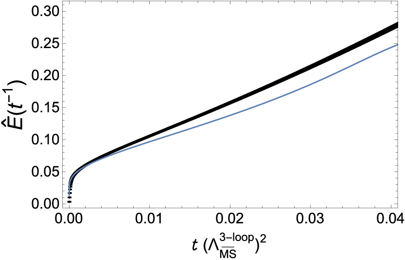
We use lattice data obtained by the FlowQCD collaboration [31, 32].1919 19 We are grateful to Masakiyo Kitazawa for providing us with the numerical data. In Fig. 5, we show the lattice results for for the bare gauge couplings, , , , , and . To show the lattice data in units, we used the relation between and the lattice spacing obtained in Ref. [32].2020 20 We neglect the estimated errors in Ref. [32] in our analysis. We see that the lattice data among different ’s overlap each other in the region . Therefore, we use the lattice data at of the finest lattice spacing ( and , shown by the black line in Fig. 5) regarding it as the continuum limit.2121 21 The selected region satisfies . We adopt such a large scale hierarchy to suppress the finite effect, taking into account that we do not take the continuum limit.

We compare the lattice result in Fig. 5 with the renormalon-free part . To compare them quantitatively, we need the ratio , because our theoretical calculation on the basis of the large- approximation is given in units whereas the lattice results are shown in units. We determine this ratio by requiring the running couplings at one-loop and three-loop to have the same value at , i.e. we impose . (Note that at this scale is determined from since the running coupling at -loop is a function of .) This condition ensures that the calculation at leading-log (LL) matches well with the one at next-to-next-to-LL (NNLL) around the region .2222 22 The LL prediction is the one-loop renormalization group (RG) improvement of the leading-order (LO) prediction. Similarly, the NNLL prediction is the three-loop RG improvement of the NNLO prediction. Due to the matching of the coupling at the lattice cutoff, the difference between these predictions at is of order . This is legitimate because both predictions should be accurate in such a short-distance region. ] The above condition yields .

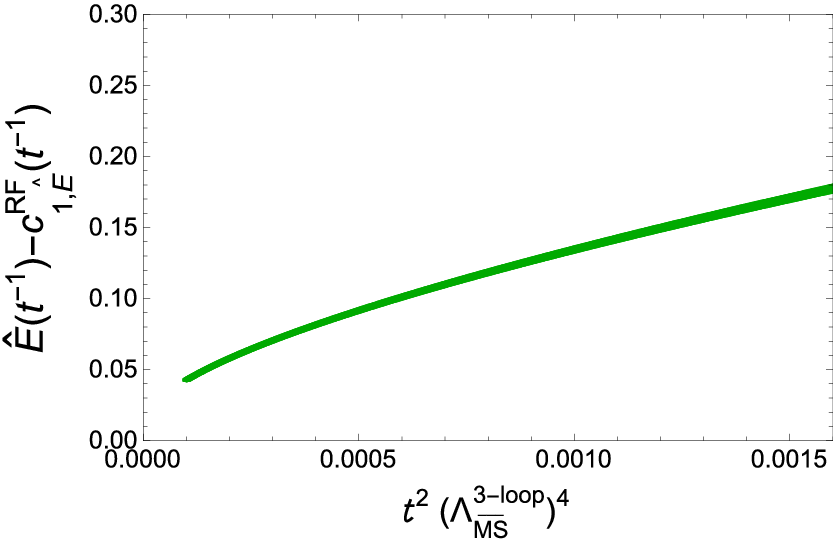

The difference between them, shown in the upper right panel, is expected to have a linear behavior in according to the OPE or small flow time expansion Eq. (3.20). To investigate quantitatively if this is the case or not, in the lower panel, we plot an effective power of the difference defined by , where is the difference and . From the lower panel, it seems that a component with the power smaller than 2 remains in the difference, i.e., the difference does not show behavior. Thus, we cannot extract the gluon condensate, which is the coefficient of the term of the OPE (3.20).
This failure is attributed to the fact that we use the large- approximation to evaluate the Wilson coefficient . In this approximation, the perturbative error does not reach its minimal error (renormalon uncertainty) of , which is expected to be observed in sufficiently large-order perturbative calculations. This is not surprising because the large- approximation takes into account the partial set of the Feynman diagrams and is accurate only at the LL level. In case we do not know a sufficiently large-order result, the difference between nonperturbative (lattice) and perturbative results behaves as rather than .
Although the large- approximation is not sufficient to detect behavior, we now investigate whether such behavior is observed when we use the exact perturbative calculation, which is currently known up to NNLO, namely [30]. In Fig. 7 we compare the NNLL result with the lattice result. The renormalization scale is taken as . We again examine the effective power in of their difference, which turns out to still be smaller than 2. We also show the results with different choices of the renormalization scale but they exhibit similar results.
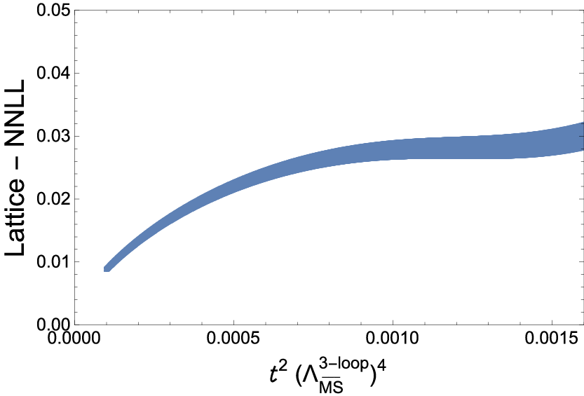

From the above analyses, we conclude that in order to determine the renormalon-free gluon condensate reliably, we need a formulation beyond the large- approximation and also need further higher-order results than are currently available.
References
- [1] J. C. Le Guillou and J. Zinn-Justin, “Large order behavior of perturbation theory,” Amsterdam, Netherlands: North-Holland (1990) 580 p. (Current physics - sources and comments
- [2] G. ’t Hooft, “Can we make sense out of quantum chromodynamics?,” Subnucl. Ser. 15, 943 (1979).
- [3] M. Beneke, Phys. Rept. 317, 1 (1999) doi:10.1016/S0370-1573(98)00130-6 [hep-ph/9807443].
- [4] G. S. Bali, C. Bauer and A. Pineda, Phys. Rev. Lett. 113, 092001 (2014) doi:10.1103/PhysRevLett.113.092001 [arXiv:1403.6477 [hep-ph]].
- [5] G. S. Bali and A. Pineda, AIP Conf. Proc. 1701, 030010 (2016) doi:10.1063/1.4938616 [arXiv:1502.00086 [hep-ph]].
- [6] T. Lee, Phys. Rev. D 82, 114021 (2010) doi:10.1103/PhysRevD.82.114021 [arXiv:1003.0231 [hep-ph]].
- [7] T. Lee, Nucl. Part. Phys. Proc. 258-259, 181 (2015) doi:10.1016/j.nuclphysbps.2015.01.039 [arXiv:1503.07988 [hep-ph]].
- [8] L. Del Debbio, F. Di Renzo and G. Filaci, arXiv:1807.09518 [hep-lat].
- [9] R. Horsley et al., Phys. Rev. D 86, 054502 (2012) doi:10.1103/PhysRevD.86.054502 [arXiv:1205.1659 [hep-lat]].
- [10] G. Mishima, Y. Sumino and H. Takaura, Phys. Rev. D 95, no. 11, 114016 (2017) doi:10.1103/PhysRevD.95.114016 [arXiv:1612.08711 [hep-ph]].
- [11] M. Beneke and V. M. Braun, Phys. Lett. B 348, 513 (1995) doi:10.1016/0370-2693(95)00184-M [hep-ph/9411229].
- [12] D. J. Broadhurst and A. L. Kataev, Phys. Lett. B 315, 179 (1993) doi:10.1016/0370-2693(93)90177-J [hep-ph/9308274].
- [13] P. Ball, M. Beneke and V. M. Braun, Nucl. Phys. B 452, 563 (1995) doi:10.1016/0550-3213(95)00392-6 [hep-ph/9502300].
- [14] G. Mishima, Y. Sumino and H. Takaura, Phys. Lett. B 759, 550 (2016) doi:10.1016/j.physletb.2016.06.010 [arXiv:1602.02790 [hep-ph]].
- [15] M. Neubert, Phys. Rev. D 51, 5924 (1995) doi:10.1103/PhysRevD.51.5924 [hep-ph/9412265].
- [16] M. Beneke and V. A. Smirnov, Nucl. Phys. B 522, 321 (1998) doi:10.1016/S0550-3213(98)00138-2 [hep-ph/9711391].
- [17] V. A. Smirnov, Phys. Lett. B 465, 226 (1999) doi:10.1016/S0370-2693(99)01061-8 [hep-ph/9907471].
- [18] S. L. Adler, Phys. Rev. D 10, 3714 (1974). doi:10.1103/PhysRevD.10.3714
- [19] T. Lee, Phys. Lett. B 711, 360 (2012) doi:10.1016/j.physletb.2012.04.017 [arXiv:1112.4433 [hep-ph]].
- [20] R. Narayanan and H. Neuberger, JHEP 0603, 064 (2006) doi:10.1088/1126-6708/2006/03/064 [hep-th/0601210].
- [21] M. Lüscher, JHEP 1008, 071 (2010) Erratum: [JHEP 1403, 092 (2014)] doi:10.1007/JHEP08(2010)071, 10.1007/JHEP03(2014)092 [arXiv:1006.4518 [hep-lat]].
- [22] M. Lüscher and P. Weisz, JHEP 1102, 051 (2011) doi:10.1007/JHEP02(2011)051 [arXiv:1101.0963 [hep-th]].
- [23] K. Hieda, H. Makino and H. Suzuki, Nucl. Phys. B 918, 23 (2017) doi:10.1016/j.nuclphysb.2017.02.017 [arXiv:1604.06200 [hep-lat]].
- [24] A. Ramos, PoS LATTICE 2014, 017 (2015) doi:10.22323/1.214.0017 [arXiv:1506.00118 [hep-lat]].
- [25] M. Dalla Brida et al. [ALPHA Collaboration], Phys. Rev. Lett. 117, no. 18, 182001 (2016) doi:10.1103/PhysRevLett.117.182001 [arXiv:1604.06193 [hep-ph]].
- [26] H. Suzuki, PTEP 2013, 083B03 (2013) Erratum: [PTEP 2015, 079201 (2015)] doi:10.1093/ptep/ptt059, 10.1093/ptep/ptv094 [arXiv:1304.0533 [hep-lat]].
- [27] H. Makino and H. Suzuki, PTEP 2014, 063B02 (2014) Erratum: [PTEP 2015, 079202 (2015)] doi:10.1093/ptep/ptu070, 10.1093/ptep/ptv095 [arXiv:1403.4772 [hep-lat]].
- [28] H. Takaura, Phys. Lett. B 783, 350 (2018) doi:10.1016/j.physletb.2018.07.014 [arXiv:1712.05435 [hep-ph]].
- [29] Y. Sumino, Phys. Rev. D 76, 114009 (2007) doi:10.1103/PhysRevD.76.114009 [hep-ph/0505034].
- [30] R. V. Harlander and T. Neumann, JHEP 1606, 161 (2016) doi:10.1007/JHEP06(2016)161 [arXiv:1606.03756 [hep-ph]].
- [31] M. Asakawa, T. Hatsuda, T. Iritani, E. Itou, M. Kitazawa and H. Suzuki, arXiv:1503.06516 [hep-lat].
- [32] M. Kitazawa, T. Iritani, M. Asakawa, T. Hatsuda and H. Suzuki, Phys. Rev. D 94, no. 11, 114512 (2016) doi:10.1103/PhysRevD.94.114512 [arXiv:1610.07810 [hep-lat]].