跳到论文正文
W Papers独立论文阅读器 arXiv:1807.09934 论文正文 计算阅读时间 · 0%
引用这篇论文根据当前论文元数据生成,正式投稿前建议核对。


License: arXiv.org perpetual non-exclusive license
arXiv:1807.09934v1 [cs.IT] 26 Jul 2018

The Strongly Asynchronous Massive Access Channel

Sara Shahi, Daniela Tuninetti and Natasha Devroye Affiliation: University of Illinois at Chicago, Chicago IL 60607, USA.
Email: sshahi7, danielat, devroye @uic.edu
Abstract

This paper considers a Strongly Asynchronous and Slotted Massive Access Channel (SAS-MAC) where Kn:=en​νK_{n}:=e^{n\nu} different users transmit a randomly selected message among Mn:=en​RM_{n}:=e^{nR} ones within a strong asynchronous window of length An:=en​αA_{n}:=e^{n\alpha} blocks, where each block lasts nn channel uses. A global probability of error is enforced, ensuring that all the users’ identities and messages are correctly identified and decoded. Achievability bounds are derived for the case that different users have similar channels, the case that users’ channels can be chosen from a set which has polynomially many elements in the blocklength nn, and the case with no restriction on the users’ channels. A general converse bound on the capacity region and a converse bound on the maximum growth rate of the number of users are derived.

I Introduction

In the Internet of Things (IoT) paradigm it is envisioned that many types of devices will be wirelessly connected. A foundational study to understand the fundamental tradeoffs and thus enable the successful deployment of ubiquitous, interconnected wireless network is needed. This new paradigm imposes new traffic patterns on the wireless network. Moreover, devices within such a network often have strict energy consumption constraints, as they are often battery powered sensors transmitting bursts of data very infrequently to an access point. Finally, as the name suggests, these networks must support a huge number of inter-connected devices.

Due to these new network characteristics, we propose a novel communication and multiple-access model: the Strongly Asynchronous Slotted Massive Access (SAS-MAC). In a SAS-MAC, the number of users Kn:=en​νK_{n}:=e^{n\nu} increases exponentially with blocklength nn with occupancy exponent ν≥0\nu\geq 0. Moreover, the users are strongly asynchronous, i.e., they transmit in one randomly chosen time slot within a window of length An:=en​αA_{n}:=e^{n\alpha} blocks, each block of length nn, where α≥0\alpha\geq 0 is the asynchronous exponent. In addition, when active, each user can choose from a set of Mn:=en​RM_{n}:=e^{nR} messages to transmit.All transmissions are sent to an access point and the receiver is required to jointly decode and identify all users. The goal is to characterize the set of all achievable (R,α,ν)(R,\alpha,\nu) triplets.

I-A Past work

Strongly asynchronous communications were first introduced in [1] for synchronization of a single user, and later extended in [2] for synchronization with positive transmission rate.

In [3] the authors of [2] made a brief remark about a “multiple access collision channel” extension of their original single-user model. In this model, any collision of users (i.e., users who happen to transmit in the same block) is assumed to result in output symbols that appear as if generated by noise. The error metric is taken to be the per user probability of error, which is required to be vanishing for all but a vanishing fraction of users. In this scenario, it is fairly easy to quantify the capacity region for the case that the number of users are less than the square root of the asynchronous window length (i.e., in our notation ν<α/2\nu<\alpha/2). However, finding the capacity of the “multiple access collision channel” for global / joint probability of error, as opposed to per user probability of error, is much more complicated and requires novel achievability schemes and novel analysis tools. This is the main subject and contribution of this paper.

Recently, motivated by the emerging machine-to-machine type communications and sensor networks, a large body of work has studied “many-user” versions of classical multiuser channels as pioneered in [4]. In [4] the number of users is allowed to grow linearly with blocklength nn. A full characterization of the capacity of the synchronous Gaussian (random) many access channel was given [4]. In [5], the author studied the synchronous massive random access channel where the total number of users increases linearly with the blocklength nn. However, the users are restricted to use the same codebook and only a per user probability of error is enforced. In the model proposed here, the users are strongly asynchronous, the number of users grow exponentially with blocklength, and we enforce a global probability of error.

Training based synchronization schemes (the use of pilot signals) was proven to be suboptimal for bursty communications in [2]. Rather, one can utilize the users’ statistics at the receiver for synchronization or user identification purposes. The identification problem (defined in [6]) is a classic problem considered in hypothesis testing. In this problem, a finite number of distinct sources each generates a sequence of i.i.d. samples. The problem is to find the underlying distribution of each sample sequence, given the constraint that each sequence is generated by a distinct distribution.

Studies on identification problems all assume a fixed number of sequences. In [7], authors study the Logarithmically Asymptotically Optimal (LAO) Testing of identification problem for a finite number of distributions. In particular, the identification of only two different objects has been studied in detail, and one can find the reliability matrix, which consists of the error exponents of all error types. Their optimality criterion is to find the largest error exponent for a set of error types for given values of the other error type exponents. The same problem with a different optimality criterion was also studied in [8], where multiple, finite sequences were matched to the source distributions. More specifically, the authors in [8] proposed a test for a generalized Neyman-Pearson-like optimality criterion to minimize the rejection probability given that all other error probabilities decay exponentially with a pre-specified slope.

In this paper, we too allow the number of users to increase in the blocklength. We assume that the users are strongly asynchronous and may transmit randomly anytime within a time window that is exponentially large in the blocklength. We require the receiver to recover both the transmitted messages and the users’ identities under a global/joint probability of error criteria. By allowing the number of sequences to grow exponentially with the number of samples, the number of different possibilities (or hypotheses), would be doubly exponential in blocklength and the analysis of the optimal decoder becomes much more challenging than classical (with constant number of distributions) identification problems. These differences in modeling the channel require a number of novel analytical tools.

I-B Contribution

In this paper, we consider the SAS-MAC whose number of users increase exponentially with blocklength nn. In characterizing the capacity of this model, we require its global probability of error to be vanishing. More specifically our contributions are as follows:

  • •

    We define a new massive identification paradigm in which we allow the number of sequences in a classical identification problem to increase exponentially with the sequence blocklength (or sample size). We find asymptotically matching upper and lower bounds on the probability of identification error for this problem. We use this result in our SAS-MAC model to recover the identity of the users.

  • •

    We propose a new achievability scheme that supports strictly positive values of (R,α,ν)(R,\alpha,\nu) for identical channels for the users.

  • •

    We propose a new achievability scheme for the case that the channels of the users are chosen from a set of conditional distributions. The size of the set increases polynomially in the blocklength nn. In this case, the channel statistics themselves can be used for user identification.

  • •

    We propose a new achievability scheme without imposing any restrictive assumptions on the users’ channels. We show that strictly positive (R,α,ν)(R,\alpha,\nu) are possible.

  • •

    We propose a novel converse bound for the capacity of the SAS-MAC.

  • •

    We show that for ν>α\nu>\alpha, not even reliable synchronization is possible.

These results were presented in parts in [9, 10, 11].

I-C Paper organization

In Section II we introduce our massive identification model and present a technical theorem (Theorem 1) that will be needed later on in the proof of Theorem 3. In Section III we introduce the SAS-MAC model and in Section IV we present our main results. More specifically, we introduce different achievability schemes for different scenarios and a converse technique to derive an upper bound on the capacity of the SAS-MAC. Finally, Section V concludes the paper. Some proofs may be found in the Appendix.

I-D Notation

Capital letters represent random variables that take on lower case letter values in calligraphic letter alphabets. The notation an≐en​ba_{n}\doteq e^{nb} means limn→∞log⁡ann=b\lim_{n\to\infty}\frac{\log a_{n}}{n}=b. We write [M:N][M:N], where M,N∈ℤ,M≤NM,N\in\mathbb{Z},M\leq N, to denote the set {M,M+1,…,N}\{M,M+1,\ldots,N\}, and [K]:=[1:K][K]:=[1:K]. We use yjn:=[yj,1,…,yj,n]y_{j}^{n}:=[y_{j,1},...,y_{j,n}], and simply yny^{n} instead of y1ny_{1}^{n}. The binary entropy function is defined by h⁡(p):=−p​log⁡(p)−(1−p)​log⁡(1−p)h(p):=-p\log(p)-(1-p)\log(1-p).

II Massive Identification Problem

We first introduce notation specifically used in this Section and then introduce our model and results.

II-A Notation

When all elements of the random vector XnX^{n} are generated i.i.d according to distribution PP, we denote it as Xn[1]∼i.i.dPX^{n}\mathrel{\overset{\text{i.i.d}}{[1]{$\sim$}}}P. We use SnS_{n}, where |Sn|=n!|S_{n}|=n!, to denote the set of all possible permutations of a set of nn elements. For a permutation σ∈Sn\sigma\in S_{n}, σi\sigma_{i} denotes the ii-th element of the permutation. ⌊x⌋r\lfloor x\rfloor_{r} is used to denote the remainder of xx divided by rr. Kk​(a1,…,a(k2))K_{k}\left(a_{1},\ldots,a_{\binom{k}{2}}\right) is the complete graph with kk nodes with edge index i∈[(k2)]i\in[\binom{k}{2}] and edge weights ai,i∈[(k2)]a_{i},\ i\in[\binom{k}{2}]. We may drop the edge argument and simply write KkK_{k} when the edge specification is not needed. A cycle cc of length rr in KkK_{k} may be interchangeably defined by a vector of vertices as c(v)=[v1,…,vr]c^{(v)}=\left[v_{1},\ldots,v_{r}\right] or by a set of edges c(e)={a1,…,ar}c^{(e)}=\left\{a_{1},\ldots,a_{r}\right\} where aia_{i} is the edge between (vi,vi+1),∀i∈[r−1](v_{i},v_{i+1}),\forall i\in[r-1] and ara_{r} is that between (vr,v1)(v_{r},v_{1}). With this notation, c(v)​(i)c^{(v)}(i) is then used to indicate the ii-th vertex of the cycle cc. Ck(r)C^{(r)}_{k} is used to denote the set of all cycles of length rr in the complete graph Kk​(a1,…,a(k2))K_{k}\left(a_{1},\ldots,a_{\binom{k}{2}}\right). The cycle gain, denoted by G⁡(c)G(c), for cycle c={a1,…,ar}∈Ck(r)c=\left\{a_{1},\ldots,a_{r}\right\}\in C^{(r)}_{k} is the product of the edge weights within the cycle cc, i.e., G⁡(c)=∏i=1rai,∀ai∈cG(c)=\prod_{i=1}^{r}a_{i},\ \forall a_{i}\in c.

The Bhatcharrya distance between P1P_{1} and P2P_{2} is denoted by B⁡(P1,P2):=∑x∈𝒳P1​(x)​P2​(x)B(P_{1},P_{2}):=\sum_{x\in\mathcal{X}}\sqrt{P_{1}(x)P_{2}(x)}.

II-B Problem Formulation

Let P:={P1,…,PA},Pi∈𝒫𝒳,∀i∈[A]P:=\{P_{1},\ldots,P_{A}\},P_{i}\in\mathcal{P}_{\mathcal{X}},\forall i\in[A] consist of AA distinct distributions and also let Σ\Sigma be uniformly distributed over SAS_{A}, the set of permutations of AA elements. In addition, assume that we have AA independent random vectors {X1n,X2n,…,XAn}\{X_{1}^{n},X_{2}^{n},\ldots,X_{A}^{n}\} of length nn each. For σ\sigma, a realization of Σ\Sigma, assign the distribution PσinP_{\sigma_{i}}^{n} to the random vector Xin,∀i∈[A]X_{i}^{n},\forall i\in[A]. After observing a sample xn​A=[x1n,…,xAn]x^{nA}=[x_{1}^{n},\ldots,x_{A}^{n}] of the random vector Xn​A=[X1n,…,XAn]X^{nA}=\left[X_{1}^{n},\ldots,X_{A}^{n}\right], we would like to identify Pσi,∀i∈[A]P_{\sigma_{i}},\forall i\in[A]. More specifically, we are interested in finding a permutation σ^:𝒳n​A→SA\hat{\sigma}:\mathcal{X}^{nA}\to S_{A} to indicate that Xin[1]∼i.i.dPσ^i,∀i∈[A]X_{i}^{n}\mathrel{\overset{\text{i.i.d}}{[1]{$\sim$}}}P_{\hat{\sigma}_{i}},\ \forall i\in[A]. Let Σ^=σ^​(Xn​A)\hat{\Sigma}=\hat{\sigma}(X^{nA}).

The average probability of error for the set of distributions PP is given by

Pe(n)\displaystyle P_{e}^{(n)} =ℙ[Σ^≠Σ]\displaystyle=\mathbb{P}\left[\hat{\Sigma}\neq\Sigma\right]
=1(A)!∑σ∈SAℙ[Σ^≠σ|Xin[1]∼i.i.dPσi,∀i∈[A]]\displaystyle=\frac{1}{(A)!}\sum_{\sigma\in S_{A}}\mathbb{P}\left[\hat{\Sigma}\neq\sigma|X_{i}^{n}\mathrel{\overset{\text{i.i.d}}{[1]{$\sim$}}}P_{\sigma_{i}},\forall i\in[A]\right]
=ℙ[Σ^≠(1,2,…,A)|Xin[1]∼i.i.dPi,∀i∈[A]].\displaystyle=\mathbb{P}\left[\hat{\Sigma}\neq\left(1,2,\ldots,A\right)\big|X_{i}^{n}\mathrel{\overset{\text{i.i.d}}{[1]{$\sim$}}}P_{i},\forall i\in[A]\right].

We say that a set of distributions PP is identifiable if limn→∞Pe(n)→0\lim_{n\to\infty}P_{e}^{(n)}\to 0.

II-C Condition for Identifiability

In Theorem 1 we characterize the relation between the number of distributions and the pairwise distance of the distributions for reliable identification. Moreover, we introduce and use a novel graph theoretic technique in the proof of Theorem 1 to analyze the optimal Maximum Likelihood decoder.

Theorem 1.

A sequence of distributions P={P1,…,PAn}P=\{P_{1},\ldots,P_{A_{n}}\} is identifiable iff

limn→∞∑1≤i<j≤Ane−2​n​B​(Pi,Pj)=0.\displaystyle\lim_{n\to\infty}\sum_{\begin{subarray}{c}1\leq i<j\leq A_{n}\end{subarray}}e^{-2nB(P_{i},P_{j})}=0. (1)

The rest of this section contains the proof. To prove Theorem 1, we provide upper and lower bounds on the probability of error in the following subsections.

II-D Upper bound on the probability of identification error

We use the optimal Maximum Likelihood (ML) decoder, which minimizes the average probability of error, given by

σ^​(x1n,…,xAnn):=arg⁡max⁡∑i=1Anσ∈SAn⁡log⁡(Pσi​(xin)),\displaystyle\hat{\sigma}(x_{1}^{n},\ldots,x_{A_{n}}^{n}):=\arg\max_{\sigma\in S_{A_{n}}}\sum_{i=1}^{A_{n}}\log\left(P_{\sigma_{i}}\left(x_{i}^{n}\right)\right), (2)

where Pσi​(xin)=∏t=1nPσi​(xi,t)P_{\sigma_{i}}\left(x_{i}^{n}\right)=\prod_{t=1}^{n}P_{\sigma_{i}}\left(x_{i,t}\right). The average probability of error associated with the ML decoder can also be written as

Pe(n)\displaystyle P_{e}^{(n)} =ℙ⁡[Σ^≠[An]|H^]\displaystyle=\mathbb{P}\left[\hat{\Sigma}\neq[A_{n}]\big|\widehat{H}\right]
=ℙ⁡[⋃σ^≠[An]Σ^=σ^|H^]\displaystyle=\mathbb{P}\left[\bigcup_{\hat{\sigma}\neq[A_{n}]}\hat{\Sigma}=\hat{\sigma}\big|\widehat{H}\right]
=ℙ[⋃r=2An⋃σ^:{∑i=1An𝟙{σ^i≠i}=r}Σ^=σ^|H^]\displaystyle=\mathbb{P}\left[\bigcup_{r=2}^{A_{n}}\bigcup_{\begin{subarray}{c}\hat{\sigma}:\\ \left\{\sum_{i=1}^{A_{n}}\mathbbm{1}_{\{\hat{\sigma}_{i}\neq i\}}=r\right\}\end{subarray}}\hat{\Sigma}=\hat{\sigma}\big|\widehat{H}\right] (3)
=ℙ[⋃r=2An⋃σ^:{∑i=1An𝟙{σ^i≠i}=r}∑i=1AnlogPσ^i​(Xin)Pi​(Xin)≥0|H^],\displaystyle=\mathbb{P}\Bigg[\bigcup_{r=2}^{A_{n}}\bigcup_{\begin{subarray}{c}\hat{\sigma}:\\ \left\{\sum_{i=1}^{A_{n}}\mathbbm{1}_{\{\hat{\sigma}_{i}\neq i\}}=r\right\}\end{subarray}}\sum_{i=1}^{A_{n}}\log\frac{P_{\hat{\sigma}_{i}}\left(X_{i}^{n}\right)}{P_{i}\left(X_{i}^{n}\right)}\geq 0\big|\widehat{H}\Bigg], (4)

where H^:={Xin[1]∼i.i.dPi,∀i∈[An]}\widehat{H}:=\left\{X_{i}^{n}\mathrel{\overset{\text{i.i.d}}{[1]{$\sim$}}}P_{i},\forall i\in[A_{n}]\right\} and where (3) is due to the requirement that each sequence is distributed according to a distinct distribution and hence the number of incorrect distributions ranges from [2:An][2:A_{n}]. In order to avoid considering the same set of error events multiple times, we incorporate a graph theoretic interpretation of {∑i=1An𝟙{Σ^i≠i}=r}\left\{\sum_{i=1}^{A_{n}}\mathbbm{1}_{\{\hat{\Sigma}_{i}\neq i\}}=r\right\} in (4) which is used to denote the fact that we have identified rr distributions incorrectly. Consider the two sequences [i1,…,ir][i_{1},\ldots,i_{r}] and [σ^i1,…,σ^ir][\hat{\sigma}_{i_{1}},\ldots,\hat{\sigma}_{i_{r}}] for which we have

{∑i=1An𝟙{σ^i≠i}=∑j=1r𝟙{σ^ij≠ij}=r}.\left\{\sum_{i=1}^{A_{n}}\mathbbm{1}_{\{\hat{\sigma}_{i}\neq i\}}=\sum_{j=1}^{r}\mathbbm{1}_{\{\hat{\sigma}_{i_{j}}\neq i_{j}\}}=r\right\}.

These two sequences in (4) in fact indicate the event that we have (incorrectly) identified Xijn[1]∼i.i.dPσ^ijX_{i_{j}}^{n}\mathrel{\overset{\text{i.i.d}}{[1]{$\sim$}}}P_{\hat{\sigma}_{i_{j}}} instead of the (true) distribution Xijn[1]∼i.i.dPij,∀j∈[r]X_{i_{j}}^{n}\mathrel{\overset{\text{i.i.d}}{[1]{$\sim$}}}P_{{i_{j}}},\forall j\in[r]. For a complete graph KAnK_{A_{n}}, the set of edges between ((i1,σ^i1),…,(ir,σ^ir))\left((i_{1},\hat{\sigma}_{i_{1}}),\ldots,(i_{r},\hat{\sigma}_{i_{r}})\right) in KAnK_{A_{n}} would produce a single cycle of length rr or a set of disjoint cycles with total length rr. However, we should note that in the latter case where the sequence of edges construct a set of (lets say of size LL) disjoint cycles (each with some length r~l\tilde{r}_{l} for r~l<r\tilde{r}_{l}<r such that ∑l=1Lr~l=r\sum_{l=1}^{L}\tilde{r}_{l}=r), then those cycles and their corresponding sequences are already taken into account in the (union of) set of r~l\tilde{r}_{l} error events.

As an example, assume An=4A_{n}=4 and consider the error event

log⁡P2​(X1n)P1​(X1n)+log⁡P1​(X2n)P2​(X2n)+log⁡P4​(X3n)P3​(X3n)+log⁡P3​(X4n)P4​(X4n)≥0,\log\frac{P_{2}(X_{1}^{n})}{P_{1}(X_{1}^{n})}+\log\frac{P_{1}(X_{2}^{n})}{P_{2}(X_{2}^{n})}+\log\frac{P_{4}(X_{3}^{n})}{P_{3}(X_{3}^{n})}+\log\frac{P_{3}(X_{4}^{n})}{P_{4}(X_{4}^{n})}\geq 0,

which corresponds to the (error) event of choosing [σ^1,σ^2,σ^3,σ^4]=[2,1,4,3][\hat{\sigma}_{1},\hat{\sigma}_{2},\hat{\sigma}_{3},\hat{\sigma}_{4}]=[2,1,4,3] over [1,2,3,4][1,2,3,4] with r=4r=4 errors. In the graph representation, this gives two cycles of length 22 each, which correspond to

{logP2​(X1n)P1​(X1n)+logP1​(X2n)P2​(X2n)≥0}∩{logP4​(X3n)P3​(X3n)+logP3​(X4n)P4​(X4n)≥0},\displaystyle\left\{\log\frac{P_{2}(X_{1}^{n})}{P_{1}(X_{1}^{n})}+\log\frac{P_{1}(X_{2}^{n})}{P_{2}(X_{2}^{n})}\geq 0\ \right\}\cap\left\{\log\frac{P_{4}(X_{3}^{n})}{P_{3}(X_{3}^{n})}+\log\frac{P_{3}(X_{4}^{n})}{P_{4}(X_{4}^{n})}\geq 0\right\},

and are already accounted for in the events

{[σ^1,σ^2,σ^3,σ^4]=[2,1,3,4]}∪{[σ^1,σ^2,σ^3,σ^4]=[1,2,4,3]}\left\{[\hat{\sigma}_{1},\hat{\sigma}_{2},\hat{\sigma}_{3},\hat{\sigma}_{4}]=[2,1,3,4]\right\}\cup\left\{[\hat{\sigma}_{1},\hat{\sigma}_{2},\hat{\sigma}_{3},\hat{\sigma}_{4}]=[1,2,4,3]\right\}

with r=2r=2.

As the result, in order to avoid double counting, in evaluating (4) for each rr we should only consider the sets of sequences which produce a single cycle of length rr.

Before proceeding further, we define the edge weights for a complete weighted graph

KAn​(a(1,2),…​a(Kn,1)).K_{A_{n}}(a_{(1,2)},\ldots a_{(K_{n},1)}).

In particular, we define a(i,j):=e−n​B​(Pi,Pj)a_{(i,j)}:=e^{-nB(P_{i},P_{j})} to be the edge weight between vertices (i,j)(i,j) in the complete graph KAnK_{A_{n}} shown in Fig. 1.

Fig. 1: Complete graph KAnK_{A_{n}} with edge weight e−n​B​(Pi,Pj)e^{-nB(P_{i},P_{j})} for every pair of vertices i≠j∈[Kn]i\neq j\in[K_{n}].

Hence, we can upper bound the probability of error in (4) as

Pe(n)\displaystyle P_{e}^{(n)} ≤∑r=2An∑c∈CAn(r)ℙ⁡[∑i=1rlog⁡P⌊c(v)​(i+1)⌋r​(Xc(v)​(i)n)Pc(v)​(i)​(Xc(v)​(i)n)≥0|H^]\displaystyle\leq\sum_{r=2}^{A_{n}}\sum_{\begin{subarray}{c}c\in C^{(r)}_{A_{n}}\end{subarray}}\mathbb{P}\left[\sum_{i=1}^{r}\log\frac{P_{\lfloor c^{(v)}(i+1)\rfloor_{r}}\left(X^{n}_{c^{(v)}(i)}\right)}{P_{c^{(v)}(i)}\left(X^{n}_{c^{(v)}(i)}\right)}\geq 0|\widehat{H}\right]
≤∑r=2An∑c∈CAn(r)e−n∑i=1rB(Pc(v)​(i),Pc(v)​(⌊i+1⌋r))\displaystyle\leq\sum_{r=2}^{A_{n}}\sum_{\begin{subarray}{c}c\in C^{(r)}_{A_{n}}\end{subarray}}e^{-n\sum_{i=1}^{r}B(P_{c^{(v)}(i)},P_{c^{(v)}(\lfloor i+1\rfloor_{r})})} (5)
=∑r=2An∑c∈CAn(r)G⁡(c),\displaystyle=\sum_{r=2}^{A_{n}}\sum_{c\in C_{A_{n}}^{(r)}}G(c), (6)

where rr enumerates the number of incorrect matchings and where c⁡(i)c(i) is the ii-th vertex in the cycle cc. In (6), we have leveraged the fact that e−n​B​(Pi,Pj)e^{-nB(P_{i},P_{j})} is the edge weight between vertices (i,j)(i,j) in the complete graph KAnK_{A_{n}} and hence G(c)=e−n∑i=1rB(Pc(v)​(i),Pc(v)​(⌊i+1⌋r))G(c)=e^{-n\sum_{i=1}^{r}B(P_{c^{(v)}(i)},P_{c^{(v)}(\lfloor i+1\rfloor_{r})})} is the gain of cycle cc. The inequality in (5) is by

ℙ⁡[∑i=1rlog⁡P⌊c(v)​(i+1)⌋r​(Xc(v)​(i)n)Pc(v)​(i)​(Xc(v)​(i)n)≥0|H^]\displaystyle\mathbb{P}\left[\sum_{i=1}^{r}\log\frac{P_{\lfloor c^{(v)}(i+1)\rfloor_{r}}\left(X^{n}_{c^{(v)}(i)}\right)}{P_{c^{(v)}(i)}\left(X^{n}_{c^{(v)}(i)}\right)}\geq 0|\widehat{H}\right]
≤exp⁡{n​inftlog⁡𝔼⁡[∏i=1r(Pc(v)​(⌊i+1⌋r)​(Xc⁡(i)n)Pc(v)​(i)​(Xc⁡(i)n))t]}\displaystyle\leq\exp\left\{n\inf_{t}\log\mathbb{E}\left[\prod_{i=1}^{r}\left(\frac{P_{c^{(v)}(\lfloor i+1\rfloor_{r})}\left(X^{n}_{c(i)}\right)}{P_{c^{(v)}(i)}\left(X^{n}_{c(i)}\right)}\right)^{t}\right]\right\}
≤exp⁡{n​∑i=1rlog⁡𝔼⁡[(Pc(v)​(⌊i+1⌋r)​(Xc⁡(i)n)Pc(v)​(i)​(Xc⁡(i)n))1/2]}\displaystyle\leq\exp\left\{n\sum_{i=1}^{r}\log\mathbb{E}\left[\left(\frac{P_{c^{(v)}(\lfloor i+1\rfloor_{r})}\left(X^{n}_{c(i)}\right)}{P_{c^{(v)}(i)}\left(X^{n}_{c(i)}\right)}\right)^{1/2}\right]\right\} (7)
=exp{−n∑i=1rB(Pc(v)​(i),Pc(v)​(⌊i+1⌋r))}.\displaystyle=\exp\left\{-n\sum_{i=1}^{r}B(P_{c^{(v)}(i)},P_{c^{(v)}(\lfloor i+1\rfloor_{r})})\right\}.

The fact that we used t=1/2t=1/2 in (7) instead of finding the exact optimizing tt, comes from the fact that t=1/2t=1/2 is the optimal choice for r=2r=2 and as we will see later, the rest of the error events are dominated by the set of only 22 incorrectly identified distributions. This can be seen as follows for X1n[1]∼i.i.dP1,X2n[1]∼i.i.dP2X_{1}^{n}\mathrel{\overset{\text{i.i.d}}{[1]{$\sim$}}}P_{1},X_{2}^{n}\mathrel{\overset{\text{i.i.d}}{[1]{$\sim$}}}P_{2}

ℙ[logP1​(X2n)P2​(X2n)+logP2​(X1n)P1​(X1n)≥0]\displaystyle\mathbb{P}\left[\log\frac{P_{1}(X^{n}_{2})}{P_{2}(X^{n}_{2})}+\log\frac{P_{2}(X_{1}^{n})}{P_{1}(X_{1}^{n})}\geq 0\right]
=∑P^1,P2^:∑x∈𝒳P^1​(x)​log⁡P2​(x)P1​(x)+P2^​(y)​log⁡P1​(x)P2​(x)≥0exp{nD(P^1∥P1)−nD(P^2∥P2)}\displaystyle=\sum_{\begin{subarray}{c}\hat{P}_{1},\hat{P_{2}}:\\ \sum_{x\in\mathcal{X}}\hat{P}_{1}(x)\log\frac{P_{2}(x)}{P_{1}(x)}+\\ \hat{P_{2}}(y)\log\frac{P_{1}(x)}{P_{2}(x)}\geq 0\end{subarray}}\exp\left\{nD\left(\hat{P}_{1}\parallel P_{1}\right)\!-\!nD\left(\hat{P}_{2}\parallel P_{2}\right)\!\right\}
≐e−nD(P~∥P1)−nD(P~∥P2)=e−2​n​B​(P1,P2),\displaystyle\doteq e^{-nD\left(\tilde{P}\parallel P_{1}\right)-nD\left(\tilde{P}\parallel P_{2}\right)}=e^{-2nB(P_{1},P_{2})}, (8)

where P~\tilde{P} in the first equality in (8), by using the Lagrangian method, can be shown to be equal to P~​(x)=P1​(x)​P2​(x)∑x′P1​(x′)​P2​(x′)\tilde{P}(x)=\frac{\sqrt{P_{1}(x)P_{2}(x)}}{\sum_{x^{\prime}}\sqrt{P_{1}(x^{\prime})P_{2}(x^{\prime})}} and subsequently the second inequality in (8) is proved.

In order to calculate the expression in (6), we use the following graph theoretic Lemma, the proof of which is given in Appendix -A.

Lemma 1.

In a complete graph Kk​(a1,…,ank)K_{k}\left(a_{1},\ldots,a_{n_{k}}\right) and for the set of cycles of length rr, 𝒞k(r)={c1,…​cNr,k}\mathcal{C}_{k}^{(r)}=\{c_{1},\ldots c_{N_{r,k}}\}, we have

1Nr,k​(G⁡(c1)+…​G​(cNr,k))\displaystyle\frac{1}{N_{r,k}}\left(G(c_{1})+\ldots G(c_{N_{r,k}})\right) ≤(a12+…+ank2nk)r2\displaystyle\leq\left(\frac{a_{1}^{2}+\ldots+a_{n_{k}}^{2}}{n_{k}}\right)^{\frac{r}{2}}

where Nr,k,nkN_{r,k},n_{k} are the number of cycles of length rr and the number of edges in the complete graph KkK_{k}, respectively.

By Lemma 1 and (6) we prove in Appendix -B that the upper bound on the probability of error Pe(n)P_{e}^{(n)} goes to zero if

limn→∞∑1≤i<j≤Ane−2​n​B​(Pi,Pj)=0.\displaystyle\lim_{n\to\infty}\sum_{\begin{subarray}{c}1\leq i<j\leq A_{n}\end{subarray}}e^{-2nB(P_{i},P_{j})}=0. (9)

As a result of Lemma 1, it can be seen from (88) that the sum of probabilities that r≥3r\geq 3 distributions are incorrectly identified is dominated by the probability that only r=2r=2 distributions are incorrectly identified. This shows that the most probable error event is indeed an error event with two wrong distributions.

II-E Lower bound on the probability of identifiability error

For our converse, we use the optimal ML decoder, and as a lower bound to the probability of error in (4), we only consider the set of error events with only two incorrect distributions, i.e., the set of events with r=2r=2. In this case we have

Pe(n)\displaystyle P_{e}^{(n)} ≥ℙ⁡[⋃1≤i<j≤Anlog⁡Pi​(Xjn)Pj​(Xjn)+log⁡Pj​(Xin)Pi​(Xin)≥0|H^]\displaystyle\geq\mathbb{P}\left[\bigcup_{\begin{subarray}{c}1\leq i<j\leq A_{n}\end{subarray}}\log\frac{P_{i}(X^{n}_{j})}{P_{j}(X^{n}_{j})}+\log\frac{P_{j}(X_{i}^{n})}{P_{i}(X_{i}^{n})}\geq 0|\widehat{H}\right]
≥(∑1≤i<j≤Anℙ⁡[ξi,j])2∑(i,j),(j,k)(i,j)≠(l,k)i≠j,l≠kℙ⁡[ξi,j,ξk,l],\displaystyle\geq\frac{\left(\sum_{\begin{subarray}{c}1\leq i<j\leq A_{n}\end{subarray}}\mathbb{P}\left[\xi_{i,j}\right]\right)^{2}}{\sum_{\begin{subarray}{c}(i,j),(j,k)\\ (i,j)\neq(l,k)\\ i\neq j,l\neq k\end{subarray}}\mathbb{P}[\xi_{i,j},\xi_{k,l}]}, (10)

where (10) is by [12] and where

ξi,j:={log⁡PiPj​(Xjn)+log⁡PjPi​(Xin)≥0|H^}.\displaystyle\xi_{i,j}:=\left\{\log\frac{P_{i}}{P_{j}}(X^{n}_{j})+\log\frac{P_{j}}{P_{i}}(X_{i}^{n})\geq 0|\widehat{H}\right\}. (11)

We prove in Appendix -C that a lower bound on Pe(n)P_{e}^{(n)} is given by

Pe(n)≥\displaystyle P_{e}^{(n)}\geq (∑1≤i<j≤Ane−2​n​B​(Pi,Pj))2∑i,j,ke−n​B​(Pi,Pj)−n​B​(Pi,Pk)−n​B​(Pk,Pj)+(∑i,je−2​n​B​(Pi,Pj))2\displaystyle\frac{\left(\sum_{1\leq i<j\leq A_{n}}e^{-2nB(P_{i},P_{j})}\right)^{2}}{\sum\limits_{i,j,k}e^{-nB(P_{i},P_{j})-nB(P_{i},P_{k})-nB(P_{k},P_{j})}\!+\!\left(\sum\limits_{i,j}e^{-2nB(P_{i},P_{j})}\!\right)^{2}} (12)
≥(∑i,je−2​n​B​(Pi,Pj))28​(∑1≤i<j≤Ane−2​n​B​(Pi,Pj))32+(∑1≤i<j≤Ane−2​n​B​(Pi,Pj))2\displaystyle\geq\frac{\left(\sum_{i,j}e^{-2nB(P_{i},P_{j})}\right)^{2}}{8\left(\sum\limits_{1\leq i<j\leq A_{n}}\!\!\!e^{-2nB(P_{i},P_{j})}\right)^{\!\frac{3}{2}}\!\!\!+\left(\sum\limits_{1\leq i<j\leq A_{n}}e^{-2nB(P_{i},P_{j})}\right)^{2}} (13)
=∑1≤i<j≤Ane−2​n​B​(Pi,Pj)8+∑1≤i<j≤Ane−2​n​B​(Pi,Pj),\displaystyle=\frac{\sqrt{\sum_{1\leq i<j\leq A_{n}}e^{-2nB(P_{i},P_{j})}}}{8+\sqrt{\sum_{1\leq i<j\leq A_{n}}e^{-2nB(P_{i},P_{j})}}}, (14)

where (13) is by Lemma 1. As it can be seen from (14), if limn→∞∑1≤i<j≤Ane−2​n​B​(Pi,Pj)≠0\lim_{n\to\infty}\sum_{\begin{subarray}{c}1\leq i<j\leq A_{n}\end{subarray}}e^{-2nB(P_{i},P_{j})}\neq 0, the probability of error is bounded away from zero. As a result, we have to have

limn→∞∑1≤i<j≤Ane−2​n​B​(Pi,Pj)=0,\lim_{n\to\infty}\sum_{\begin{subarray}{c}1\leq i<j\leq A_{n}\end{subarray}}e^{-2nB(P_{i},P_{j})}=0,

which also matches our upper bound on the probability of error in (89).

Remark 1.

As it is clear from the result of Theorem 1, when AnA_{n} is a constant or grows polynomially with nn, the sequence of distributions in PP are always identifiable and the probability of error in the identification problem decays to zero as the blocklength nn goes to infinity. The interesting aspect of Theorem 1 is in the regime that AnA_{n} increases exponentially with the blocklength.

Having proved the criterion for identifiability of a massive number of distributions in Theorem 1, we move on to the SAS-MAC problem. We use the result of Theorem 1 to identify the massive number of users by their induced probability distribution at the receiver.

III SAS-MAC problem

We first introduce the special notation used in the SAS-MAC and then formally define the problem.

III-A Special Notation

A stochastic kernel / transition probability / channel from 𝒳\mathcal{X} to 𝒴\mathcal{Y} is denoted by Q⁡(y|x),∀(x,y)∈𝒳×𝒴Q(y|x),\forall(x,y)\in\mathcal{X}\times\mathcal{Y}, and the output marginal distribution induced by P∈𝒫𝒳P\in\mathcal{P}_{\mathcal{X}} through the channel QQ as

[P​Q]​(y):=∑x∈𝒳P⁡(x)​Q​(y|x),∀y∈𝒴,\displaystyle[PQ](y):=\sum_{x\in\mathcal{X}}P(x)Q(y|x),\forall y\in\mathcal{Y}, (15)

where 𝒫𝒳\mathcal{P}_{\mathcal{X}} is the space of all distributions on 𝒳\mathcal{X}. We define the shorthand notation

Qx​(y)\displaystyle Q_{x}(y) :=Q⁡(y|x),∀y∈𝒴.\displaystyle:=Q(y|x),\forall y\in\mathcal{Y}. (16)

For a MAC channel Q⁡(y|x1,…,xK),∀(x1,…,xK,y)∈𝒳1×…×𝒳K×𝒴Q(y|x_{1},\ldots,x_{K}),\forall(x_{1},\ldots,x_{K},y)\in\mathcal{X}_{1}\times\ldots\times\mathcal{X}_{K}\times\mathcal{Y}, we define the shorthand notation

QS​(y|xS)\displaystyle Q_{S}\left(y|x_{S}\right) :=Q(y|xS,⋆Sc),∀S⊆[K],\displaystyle:=Q(y|x_{S},\star_{S^{c}}),\forall S\subseteq[K], (17)

to indicate that users indexed by SS transmit xi,∀i∈Sx_{i},\forall i\in S, and users indexed by ScS^{c} transmit their respective idle symbol ⋆j,∀j∈Sc=[K]\S\star_{j},\forall j\in S^{c}=[K]\backslash S. When |S|=1|S|=1, we use

Qi(y|xi):=Q{i}(y|xi)=Q(y|⋆1,…,⋆i−1,xi,⋆i+1,…,⋆K),Q_{i}(y|x_{i}):=Q_{\{i\}}(y|x_{i})=Q(y|\star_{1},\ldots,\star_{i-1},x_{i},\star_{i+1},\ldots,\star_{K}),

and when |S|=0|S|=0, we use

Q⋆(y):=Q(y|⋆1,…⋆K).Q_{\star}(y):=Q(y|\star_{1},\ldots\star_{K}).

The empirical distribution of a sequence xnx^{n} is

P^xn(a):=1n𝒩(a|xn)=1n∑i=1n𝟙{xi=a},∀a∈𝒳,\displaystyle\widehat{P}_{x^{n}}(a):=\frac{1}{n}\mathcal{N}(a|x^{n})=\frac{1}{n}\sum_{i=1}^{n}\mathbbm{1}_{\{x_{i}=a\}},\forall a\in\mathcal{X}, (18)

where 𝒩⁡(a|xn)\mathcal{N}(a|x^{n}) denotes the number of occurrences of letter a∈𝒳a\in\mathcal{X} in the sequence xnx^{n}; when using (18) the target sequence xnx^{n} is usually clear from the context so we may drop the subscript xnx^{n} in P^xn​(⋅)\widehat{P}_{x^{n}}(\cdot). The PP-type set and the VV-shell of the sequence xnx^{n} are defined, respectively, as

T⁡(P)\displaystyle T(P) :={xn:𝒩(a|xn)=nP(a),∀a∈𝒳},\displaystyle:=\left\{x^{n}:\mathcal{N}(a|x^{n})=nP(a),\forall a\in\mathcal{X}\right\}, (19)
TV​(xn)\displaystyle T_{V}(x^{n}) :={yn:𝒩(a,b|xn,yn)𝒩⁡(a|xn)=V(b|a),∀(a,b)∈(𝒳,𝒴)},\displaystyle:=\left\{y^{n}\!:\!\frac{\mathcal{N}\left(a,b|x^{n},y^{n}\right)}{\mathcal{N}(a|x^{n})}=V(b|a),\forall(a,b)\in(\mathcal{X},\mathcal{Y})\right\}, (20)

where 𝒩(a,b|xn,yn)=∑i=1n𝟙{xi=ayi=b}\mathcal{N}(a,b|x^{n},y^{n})=\sum_{i=1}^{n}\mathbbm{1}_{\left\{\begin{subarray}{c}x_{i}=a\\ y_{i}=b\end{subarray}\right\}} is the number of joint occurrences of (a,b)(a,b) in the pair of sequences (xn,yn)(x^{n},y^{n}).

We use D(P1∥P2)D(P_{1}\parallel P_{2}) to denote the Kullback Leibler divergence between distribution P1P_{1} and P2P_{2}, and D(Q1∥Q2|P):=∑x,y∈𝒳×𝒴P(x)Q1(y|x)logQ1​(y|x)Q2​(y|x)D(Q_{1}\parallel Q_{2}|P):=\sum_{x,y\in\mathcal{X}\times\mathcal{Y}}P(x)Q_{1}(y|x)\log\frac{Q_{1}(y|x)}{Q_{2}(y|x)} for the conditional Kullback Leibler divergence. We let I(P,Q)=D(Q∥[PQ]|P)I(P,Q)=D(Q\parallel[PQ]|P) denote the mutual information between random variable (X,Y)(X,Y) with joint distribution PX,Y​(x,y)=P⁡(x)​Q​(y|x)P_{X,Y}(x,y)=P(x)Q(y|x).

III-B SAS-MAC Problem Formulation

Let MM be the number of messages, AA be the number of blocks, and KK be the number of users. An (M,A,K,n,ϵ)(M,A,K,n,\epsilon) code for the SAS-MAC consists of:

  • •

    A message set [M][M], for each user i∈[K]i\in[K], from which messages are chosen uniformly at random and are independent across users.

  • •

    An encoding function fi:[M]→𝒳nf_{i}:[M]\to\mathcal{X}^{n}, for each user i∈[K]i\in[K]. We define

    xin​(m):=fi​(m).\displaystyle x_{i}^{n}(m):=f_{i}(m). (21)

    Each user i∈[K]i\in[K] choses a message mi∈[M]m_{i}\in[M] and a block index ti∈[A]t_{i}\in[A], both uniformly at random. It then transmits [⋆in⁡(ti−1)xin(mi)⋆in⁡(A−ti)][\star_{i}^{n(t_{i}-1)}\ x_{i}^{n}(m_{i})\ \star_{i}^{n(A-t_{i})}], where ⋆i∈𝒳\star_{i}\in\mathcal{X} is the designated ‘idle’ symbol for user ii.

  • •

    A destination decoding function

    ((t^1,m^1),…,(t^K,m^K))=g⁡(𝒴n​A),\displaystyle\left((\widehat{t}_{1},\widehat{m}_{1}),\ldots,(\widehat{t}_{K},\widehat{m}_{K})\right)=g(\mathcal{Y}^{nA}), (22)

    such that its associated probability of error, Pe(n)P_{e}^{(n)}, satisfies Pe(n)≤ϵP_{e}^{(n)}\leq\epsilon where

    Pe(n):=1(A​M)K​∑(t1,m1),…,(tK,mK)ℙ⁡[g⁡(Yn)≠((t1,m1),…,(tK,mK))|H((t1,m1),…,(tK,mK))],\displaystyle P_{e}^{(n)}:=\frac{1}{\left(AM\right)^{K}}\sum_{(t_{1},m_{1}),\ldots,(t_{K},m_{K})}\mathbb{P}\left[g(Y^{n})\neq\left((t_{1},m_{1}),\ldots,(t_{K},m_{K})\right)|H_{\left((t_{1},m_{1}),\ldots,(t_{K},m_{K})\right)}\right], (23)

    where the hypothesis that user i∈[K]i\in[K] has chosen message mi∈[M]m_{i}\in[M] and block ti∈[A]t_{i}\in[A] is denoted by H((t1,m1),…,(tK,mK))H_{\left((t_{1},m_{1}),\ldots,(t_{K},m_{K})\right)}.

A tuple (R,α,ν)(R,\alpha,\nu) is said to be achievable if there exists a sequence of codes (en​R,en​α,en​ν,n,ϵn)\left(e^{nR},e^{n\alpha},e^{n\nu},n,\epsilon_{n}\right) with limn→∞ϵn=0\lim_{n\to\infty}\epsilon_{n}=0. The capacity region of the SAS-MAC at asynchronous exponent α\alpha, occupancy exponent ν\nu and rate RR, is the closure of all possible achievable (R,α,ν)(R,\alpha,\nu) triplets.

IV Main results for SAS-MAC

In this Section we first introduce an achievable region for the case that different users have identical channels (in Theorem 2). We then move on to the more general case where the users’ channels belong to a set of conditional probability distributions of polynomial size in nn (in Theorem 3). In this case, we use the output statistics to distinguish and identify the users. We then remove all restrictions on the users’ channels and derive an achievability bound on the capacity of the SAS-MAC (in Theorem 4). After that, we propose a converse bound on the capacity of general SAS-MAC (in Theorem 5). We then provide a converse bound on the number of users (in Theorem 6).

IV-A Users with Identical Channels

The following theorem is an achievable region for the SAS-MAC for the case that different users have identical channels toward the base station when they are the sole active user. In this scenario, users’ identification and decoding can be merged together.

Theorem 2.

For a SAS-MAC with asynchronous exponent α\alpha, occupancy exponent ν\nu and rate RR, assume that Q{i}​(y|x)=Q⁡(y|x)Q_{\{i\}}(y|x)=Q(y|x) (recall definition (17)) for all users. Then, the following (R,α,ν)(R,\alpha,\nu) region is achievable

⋃P∈𝒫𝒳λ∈[0,1]{ν<α2ν<D(Qλ∥Q|P)α+R+ν<D(Qλ∥Q⋆|P)R+ν<I⁡(P,Q)},\displaystyle\bigcup_{\begin{subarray}{c}P\in\mathcal{P}_{\mathcal{X}}\\ \lambda\in[0,1]\end{subarray}}\left\{\begin{matrix}\nu&<\frac{\alpha}{2}\\ \nu&<D(Q_{\lambda}\parallel Q|P)\\ \alpha+R+\nu&<D(Q_{\lambda}\parallel Q_{\star}|P)\\ R+\nu&<I(P,Q)\end{matrix}\right\}, (24)

where

Qλ​(y|x):=Q​(y|x)λ​Q⋆​(y)1−λ∑y′∈𝒴Q​(y′|x)λ​Q⋆​(y′)1−λ,∀(x,y)∈𝒳×𝒴.\displaystyle Q_{\lambda}(y|x):=\frac{Q(y|x)^{\lambda}Q_{\star}(y)^{1-\lambda}}{\sum_{y^{\prime}\in\mathcal{Y}}Q(y^{\prime}|x)^{\lambda}Q_{\star}(y^{\prime})^{1-\lambda}},\ \forall(x,y)\in\mathcal{X}\times\mathcal{Y}. (25)
Proof.

Before starting the proof, we note that for ν<α2\nu<\frac{\alpha}{2} (first bound in (24)), with probability approaching one as the blocklength nn grows to infinity, the users transmit in distinct blocks. Hence, in analyzing the joint probability of error of our achievability scheme, we can safely condition on the hypothesis that users do not collide. The probability of error given the hypothesis that collision has occurred, which may be large, is then multiplied by the probability of collision and hence is vanishing as the blocklength goes to infinity, regardless of the achievable scheme. The probability of error for this two-stage decoder can be decomposed as

ℙ⁡[Error]\displaystyle\mathbb{P}\left[\text{Error}\right] =ℙ⁡[Synchronization error]\displaystyle=\mathbb{P}\left[\text{Synchronization error}\right] (26)
+ℙ⁡[Decoding error|No synchronization error].\displaystyle+\mathbb{P}\left[\text{Decoding error}|\text{No synchronization error}\right]. (27)

Codebook generation

Let Kn=en​νK_{n}=e^{n\nu} be the number of users, An=en​αA_{n}=e^{n\alpha} be the number of blocks, and Mn=en​RM_{n}=e^{nR} be the number of messages. Each user i∈[Kn]i\in[K_{n}] generates a constant composition codebook with composition PP by drawing each message’s codeword uniformly and independently at random from the PP-type set T⁡(P)T(P) (recall definition in (19)). The codeword of user i∈[Kn]i\in[K_{n}] for message m∈[Mn]m\in[M_{n}] is denoted as xin​(m)x_{i}^{n}(m).

Probability of error analysis

A two-stage decoder is used, to first synchronize and then decode (which also identifies the users’ identities) the users’ messages. We now introduce the two stages and bound the probability of error for each stage.

Synchronization step. We perform a sequential likelihood test as follows. Fix a threshold

T∈[−D(Q⋆∥Q|P),D(Q∥Q⋆|P)].\displaystyle T\in[-D(Q_{\star}\parallel Q|P),D(Q\parallel Q_{\star}|P)]. (28)

For each block j∈[An]j\in[A_{n}] if there exists any message m∈[Mn]m\in[M_{n}] for any user i∈[Kn]i\in[K_{n}] such that

L⁡(xin​(m),yjn):=1n​log⁡Q⁡(yjn|xin​(m))Q⋆​(yjn)≥T,\displaystyle L(x_{i}^{n}(m),y_{j}^{n}):=\frac{1}{n}\log\frac{Q(y_{j}^{n}|x_{i}^{n}(m))}{Q_{\star}(y_{j}^{n})}\geq T, (29)

then declare that block jj is an ‘active’ block, and an ‘idle’ block otherwise. Let

H(1):=H((1,1),(2,1),…,(Kn,1)),\displaystyle H^{(1)}:=H_{\left((1,1),(2,1),\ldots,(K_{n},1)\right)}, (30)

be the hypothesis that user i∈[Kn]i\in[K_{n}] is active in block ii and sends message mi=1m_{i}=1. The average probability of synchronization error, averaged over the different hypotheses, is upper bounded by

ℙ⁡[Synchronization error]=ℙ⁡[Synchronization error|H(1)]\displaystyle\mathbb{P}\left[\text{Synchronization error}\right]=\mathbb{P}\left[\text{Synchronization error}|H^{(1)}\right] (31)
≤∑j=1Knℙ⁡[⋂i=1Kn⋂m=1MnL⁡(xin​(m),Yjn)<T|H(1)]+∑j=Kn+1Anℙ⁡[⋃i=1Kn⋃m=1MnL⁡(xin​(m),Yjn)≥T|H(1)]\displaystyle\leq\sum_{j=1}^{K_{n}}\mathbb{P}\left[\bigcap_{i=1}^{K_{n}}\bigcap_{m=1}^{M_{n}}L(x_{i}^{n}(m),Y_{j}^{n})<T|H^{(1)}\right]+\sum_{j=K_{n}+1}^{A_{n}}\mathbb{P}\left[\bigcup_{i=1}^{K_{n}}\bigcup_{m=1}^{M_{n}}L(x_{i}^{n}(m),Y_{j}^{n})\geq T|H^{(1)}\right] (32)
≤∑j=1Knℙ⁡[L⁡(xjn​(1),Yjn)<T|H(1)]+∑j=Kn+1An∑i=1Kn∑m=1Mnℙ⁡[L⁡(xin​(m),Yjn)≥T|H(1)]\displaystyle\leq\sum_{j=1}^{K_{n}}\mathbb{P}\left[L(x_{j}^{n}(1),Y_{j}^{n})<T|H^{(1)}\right]+\sum_{j=K_{n}+1}^{A_{n}}\sum_{i=1}^{K_{n}}\sum_{m=1}^{M_{n}}\mathbb{P}\left[L(x_{i}^{n}(m),Y_{j}^{n})\geq T|H^{(1)}\right] (33)
≤en​νe−nD(Qλ∥Q|P)+en⁡(α+ν+R)e−nD(Qλ∥Q⋆|P),\displaystyle\leq e^{n\nu}e^{-nD\left(Q_{\lambda}\parallel Q|P\right)}+e^{n(\alpha+\nu+R)}e^{-nD\left(Q_{\lambda}\parallel Q_{\star}|P\right)}, (34)

where (31) is by the symmetry of different hypothesis and (34) can be derived as in [13, Chapter 11]. The upper bound on the probability of error for the synchronization error in (34) vanishes as nn goes to infinity if the second and third bound in (24) hold.

Decoding stage. In this stage, by conditioning on no synchronization error, we have a superblock of length n​KnnK_{n}, for which we have to distinguish between Kn!​(Mn)Kn≐en​Kn​(R+ν)K_{n}!(M_{n})^{K_{n}}\doteq e^{nK_{n}(R+\nu)} different messages. We note that all the codewords for this superblock also have constant composition PP (since they are formed by the concatenation of constant composition codewords). We can hence use a Maximum Likelihood (ML) decoder for random constant composition codes, introduced and analyzed in [14], on the super-block of length n​KnnK_{n} to distinguish among en​Kn​(R+ν)e^{nK_{n}(R+\nu)} different messages with vanishing probability of error if R+ν<I⁡(P,Q)R+\nu<I(P,Q). This retrieves the last bound in (24). ∎

IV-B Users with Different Choice of Channels

We now move on to a more general case in which we remove the restriction that the channels of all users are the same. Theorem 3 finds an achievable region when we allow the users’ channels to be chosen from a set of conditional distributions of polynomial size in the blocklength.

Theorem 3.

For a SAS-MAC with asynchronous exponent α\alpha, occupancy exponent ν\nu and rate RR, assume that Qi​(y|x)=Wc⁡(i)​(y|x)Q_{i}(y|x)=W_{c(i)}(y|x) is the channel for user i∈[Kn]i\in[K_{n}], for some c⁡(i)∈[Sn]c(i)\in[S_{n}] where Sn=poly​(n)S_{n}=\text{poly}(n). Then, the following region is achievable

⋃n≥1⋃Pj∈𝒫𝒳λj∈[0,1]⋂j∈[Sn]{νj<α2νj<D([PjWj]λj∥[PjWj])α<D([PjWj]λj∥Q⋆)R+νj<I⁡(Pj,Wj)},\displaystyle\bigcup_{n\geq 1}\bigcup_{\begin{subarray}{c}P_{j}\in\mathcal{P}_{\mathcal{X}}\\ \lambda_{j}\in[0,1]\end{subarray}}\bigcap_{j\in[S_{n}]}\left\{\begin{matrix}\nu_{j}&<\frac{\alpha}{2}\\ \nu_{j}&<D([P_{j}W_{j}]_{\lambda_{j}}\parallel[P_{j}W_{j}])\\ \alpha&<D([P_{j}W_{j}]_{\lambda_{j}}\parallel Q_{\star})\\ R+\nu_{j}&<I(P_{j},W_{j})\\ \end{matrix}\right\}, (35)

where

νj\displaystyle\nu_{j} :=1n​log⁡(𝒩j),\displaystyle:=\frac{1}{n}\log(\mathcal{N}_{j}), (36)
𝒩j\displaystyle\mathcal{N}_{j} :=∑i=1Kn𝟙{Qi=Wj}:∑j=1Sn𝒩j=Kn.\displaystyle:=\sum_{i=1}^{K_{n}}\mathbbm{1}_{\{Q_{i}=W_{j}\}}:\sum_{j=1}^{S_{n}}\mathcal{N}_{j}=K_{n}. (37)
Proof.

Before starting the proof, we should note that with similar arguments as the ones in Theorem 2, by imposing the first bound in (35), different users transmit in distinct blocks with a probability which goes to one as blocklength goes to infinity; thus we can assume no user collision in the following. We now propose a three-stage achievability scheme. The three stages perform the task of synchronization, identification and decoding, respectively. The joint probability of error for this three-stage achievable scheme can be decomposed as

ℙ⁡[Error]\displaystyle\mathbb{P}\left[\text{Error}\right] =ℙ⁡[Synchronization error]\displaystyle=\mathbb{P}\left[\text{Synchronization error}\right] (38)
+ℙ⁡[Identification error|No synchronization error]\displaystyle+\mathbb{P}\left[\text{Identification error}|\text{No synchronization error}\right] (39)
+ℙ⁡[Decoding error|No synchronization and No identification error].\displaystyle+\mathbb{P}\left[\text{Decoding error}|\text{No synchronization and No identification error}\right]. (40)

Codebook generation

Let Kn=en​νK_{n}=e^{n\nu} be the number of users, An=en​αA_{n}=e^{n\alpha} be the number of blocks, Mn=en​RM_{n}=e^{nR} be the number of messages, and Sn=poly​(n)S_{n}=\text{poly}(n) be the number of channels. Each user i∈[Kn]i\in[K_{n}] generates a random i.i.d codebook according to distribution Pc⁡(i)P_{c(i)} where the index c⁡(i)∈[Sn]c(i)\in[S_{n}] is chosen based on the channel Qi=Wc⁡(i)Q_{i}=W_{c(i)}. For each user i∈[Kn]i\in[K_{n}], the codeword for each message m∈[Mn]m\in[M_{n}] is denoted as xin​(m)x_{i}^{n}(m).

Probability of error analysis

A three-stage decoder is used. We now introduce the three stages and bound the probability of error for each stage.

Synchronization step. We perform a sequential likelihood ratio test for synchronization as follows. Recall Qi(⋅|⋅)=Wc⁡(i)(⋅|⋅)Q_{i}(\cdot|\cdot)=W_{c(i)}(\cdot|\cdot) for all user i∈[Kn]i\in[K_{n}]. Fix thresholds

Tc⁡(i)∈[−D(Q⋆∥[Pc⁡(i)Wc⁡(i)]),D([Pc⁡(i)Wc⁡(i)]∥Q⋆)],i∈[Kn].\displaystyle T_{c(i)}\in\left[-D\left(Q_{\star}\parallel[P_{c(i)}W_{c(i)}]\right),D\left([P_{c(i)}W_{c(i)}]\parallel Q_{\star}\right)\right],\ i\in[K_{n}]. (41)

For each block j∈[An]j\in[A_{n}] if there exists any user i∈[Kn]i\in[K_{n}] such that

Li​(yjn):=1n​log⁡[Pc⁡(i)​Wc⁡(i)]​(yjn)Q⋆​(yjn)≥Tc⁡(i),\displaystyle L_{i}(y_{j}^{n}):=\frac{1}{n}\log\frac{[P_{c(i)}W_{c(i)}](y_{j}^{n})}{Q_{\star}(y_{j}^{n})}\geq T_{c(i)}, (42)

then declare that block jj is an ‘active’ block. Else, declare that block jj is an ‘idle’ block. Note that were able to calculate the probabilities of error corresponding to (29) by leveraging the constant composition construction of codewords in Theorem 2. In here, we can leverage the i.i.d. constructure of the codewords and calculate the probability of error corresponding to (42).

We now find an upper bound on the average probability of error for this scheme over different hypotheses. Before doing so, we should note that by the symmetry of different hypotheses, the average probability of error over different hypothesis is equal to probability of error given the hypothesis that user i∈[Kn]i\in[K_{n}] transmits in block ii; this hypothesis is denoted by

H(2):=H((1,.),(2,.),…,(Kn,.)),\displaystyle H^{(2)}:=H_{\left((1,.),(2,.),\ldots,(K_{n},.)\right)}, (43)

where a dot, as in (.)(.), is used instead of specifying the messages to emphasize that the decoder finds the location of the users, irrespective of their transmitted messages.

The average probability of synchronization error, averaged over the different hypotheses, is upper bounded by

ℙ⁡[Synchronization error]=ℙ⁡[Synchronization error|H(2)]\displaystyle\mathbb{P}\left[\text{Synchronization error}\right]=\mathbb{P}\left[\text{Synchronization error}|H^{(2)}\right] (44)
≤ℙ⁡[⋃i=1KnLi​(Yin)<Tc⁡(i)|H(2)]+ℙ⁡[⋃j=Kn+1An⋃i=1KnLi​(Yjn)≥Tc⁡(i)|H(2)]\displaystyle\leq\mathbb{P}\left[\bigcup_{i=1}^{K_{n}}L_{i}(Y_{i}^{n})<T_{c(i)}|H^{(2)}\right]+\mathbb{P}\left[\bigcup_{j=K_{n}+1}^{A_{n}}\bigcup_{i=1}^{K_{n}}L_{i}(Y_{j}^{n})\geq T_{c(i)}|H^{(2)}\right] (45)
≤∑i=1Knℙ⁡[Li​(Yin)<Tc⁡(i)|H(2)]+(An−Kn)​ℙ​[⋃i=1KnLi​(Yn)≥Tc⁡(i)|H(2)]\displaystyle\leq\sum_{i=1}^{K_{n}}\mathbb{P}\left[L_{i}(Y_{i}^{n})<T_{c(i)}|H^{(2)}\right]+(A_{n}-K_{n})\mathbb{P}\left[\bigcup_{i=1}^{K_{n}}L_{i}(Y^{n})\geq T_{c(i)}|H^{(2)}\right] (46)
≤∑i=1Kne−nD([Pc⁡(i)Wc⁡(i)]λi∥[Pc⁡(i)Wc⁡(i)])+en​α∑j=1Sne−nD([PjWj]λj∥Q⋆)\displaystyle\leq\sum_{i=1}^{K_{n}}e^{-nD\left([P_{c(i)}W_{c(i)}]_{\lambda_{i}}\parallel[P_{c(i)}W_{c(i)}]\right)}+e^{n\alpha}\sum_{j=1}^{S_{n}}e^{-nD\left([P_{j}W_{j}]_{\lambda_{j}}\parallel Q_{\star}\right)} (47)
=∑j=1Sn𝒩je−nD([PjWj]λj∥[PjWj])+en​αe−nD([PjWj]λj∥Q⋆),\displaystyle=\sum_{j=1}^{S_{n}}\mathcal{N}_{j}e^{-nD\left([P_{j}W_{j}]_{\lambda_{j}}\parallel[P_{j}W_{j}]\right)}+e^{n\alpha}e^{-nD\left([P_{j}W_{j}]_{\lambda_{j}}\parallel Q_{\star}\right)}, (48)

where

[Pj​Qj]λ​(y):=([Pj​Qj]​(y))λ​(Q⋆​(y))1−λ∑y′∈𝒴([Pj​Qj]​(y′))λ​(Q⋆​(y′))1−λ.\displaystyle[P_{j}Q_{j}]_{\lambda}(y):=\frac{\left([P_{j}Q_{j}](y)\right)^{\lambda}\left(Q_{\star}(y)\right)^{1-\lambda}}{\sum_{y^{\prime}\in\mathcal{Y}}\left([P_{j}Q_{j}](y^{\prime})\right)^{\lambda}\left(Q_{\star}(y^{\prime})\right)^{1-\lambda}}. (49)

The probability of error in this stage will decay to zero if for all j∈[Sn]j\in[S_{n}]

νj:=1n​log⁡(𝒩j)\displaystyle\nu_{j}:=\frac{1}{n}\log(\mathcal{N}_{j}) <D([PjWj]λj∥[PjWj]),\displaystyle<D\left([P_{j}W_{j}]_{\lambda_{j}}\parallel[P_{j}W_{j}]\right), (50)
α\displaystyle\alpha <D([PjWj]λj∥Q⋆).\displaystyle<D\left([P_{j}W_{j}]_{\lambda_{j}}\parallel Q_{\star}\right). (51)

This retrieves the second and third bounds in (35).

Identification step. Having found the location of the ‘active’ blocks, we move on to the second stage of the achievability scheme to identify which user is active in which block. We note that, by the random codebook generation and the memoryless property of the channel, the output of the block occupied by user i∈[Kn]i\in[K_{n}] is i.i.d distributed according to the marginal distribution

[Pc⁡(i)​Qc⁡(i)]​(y):=∑x∈𝒳Pc⁡(i)​(x)​Qc⁡(i)​(y|x).\displaystyle[P_{c(i)}Q_{c(i)}](y):=\sum_{x\in\mathcal{X}}P_{c(i)}(x)Q_{c(i)}(y|x). (52)

We leverage this property and customize the result in Theorem 1 to identify the different distributions of the different users. Note that at this point, we only distinguish the users with different channels from one another. In Theorem 1, it was assumed that all the distributions are distinct, while in here, our distributions are not necessarily distinct. The only modification that is needed in order to use the result of Theorem 1 is as follows. We need to consider a graph in which the edge between every two similar distributions have edge weights equal to zero (as opposed to eB⁡(P,P)=e0=1e^{B(P,P)}=e^{0}=1). By doing so, we can easily conclude that the probability of identification error in our problem using an ML decoder goes to zero as blocklength nn goes to infinity since

ℙ⁡[Identification error|No synchronization error]≤∑1≤i<j≤Sne−2​n​B​([Pi​Qi],[Pj​Qj])→0,\displaystyle\mathbb{P}[\text{Identification error}|\text{No synchronization error}]\leq\sum_{1\leq i<j\leq S_{n}}e^{-2nB\left([P_{i}Q_{i}],[P_{j}Q_{j}]\right)}\to 0, (53)

and since Sn=poly​(n)S_{n}=\text{poly}(n) by assumption.

Decoding stage. After finding the permutation of users in the active blocks, we can go ahead with the third stage of the achievable scheme to find the transmitted messages of the users. In this stage, we can group the users who have similar channel QjQ_{j} to get superblocks of length n​𝒩j,j∈[Sn]n\mathcal{N}_{j},j\in[S_{n}]. For each superblock, we have to distinguish (Mn)𝒩j​(𝒩j)𝒩j≈en​𝒩j​(R+νj)(M_{n})^{\mathcal{N}_{j}}(\mathcal{N}_{j})^{\mathcal{N}_{j}}\approx e^{n\mathcal{N}_{j}(R+\nu_{j})} different message permutations. By using a typicality decoder, we conclude that the probability of decoding error for each superblock will go exponentially fast in blocklength to zero if

R+νj<I⁡(Pj,Wj),∀j∈[Sn].\displaystyle R+\nu_{j}<I(P_{j},W_{j}),\forall j\in[S_{n}]. (54)

This retrieves the last bound in (35) and concludes the proof. ∎

Remark 2.

The achievability proof of Theorem 2 relies on constant composition codes whereas the achievability proof of Theorem 3 relies on i.i.d. codebooks. The reason for these restrictions is that in 3 we also need to distinguish different users and in order to use the result of [11], we focused our attention on i.i.d. codebooks.

IV-C Users with no restriction on their channels

Now we investigate a SAS-MAC with no restriction on the channels of the users. The key ingredient in our analysis is a novel way to bound the probability of error reminiscent of Gallager’s error exponent. We show an achievability scheme that allows a positive lower bound on the rates and on ν\nu. This proves that reliable transmission with an exponential number of users in an exponential asynchronous exponent is possible. We use an ML decoder sequentially in each block to identify the active user and its message.

In our results, we use the following notation. The Chernoff distance between two distributions is defined as

C(P,Q):=sup0≤t≤1−log(∑xP(x)tQ(x)1−t).\displaystyle C(P,Q):=\sup_{0\leq t\leq 1}-\log\left(\sum_{x}P(x)^{t}Q(x)^{1-t}\right). (55)

We extend this definition and introduce the quantity

C⁡(Pi,Qi,Pj,Qj):=sup0≤t≤1μi,j​(t),\displaystyle C(P_{i},Q_{i},P_{j},Q_{j}):=\sup_{0\leq t\leq 1}\mu_{i,j}(t), (56)

where

μi,j(t):=−log∑xi,xj,yPi(xi)Pj(xj)Qi(y|xi)1−tQj(y|xj)t\displaystyle\mu_{i,j}(t):=-\log\sum\limits_{x_{i},x_{j},y}P_{i}(x_{i})P_{j}(x_{j}){Q_{i}(y|x_{i})^{1-t}Q_{j}(y|x_{j})^{t}} (57)

is a concave function of tt. We also define

C(.,Q⋆,Pj,Qj):=sup0≤t≤1−log(∑xj,yPj(xj)Q⋆(y)1−tQj(y|xj)t)\displaystyle C(.,Q_{\star},P_{j},Q_{j}):=\sup_{0\leq t\leq 1}-\log\left(\sum_{x_{j},y}P_{j}(x_{j})Q_{\star}(y)^{1-t}Q_{j}(y|x_{j})^{t}\right)

to address the special case with i=0i=0 and hence all users are idle.

Theorem 4.

For a SAS-MAC with asynchronous exponent α\alpha, occupancy exponent ν\nu and rate RR, the following region is achievable

⋃n≥1⋃Pi∈𝒫𝒳⋂i∈[Kn]{ν<α2ν+R<B⁡(Pi,Qi),2​ν+R<infj≠iC⁡(Pj,Qj,Pi,Qi),α+ν+R<C(.,Q⋆,Pi,Qi),}\displaystyle\bigcup_{n\geq 1}\bigcup_{\begin{subarray}{c}P_{i}\in\mathcal{P}_{\mathcal{X}}\end{subarray}}\bigcap_{i\in[K_{n}]}\left\{\begin{matrix}\nu&<\frac{\alpha}{2}\\ \nu+R&<B(P_{i},Q_{i}),\\ 2\nu+R&<\inf_{j\neq i}C(P_{j},Q_{j},P_{i},Q_{i}),\\ \alpha+\nu+R&<C(\,.\,,Q_{\star},P_{i},Q_{i}),\end{matrix}\right\} (58)
Proof:

Codebook generation

Each user i∈[Kn]i\in[K_{n}] generates an i.i.d. random codebook according to the distribution PiP_{i}.

Probability of error analysis

The receiver uses the following block by block decoder: for each block s∈[An]s\in[A_{n}], the decoder outputs

i∗∈argmaxi∈[0:Kn],m∈[Mn]Qi(ysn|xin(m)),\displaystyle i^{*}\in\arg\max_{i\in[0:K_{n}],m\in[M_{n}]}Q_{i}(y_{s}^{n}|x_{i}^{n}(m))\,,

where x0n=∅x_{0}^{n}=\emptyset.

We now find an upper bound on probability of error given the hypothesis H(1)H^{(1)} in (30) for this decoder as follows

Pe(n)≤∑i∈[Kn]∑m∈[2:Mn]ℙ[logQi​(Yin∣xin​(m))Qi​(Yin∣xin​(1))>0|H(1)]\displaystyle P_{e}^{(n)}\leq\sum_{i\in[K_{n}]}\sum_{m\in[2:M_{n}]}\mathbb{P}\left[\log\frac{Q_{i}(Y_{i}^{n}\mid x_{i}^{n}(m))}{Q_{i}(Y_{i}^{n}\mid x_{i}^{n}(1))}>0|H^{(1)}\right]
+∑i∈[Kn]∑j∈[0:Kn]j≠i∑m∈[Mn]ℙ[logQj​(Yin|xjn​(m))Qi​(Yin|xin​(1))>0|H(1)]\displaystyle+\sum_{i\in[K_{n}]}\sum_{\begin{subarray}{c}j\in[0:K_{n}]\\ j\neq i\end{subarray}}\sum_{m\in[M_{n}]}\mathbb{P}\left[\log\frac{Q_{j}(Y_{i}^{n}|x_{j}^{n}(m))}{Q_{i}(Y_{i}^{n}|x_{i}^{n}(1))}>0|H^{(1)}\right]
+∑s∈[Kn+1:An]∑j∈[Kn]∑m∈[Mn]ℙ[logQj​(Ysn|xjn​(m))Q⋆​(Ysn)>0|H(1)]\displaystyle+\sum_{s\in[K_{n}+1:A_{n}]}\sum_{j\in[K_{n}]}\sum_{m\in[M_{n}]}\mathbb{P}\left[\log\frac{Q_{j}(Y_{s}^{n}|x_{j}^{n}(m))}{Q_{\star}(Y_{s}^{n})}>0|H^{(1)}\right]
≤∑i∈[Kn]en​Re−nsupt−log𝔼[(Qi​(Yi∣X¯i)Qi​(Yi∣Xi))t]\displaystyle\leq\sum_{i\in[K_{n}]}e^{nR}e^{-n\sup_{t}-\log\mathbb{E}\left[\left(\frac{Q_{i}(Y_{i}\mid\overline{X}_{i})}{Q_{i}(Y_{i}\mid X_{i})}\right)^{t}\right]}
+∑i∈[Kn]∑j∈[0:Kn]j≠ien​Re−nsupt−log𝔼[(Qj​(Yi|Xj)Qi​(Yi|Xi))t]\displaystyle+\sum_{i\in[K_{n}]}\sum_{\begin{subarray}{c}j\in[0:K_{n}]\\ j\neq i\end{subarray}}e^{nR}e^{{-}n\sup_{t}{-}\log\mathbb{E}\left[\left(\frac{Q_{j}(Y_{i}|X_{j})}{Q_{i}(Y_{i}|X_{i})}\right)^{t}\right]}
+en​α∑j∈[Kn]en​Re−nsupt−log𝔼[(Qj​(Ys|Xj)Q⋆​(Ys))t],\displaystyle+e^{n\alpha}\sum_{j\in[K_{n}]}e^{nR}e^{-n\sup_{t}{-}\log\mathbb{E}\left[\left(\frac{Q_{j}(Y_{s}|X_{j})}{Q_{\star}(Y_{s})}\right)^{t}\right]},

where PX,X¯​(x,x′)=PX​(x)​PX​(x′)P_{X,\overline{X}}(x,x^{\prime})=P_{X}(x)P_{X}(x^{\prime}). The last inequality is due to the Chernoff bound. In order for each term in the probability of error upper bound to vanish as nn grows to infinity, we find the conditions stated in the theorem. ∎

Remark 3.

Note that (see Appendix -D):

B⁡(P,Q)\displaystyle B(P,Q) :=C(P,Q,P,Q)=−log∑x,x′,yP(x)P(x′)Q⁡(y|x)​Q​(y|x′),\displaystyle:=C(P,Q,P,Q)=-\log\sum_{x,x^{\prime},y}P(x)P(x^{\prime})\sqrt{Q(y|x)Q(y|x^{\prime})}, (59a)
C(.,Q⋆,Pj,Qj)≤I(Pj,Qj)+D([PjQj]∥Q⋆),\displaystyle C(\,.\,,Q_{\star},P_{j},Q_{j})\leq I(P_{j},Q_{j})+D\left([P_{j}Q_{j}]\parallel Q_{\star}\right), (59b)
C(Pi,Qi,Pj,Qj)≤I(Pj,Qj)+D(Pi[PjQj]∥PiQi),\displaystyle C(P_{i},Q_{i},P_{j},Q_{j})\leq I(P_{j},Q_{j})+D\left(P_{i}[P_{j}Q_{j}]\parallel P_{i}Q_{i}\right), (59c)

where, due to symmetry, in C⁡(P,Q,P,Q)C(P,Q,P,Q) the supremum is achieved at the midpoint t=12t=\frac{1}{2}, and hence B⁡(P,Q)=C⁡(P,Q,P,Q)=μ⁡(12)B(P,Q)=C(P,Q,P,Q)=\mu(\frac{1}{2}). The bounds in (59) show that the achievable rates in Theorem 4 are less than the corresponding point-to-point bounds.

Example 1.

Consider the SAS-MAC with asynchronous exponent α\alpha, occupancy exponent ν\nu, and rate RR with input-output relationship Y=∑i∈[Kn]Xi⊕ZY=\sum_{i\in[K_{n}]}X_{i}\oplus Z with Z∼B​e​r​(δ)Z\sim Ber(\delta) for some δ∈(0,1/2)\delta\in(0,1/2). In our notation

Q⁡(y|x)\displaystyle Q(y|x) =ℙ[Xi⊕Z=y|Xi=x]=ℙ[Z=x⊕y]\displaystyle=\mathbb{P}[X_{i}\oplus Z=y|X_{i}=x]=\mathbb{P}[Z=x\oplus y] (60)
={1−δx⊕y=0(i.e.,x=y)δx⊕y=1(i.e.,x≠y).\displaystyle=\begin{cases}1-\delta&x\oplus y=0\ (i.e.,\ x=y)\\ \delta&x\oplus y=1\ (i.e.,\ x\not=y)\\ \end{cases}. (61)

Assume that the input distribution used is P=B​e​r​(p)P=Ber(p) for some p∈(0,1/2)p\in(0,1/2). The achievability region of this example, based on Theorem 2, includes the following region

⋃p∈[0,12]λ∈[0,1]{ν<α/2ν<p⋅d(ϵλ∥δ)α+R+ν<p⋅d(ϵλ∥1−δ)R+ν<h⁡(p∗δ)−h⁡(p)},\displaystyle\bigcup_{\begin{subarray}{c}p\in[0,\frac{1}{2}]\\ \lambda\in[0,1]\end{subarray}}\left\{\begin{matrix}\nu&<\alpha/2\\ \nu&<p\cdot d(\epsilon_{\lambda}\parallel\delta)\\ \alpha+R+\nu&<p\cdot d(\epsilon_{\lambda}\parallel 1-\delta)\\ R+\nu&<h(p*\delta)-h(p)\end{matrix}\right\}, (62)

where

d(p∥q)\displaystyle d(p\parallel q) :=p​log⁡pq+(1−p)​log⁡1−p1−q,\displaystyle:=p\log\frac{p}{q}+(1-p)\log\frac{1-p}{1-q},
ϵλ\displaystyle\epsilon_{\lambda} :=δλ​(1−δ)(1−λ)δλ​(1−δ)(1−λ)+(1−δ)λ​δ(1−δ),\displaystyle:=\frac{\delta^{\lambda}(1-\delta)^{(1-\lambda)}}{\delta^{\lambda}(1-\delta)^{(1-\lambda)}+(1-\delta)^{\lambda}\delta^{(1-\delta)}},
p∗q\displaystyle p*q :=p⁡(1−q)+(1−p)​q.\displaystyle:=p(1-q)+(1-p)q.

Moreover, by assuming Pi=B​e​r​(pi)P_{i}=Ber(p_{i}) for all i∈[Kn]i\in[K_{n}], we can show that the optimal tt in C⁡(Pi,Qi,Pj,Qj)=suptμi,j​(t)C(P_{i},Q_{i},P_{j},Q_{j})=\sup_{t}\mu_{i,j}(t) is equal to t=1/2t=1/2 and hence the achievability region for this channel based on Theorem 4 is given by

⋃n≥1⋃Pi∈𝒫𝒳⋂i∈[Kn]{ν<α2ν+R<B⁡(Pi,Q)=g⁡(pi∗pi,δ),2​ν+R<infj≠iC⁡(Pj,Q,Pi,Q)=infi≠jg⁡(pi∗pj,δ),α+ν+R<C(.,Q⋆,Pi,Q)=g(pi,δ),,}\displaystyle\bigcup_{n\geq 1}\bigcup_{\begin{subarray}{c}P_{i}\in\mathcal{P}_{\mathcal{X}}\end{subarray}}\bigcap_{i\in[K_{n}]}\left\{\begin{matrix}\nu&<\frac{\alpha}{2}\\ \nu+R&<B(P_{i},Q)=g(p_{i}*p_{i},\delta),\\ 2\nu+R&<\inf_{j\neq i}C(P_{j},Q,P_{i},Q)=\inf_{i\neq j}g(p_{i}*p_{j},\delta),\\ \alpha+\nu+R&<C(\,.\,,Q_{\star},P_{i},Q)=g(p_{i},\delta),,\end{matrix}\right\}

where

g⁡(a,b)\displaystyle g(a,b) :=−log⁡(1−a+2​a​b⁡(1−b)).\displaystyle:=-\log\Big(1-a+2a\sqrt{b(1-b)}\Big).

Finally, by symmetry, we can see that the optimal pi=12,∀i∈[Kn]p_{i}=\frac{1}{2},\forall i\in[K_{n}] and hence g⁡(12,δ)=−log⁡(1/2+δ⁡(1−δ))>0g(\frac{1}{2},\delta)=-\log\left(1/2+\sqrt{\delta(1-\delta)}\right)>0. So on the BSC(δ\delta) strictly positive rates and ν\nu are achievable. In this regrard, the region in Theorem 4 reduces to

α+ν+R<−log⁡(1/2+δ⁡(1−δ)).\displaystyle\alpha+\nu+R<-\log\left(1/2+\sqrt{\delta(1-\delta)}\right). (63)

The achievable region in (62) for (α,ν,R)(\alpha,\nu,R) is shown in Fig. 2(a). In addition, the achievable region for (α,ν,R)(\alpha,\nu,R) with the achievable scheme in [9] is also plotted in Fig. 2(b) for comparison. Fig. 2 shows that the achievable scheme in Theorem 2 indeed results in a larger achievable region than the one in Theorem 4.

Refer to caption
(a) Achievable region in (62).
Refer to caption
(b) Achievable region in (63).
Fig. 2: Comparison of the achievable region in Theorem 2 and Theorem (4), for the Binary Symmetric Channel with cross over probability δ=.11\delta=.11.

Note that the fact that the achievability region for Theorem 2 is larger than the achievability region of Theorem 4 for identical channels is not surprising. In Theorem 2 we separated the synchronization and decoding steps, whereas in Theorem 4 synchronization and codeword decoding was done the same time, sequentially for each block. The sequential block decoding step result in smaller achievability region in Theorem 4.

IV-D Converse on the capacity region of SAS-MAC

Thus far, we have provided achievable regions for the SAS-MAC for the cases that different users have identical channels; the case that their channels belong to a set of size that grows polynomially in the blocklength, and the case without any restriction on the users’ channels. Theorem 5 next provides a converse to the capacity region of SAS-MAC that holds for any choice of the users’ channels.

Theorem 5.

For the SAS-MAC with asynchronous exponent α\alpha, occupancy exponent ν\nu and rate RR, such that ν<α/2\nu<\alpha/2, the following region is impermissible

⋃n≥1⋃i∈[Kn]Pi∈𝒫𝒳λi∈[0,1]{{ν>1Kn∑i=1KnD(Qiλi∥Qi|Pi),α>1Kn∑i=1KnD(Qiλi∥Q⋆|Pi)−(1−r¯n)(ν+R)}⋃{R>I(Pi,Qi)}},\displaystyle\bigcup_{n\geq 1}\bigcup_{\begin{subarray}{c}i\in[K_{n}]\\ P_{i}\in\mathcal{P}_{\mathcal{X}}\\ \lambda_{i}\in[0,1]\end{subarray}}\left\{\left\{\begin{matrix}\nu&>\frac{1}{K_{n}}\sum_{i=1}^{K_{n}}D({Q_{i}}_{\lambda_{i}}\parallel Q_{i}|P_{i}),\\ \alpha&>\frac{1}{K_{n}}\sum_{i=1}^{K_{n}}D({Q_{i}}_{\lambda_{i}}\parallel Q_{\star}|P_{i})-(1-\bar{r}_{n})(\nu+R)\\ \end{matrix}\right\}\bigcup\left\{R>I(P_{i},Q_{i})\right\}\right\}, (64)

where r¯n\bar{r}_{n} is the infimum probability of error, over all estimators TT, in distinguishing different hypothesis Qiλi​(yn|xin​(m)),i∈[Kn],m∈[Mn]{Q_{i}}_{\lambda_{i}}(y^{n}|x_{i}^{n}(m)),i\in[K_{n}],m\in[M_{n}], i.e.,

OPENr¯n:=infT1Kn​Mn​∑i=1Kn∑m=1MnQiλi​(T≠i,m|xin​(m))).\displaystyle\bar{r}_{n}:=\inf_{T}\frac{1}{K_{n}M_{n}}\sum_{i=1}^{K_{n}}\sum_{m=1}^{M_{n}}{Q_{i}}_{\lambda_{i}}(T\neq i,m|x_{i}^{n}(m))). (65)
Proof.

We first define the following special shorthand notations that we will use throughout this proof

Fn\displaystyle F_{n} :=Mn​Kn,\displaystyle:=M_{n}K_{n}, Qi,mn​(yn)\displaystyle Q^{n}_{i,m}(y^{n}) :=Qi​(yn|xin​(m)),\displaystyle:=Q_{i}(y^{n}|x_{i}^{n}(m)), (66)
PYn¯​(yn)\displaystyle\widebar{P_{Y^{n}}}(y^{n}) :=1Fn​∑i=1Kn∑m=1MnQi,mn​(yn),\displaystyle:=\frac{1}{F_{n}}\sum_{i=1}^{K_{n}}\sum_{m=1}^{M_{n}}Q^{n}_{i,m}(y^{n}), Qi,mnλi​(yn)\displaystyle{Q_{i,m}^{n}}_{\lambda_{i}}(y^{n}) :=(Qi,mn​(yn))λi​(Q⋆n​(yn))1−λi∑yn(Qi,mn​(yn))λi​(Q⋆n​(yn))1−λi,\displaystyle:=\frac{\left(Q^{n}_{i,m}(y^{n})\right)^{\lambda_{i}}\left(Q_{\star}^{n}(y^{n})\right)^{1-\lambda_{i}}}{\sum_{y^{n}}\left(Q^{n}_{i,m}(y^{n})\right)^{\lambda_{i}}\left(Q_{\star}^{n}(y^{n})\right)^{1-\lambda_{i}}}, (67)
PYn(λ)¯​(yn)\displaystyle\widebar{P_{Y^{n}}^{(\lambda)}}(y^{n}) :=1Fn​∑i=1Kn∑m=1MnQi,mnλi​(yn),\displaystyle:=\frac{1}{F_{n}}\sum_{i=1}^{K_{n}}\sum_{m=1}^{M_{n}}{Q^{n}_{i,m}}_{\lambda_{i}}(y^{n}), (PYn¯)t​(yn)\displaystyle\left(\widebar{P_{Y^{n}}}\right)_{t}(y^{n}) :=(PYn¯​(yn))t​(Q⋆n​(yn))1−t∑yn(PYn¯​(yn))t​(Q⋆n​(yn))1−t,\displaystyle:=\frac{\left(\widebar{P_{Y^{n}}}(y^{n})\right)^{t}\left(Q_{\star}^{n}(y^{n})\right)^{1-t}}{\sum_{y^{n}}\left(\widebar{P_{Y^{n}}}(y^{n})\right)^{t}\left(Q_{\star}^{n}(y^{n})\right)^{1-t}}, (68)
Q⋆n​(yn)\displaystyle Q_{\star}^{n}(y^{n}) :=∏i=1nQ⋆​(yi).\displaystyle:=\prod_{i=1}^{n}Q_{\star}(y_{i}). (69)

We use the optimal Maximum Likelihood (ML) decoder to find the location of the ‘active’ blocks. In this stage, we are not concerned about the identity or the message of the users. In this regard, the decoder output is determined via

arg⁡max⁡∑i=1Kn(l1,…,lKn)li≠lj,∀i≠jli∈[An],i∈[Kn]⁡log⁡PYn¯​(Ylin)Q⋆n​(Ylin).\displaystyle\arg\max_{\begin{subarray}{c}(l_{1},\ldots,l_{K_{n}})\\ l_{i}\neq l_{j},\forall i\neq j\\ l_{i}\in[A_{n}],i\in[K_{n}]\end{subarray}}\sum_{i=1}^{K_{n}}\log\frac{\widebar{P_{Y^{n}}}(Y^{n}_{l_{i}})}{Q_{\star}^{n}(Y^{n}_{l_{i}})}. (70)

Given the hypothesis that the users are active in blocks [Kn][K_{n}], denoted by H(2)H^{(2)} in (43), the corresponding error events to the ML decoder are given by

{error|H(2)}\displaystyle\left\{\text{error}|H^{(2)}\right\} =⋃(l1,…,lKn)≠(1,…,Kn){∑i=1KnlogPYn¯​(Ylin)Q⋆n​(Ylin)>∑i=1KnlogPYn¯​(Yin)Q⋆n​(Yin)}\displaystyle=\bigcup_{\begin{subarray}{c}(l_{1},\ldots,l_{K_{n}})\\ \neq(1,\ldots,K_{n})\end{subarray}}\left\{\sum_{i=1}^{K_{n}}\log\frac{\widebar{P_{Y^{n}}}(Y^{n}_{l_{i}})}{Q_{\star}^{n}(Y^{n}_{l_{i}})}>\sum_{i=1}^{K_{n}}\log\frac{\widebar{P_{Y^{n}}}(Y^{n}_{i})}{Q_{\star}^{n}(Y^{n}_{i})}\right\}
⊇⋃i∈[Kn]j∈[Kn+1:An]{logPYn¯​(Yjn)Q⋆n​(Yjn)≥logPYn¯​(Yin)Q⋆n​(Yin)}\displaystyle\supseteq\bigcup_{\begin{subarray}{c}i\in[K_{n}]\\ j\in[K_{n}+1:A_{n}]\end{subarray}}\left\{\log\frac{\widebar{P_{Y^{n}}}(Y^{n}_{j})}{Q_{\star}^{n}(Y^{n}_{j})}\geq\log\frac{\widebar{P_{Y^{n}}}(Y^{n}_{i})}{Q_{\star}^{n}(Y^{n}_{i})}\right\}
⊇{⋃j∈[Kn+1:An]logPYn¯​(Yjn)Q⋆n​(Yjn)≥T}⋂{⋃i∈[Kn]T≥logPYn¯​(Yin)Q⋆n​(Yin)},\displaystyle\supseteq\left\{\bigcup_{\begin{subarray}{c}j\in[K_{n}+1:A_{n}]\end{subarray}}\log\frac{\widebar{P_{Y^{n}}}(Y^{n}_{j})}{Q_{\star}^{n}(Y^{n}_{j})}\geq T\right\}\bigcap\left\{\bigcup_{i\in[K_{n}]}T\geq\log\frac{\widebar{P_{Y^{n}}}(Y^{n}_{i})}{Q_{\star}^{n}(Y^{n}_{i})}\right\}, (71)

for any T∈ℝT\in\mathbb{R}. We restrict ourselves to a subset of TT’s and we take TT to be

T:=1Fn∑i=1Kn∑m=1Mn(D(Qi,mnλi∥Q⋆n)−D(Qi,mnλi∥PYn¯)),\displaystyle T:=\frac{1}{F_{n}}\sum_{i=1}^{K_{n}}\sum_{m=1}^{M_{n}}\left(D\left({Q_{i,m}^{n}}_{\lambda_{i}}\parallel Q_{\star}^{n}\right)-D\left({Q_{i,m}^{n}}_{\lambda_{i}}\parallel\widebar{P_{Y^{n}}}\right)\right), (72)

for different λi∈[0,1],i∈[Kn]\lambda_{i}\in[0,1],i\in[K_{n}].

We also find the following lower bounds, which are proved in Appendix -E,

Q⋆n\displaystyle Q_{\star}^{n} [logPYn¯Q⋆n(Yn)≥T]≥e−nKn(∑i=1KnD(Qiλi∥Q⋆|Pi)−(R+ν)(1−r¯n)+h⁡(r¯n)n),\displaystyle\left[\log\frac{\widebar{P_{Y^{n}}}}{Q_{\star}^{n}}(Y^{n})\geq T\right]\geq e^{-\frac{n}{K_{n}}\left(\sum_{i=1}^{K_{n}}D({Q_{i}}_{\lambda_{i}}\parallel Q_{\star}|P_{i})-(R+\nu)(1-\widebar{r}_{n})+\frac{h(\widebar{r}_{n})}{n}\right)}, (73)
PYn¯\displaystyle\widebar{P_{Y^{n}}} [logPYn¯Q⋆n(Yn)≤T]≥e−nKn∑i=1KnD(Qiλi∥Qi|Pi).\displaystyle\left[\log\frac{\widebar{P_{Y^{n}}}}{Q_{\star}^{n}}(Y^{n})\leq T\right]\geq e^{-\frac{n}{K_{n}}\sum_{i=1}^{K_{n}}D({Q_{i}}_{\lambda_{i}}\parallel Q_{i}|P_{i})}. (74)

By using the inequalities in (73) and (74), we find a lower bound on the probability of (71) as follows:

ℙ[⋃j∈[Kn+1:An]logPYn¯​(Yjn)Q⋆n​(Yjn)≥T∩⋃i∈[Kn]T≥logPYn¯​(Yin)Q⋆n​(Yin)|H(2)]\displaystyle\mathbb{P}\left[\bigcup_{\begin{subarray}{c}j\in[K_{n}+1:A_{n}]\end{subarray}}\log\frac{\widebar{P_{Y^{n}}}(Y^{n}_{j})}{Q_{\star}^{n}(Y^{n}_{j})}\geq T\cap\bigcup_{i\in[K_{n}]}T\geq\log\frac{\widebar{P_{Y^{n}}}(Y^{n}_{i})}{Q_{\star}^{n}(Y^{n}_{i})}|H^{(2)}\right] (75)
=ℙ[⋃j∈[Kn+1:An]logPYn¯​(Yjn)Q⋆n​(Yjn)≥T|H(2)]ℙ[⋃i∈[Kn]T≥logPYn¯​(Yin)Q⋆n​(Yin)|H(2)]\displaystyle=\mathbb{P}\left[\bigcup_{\begin{subarray}{c}j\in[K_{n}+1:A_{n}]\end{subarray}}\log\frac{\widebar{P_{Y^{n}}}(Y^{n}_{j})}{Q_{\star}^{n}(Y^{n}_{j})}\geq T|H^{(2)}\right]\mathbb{P}\left[\bigcup_{i\in[K_{n}]}T\geq\log\frac{\widebar{P_{Y^{n}}}(Y^{n}_{i})}{Q_{\star}^{n}(Y^{n}_{i})}|H^{(2)}\right] (76)
=:ℙ[Z1≥1]ℙ[Z2≥1]\displaystyle=:\mathbb{P}\left[Z_{1}\geq 1\right]\mathbb{P}[Z_{2}\geq 1] (77)
≥(1−Var⁡[Z1]𝔼2​[Z1])​(1−Var⁡[Z2]𝔼2​[Z2])\displaystyle\geq\left(1-\frac{\mathrm{Var}[Z_{1}]}{\mathbbm{E}^{2}[Z_{1}]}\right)\left(1-\frac{\mathrm{Var}[Z_{2}]}{\mathbbm{E}^{2}[Z_{2}]}\right) (78)
≥(1−1∑j=Kn+1Anℙ[ξj=1])​(1−1∑i=1Knℙ[ζi=1])\displaystyle\geq\left(1-\frac{1}{\sum_{j=K_{n}+1}^{A_{n}}\mathbb{P}[\xi_{j}=1]}\right)\left(1-\frac{1}{\sum_{i=1}^{K_{n}}\mathbb{P}[\zeta_{i}=1]}\right) (79)
≥(1−e−nα+nKn(∑i=1KnD(Qiλi∥Q⋆|Pi)−(R+ν)(1−r¯n)+h⁡(r¯n)n))(1−e−nν+nKn∑i=1KnD(Qiλi∥Qi|Pi)),\displaystyle\geq\left(1-e^{-n\alpha+\frac{n}{K_{n}}\left(\sum_{i=1}^{K_{n}}D({Q_{i}}_{\lambda_{i}}\parallel Q_{\star}|P_{i})-(R+\nu)(1-\widebar{r}_{n})+\frac{h(\widebar{r}_{n})}{n}\right)}\right)\left(1-e^{-n\nu+\frac{n}{K_{n}}\sum_{i=1}^{K_{n}}D({Q_{i}}_{\lambda_{i}}\parallel Q_{i}|P_{i})}\right), (80)

where (76) follows by independence of YinY_{i}^{n} and YjnY_{j}^{n} whenever i≠j,∀i,j∈[An]i\neq j,\forall i,j\in[A_{n}] and the inequality in (78) is by Chebyshev’s inequality, where we have defined

Z1\displaystyle Z_{1} :=∑j=Kn+1Anξj,\displaystyle:=\sum_{j=K_{n}+1}^{A_{n}}\xi_{j}, ξj:=Ber(Q⋆n[logPYn¯Q⋆n(Yjn)≥T]),\displaystyle\xi_{j}:=Ber\left(Q_{\star}^{n}\left[\log\frac{\widebar{P_{Y^{n}}}}{Q_{\star}^{n}}(Y_{j}^{n})\geq T\right]\right), (81)
Z2\displaystyle Z_{2} :=∑i=1Knζi,\displaystyle:=\sum_{i=1}^{K_{n}}\zeta_{i}, ζi:=Ber(PYn¯[logPYn¯Q⋆n(Yin)≤T]),\displaystyle\zeta_{i}:=Ber\left(\widebar{P_{Y^{n}}}\left[\log\frac{\widebar{P_{Y^{n}}}}{Q_{\star}^{n}}(Y_{i}^{n})\leq T\right]\right), (82)

where {ξj,ζi}\{\xi_{j},\zeta_{i}\} are mutually independent. We can see from (80) that if

ν\displaystyle\nu >limn→∞{1Kn∑i=1KnD(Qiλi∥Qi|Pi)},\displaystyle>\lim_{n\to\infty}\left\{\frac{1}{K_{n}}\sum_{i=1}^{K_{n}}D({Q_{i}}_{\lambda_{i}}\parallel Q_{i}|P_{i})\right\}, (83)
α\displaystyle\alpha >limn→∞{1Kn∑i=1KnD(Qiλi∥Q⋆|Pi)−(1−r¯n)(ν+R)},\displaystyle>\lim_{n\to\infty}\left\{\frac{1}{K_{n}}\sum_{i=1}^{K_{n}}D({Q_{i}}_{\lambda_{i}}\parallel Q_{\star}|P_{i})-(1-\bar{r}_{n})(\nu+R)\right\}, (84)

then the probability of error is strictly bounded away from zero and hence it is impermissible. Moreover, the usual converse bound on the rate of a synchronous channel also applies to any asynchronous channel and hence the region where R>I⁡(P,Q)R>I(P,Q) is also impermissible. This concludes the proof. ∎

It should be noted that even though the expression (64) involves a union over all blocklengths nn, in order to compute this bound, we only need to optimize with respect to Pi,i∈[Kn]P_{i},i\in[K_{n}] (as opposed to PnP^{n} in the conventional nn-letter capacity expressions). However, since we still have exponential (in blocklength nn) number of users, and in theory we have to optimize all of their distributions, we need to take the union with respect to all blocklengths.

IV-E Converse on the number of users in a SAS-MAC

In previous sections and in our achievability schemes, we restricted ourselves to the region where ν<α2\nu<\frac{\alpha}{2} to be able to simplify the analysis. However, an interesting question is that irrespective of the achievability scheme and the decoder, how large a ν\nu we can have in the network. Theorem 6 provides a converse bound on the value of ν\nu such that for ν>α\nu>\alpha, not even reliable synchronization is not possible.

Theorem 6.

For a SAS-MAC with asynchornous exponent α\alpha and occupancy exponent ν:ν>α\nu:\nu>\alpha, reliable synchronization is not possible, i.e., even with M=1M=1, one has Pe(n)>0.P_{e}^{(n)}>0.

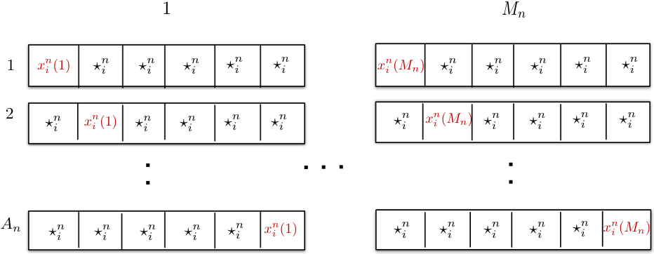
Refer to caption
Fig. 3: Extended codebook.
Proof:

User i∈[Kn]i\in[{K_{n}}] has a codebook with Mn=en​RM_{n}=e^{nR} codewords of length nn. Define for i∈[Kn]i\in[{K_{n}}] an ‘extended codebook’ consisting of An​MnA_{n}M_{n} codewords of length n​AnnA_{n} constructed such that ∀m∈[Mn]\forall m\in[M_{n}] and ∀ti∈[An]\forall t_{i}\in[A_{n}]

X~in​An(mi,ti):=[⋆in⁡(ti−1)fi(mi)⋆in⁡(An−ti)],\displaystyle\widetilde{X}_{i}^{nA_{n}}(m_{i},t_{i}):=\big[\star_{i}^{n(t_{i}-1)}\,f_{i}(m_{i})\,\star_{i}^{n(A_{n}-t_{i})}\big],

as depicted in Fig. 3. By using Fanno’s inequality, i.e., H⁡(X1n​An,…,XKnn​An|Yn​An)≤n​ϵn:ϵn→0H({X}_{1}^{nA_{n}},\ldots,{X}_{K_{n}}^{nA_{n}}|Y^{nA_{n}})\leq n\epsilon_{n}:\epsilon_{n}\to 0 as n→∞n\to\infty, for any codebook of length n​AnnA_{n} we have

H⁡(X1n​An,…,XKnn​An)=H⁡(m1,t1,…,mKn,tKn)\displaystyle H({X}_{1}^{nA_{n}},\ldots,{X}_{K_{n}}^{nA_{n}})=H(m_{1},t_{1},\ldots,m_{K_{n}},t_{K_{n}})
=n​Kn​(α+R)\displaystyle=nK_{n}\left(\alpha+R\right)
=H⁡(X1n​An,…,XKnn​An|Yn​An)+I⁡(X1n​An,…,XKnn​An,Yn​An)\displaystyle=H({X}_{1}^{nA_{n}},\ldots,{X}_{K_{n}}^{nA_{n}}|Y^{nA_{n}})+I({X}_{1}^{nA_{n}},\ldots,{X}_{K_{n}}^{nA_{n}};Y^{nA_{n}})
≤nϵn+nen​α|𝒴|⟺\displaystyle\leq n\epsilon_{n}+ne^{n\alpha}\ |\mathcal{Y}|\quad\Longleftrightarrow
ν+log⁡(1+1α​Kn​∑i∈[Kn]Ri)n≤α+log⁡(1+ϵnen​α​∣𝒴∣)n,\displaystyle\nu+\frac{\log\left(1+\frac{1}{\alpha K_{n}}\sum_{i\in[K_{n}]}R_{i}\right)}{n}\leq\alpha+\frac{\log\left(1+\frac{\epsilon_{n}}{e^{n\alpha}\mid\mathcal{Y}\mid}\right)}{n},

where log⁡(1+1α​Kn​∑i∈[Kn]Ri)n≥0\frac{\log\left(1+\frac{1}{\alpha K_{n}}\sum_{i\in[K_{n}]}R_{i}\right)}{n}\geq 0 and log⁡(1+ϵnen​α​∣𝒴∣)n≥0\frac{\log(1+\frac{\epsilon_{n}}{e^{n\alpha}\mid\mathcal{Y}\mid})}{n}\geq 0 vanish as nn goes to infinity. This implies that ν≤α\nu\leq\alpha is a necessary condition for reliable communications. In other words, for ν>α\nu>\alpha not even synchronization (i.e., Mn=1,∀i∈[Kn]M_{n}=1,\forall i\in[K_{n}]) is possible. ∎

V Discussion and Conclusion

In this paper we studied a Strongly Asynchronous and Slotted Massive Access Channel (SAS-MAC) where Kn:=en​νK_{n}:=e^{n\nu} different users transmit a randomly selected message among Mn:=en​RM_{n}:=e^{nR} ones within a strong asynchronous window of length An:=en​αA_{n}:=e^{n\alpha} blocks of nn channel uses each. We found inner and outer bounds on the (R,α,ν)(R,\alpha,\nu) tuples. Our analysis is based on a global probability of error in which we required all users messages and identities to be jointly correctly decoded. Our results are focused on the region ν<α2\nu<\frac{\alpha}{2}, where the probability of user collisions in vanishing. We proved in Theorem 6 that for the region ν>α\nu>\alpha, not even synchronization is possible. Hence, we would like to take this chance to discuss some of the difficulties that one may face in analyzing the region α2≤ν≤α\frac{\alpha}{2}\leq\nu\leq\alpha.

As we have mentioned before, for the region ν<α2\nu<\frac{\alpha}{2}, with probability (AnKn)(An)Kn\frac{\binom{A_{n}}{K_{n}}}{(A_{n})^{K_{n}}} which approaches to one as blocklength nn goes to infinity, the users transmit in distinct blocks. Hence, in analyzing the probability of error of our achievable schemes, we could safely condition on the hypothesis that users are not colliding. For the region α2≤ν≤α\frac{\alpha}{2}\leq\nu\leq\alpha, we lose this simplifying assumption. In particular, based on Lemma 2 (proved in the Appendix -F), for the region α2≤ν≤α\frac{\alpha}{2}\leq\nu\leq\alpha, the probability of every arrangement of users is itself vanishing in the blocklength.

Lemma 2.

For the region α2≤ν≤α\frac{\alpha}{2}\leq\nu\leq\alpha the non-colliding arrangement of users has the highest probability among all possible arrangements, yet, the probability of this event is also vanishing as blocklength nn goes to infinity.

As a consequence of Lemma 2, one needs to propose an achievable scheme that accounts for every possible arrangement and collision of users and drives the probability of error in all (or most) of the hypothesis to zero. It is also worth noting that the number of possible hypotheses is doubly exponential in the blocklength. Finally, it is worth emphasizing the reason why the authors in [15] can get to ν≤α\nu\leq\alpha. In [15] the authors require the recovery of the messages of a large fraction of users and they also require the per-user probability of error to be vanishing. To prove whether or not strictly positive (R,α,ν)(R,\alpha,\nu) are possible in the region α2≤ν≤α\frac{\alpha}{2}\leq\nu\leq\alpha, with vanishing global probability of error, is an open problem.

-A Proof of Lemma 1

We first consider the case that r is an even number and then prove

r​(nk)r2−1​(G⁡(c1)+…​G​(cNr,k))≤Nr,k​rnk​(a12+…+ank2)r2.\displaystyle r\!\left(n_{k}\right)^{\frac{r}{2}-1}\left(G(c_{1})+\ldots G(c_{N_{r,k}})\right)\!\leq\!\frac{N_{r,k}r}{n_{k}}\!\left(a_{1}^{2}+\ldots+{a_{n_{k}}}^{2}\right)^{\frac{r}{2}}\!. (85)

We may drop the subscripts and use N:=Nr,kN:=N_{r,k} and n:=nkn:=n_{k} in the following for notational ease. Our goal is to expand the right hand side (RHS) of (85) such that all elements have coefficient 11. Then, we parse these elements into NN different groups (details will be provided later) such that using the AM-GM inequality (i.e., n​(∏i=1nai)1n≤∑i=1nain\left(\prod_{i=1}^{n}a_{i}\right)^{\frac{1}{n}}\leq\sum_{i=1}^{n}a_{i}) on each group, we get one of the NN terms on the LHS of (85). Before stating the rigorous proof, we provide an example of this strategy for the graph with k=4k=4 vertices shown in Fig. 4. In this example, we consider the Lemma for r=4r=4 cycles (for which N=3N=3).

Fig. 4: A complete graph with 44 vertices

We may expand the RHS in (85) as

2​(a12+…+a62)2=Θ1+Θ2+Θ3,\displaystyle\qquad 2\left(a_{1}^{2}+\ldots+a_{6}^{2}\right)^{2}=\Theta_{1}+\Theta_{2}+\Theta_{3},
Θ1={a14+a24+a34+a44+a12a32+a12a32+a22a42+a22a42\displaystyle\Theta_{1}\!=\!\big\{a_{1}^{4}+a_{2}^{4}+a_{3}^{4}+a_{4}^{4}+a_{1}^{2}a_{3}^{2}+a_{1}^{2}a_{3}^{2}+a_{2}^{2}a_{4}^{2}+a_{2}^{2}a_{4}^{2}
+a12​a22+a12​a22+a12​a22+a12​a22+a12​a42+a12​a42+a12​a42+a12​a42\displaystyle+a_{1}^{2}a_{2}^{2}+a_{1}^{2}a_{2}^{2}+a_{1}^{2}a_{2}^{2}+a_{1}^{2}a_{2}^{2}+a_{1}^{2}a_{4}^{2}+a_{1}^{2}a_{4}^{2}+a_{1}^{2}a_{4}^{2}+a_{1}^{2}a_{4}^{2}
+a22a32+a22a32+a22a32+a22a32+a32a42+a32a42+a32a42+a32a42}\displaystyle+a_{2}^{2}a_{3}^{2}+a_{2}^{2}a_{3}^{2}+a_{2}^{2}a_{3}^{2}+a_{2}^{2}a_{3}^{2}+a_{3}^{2}a_{4}^{2}+a_{3}^{2}a_{4}^{2}+a_{3}^{2}a_{4}^{2}+a_{3}^{2}a_{4}^{2}\big\}
Θ2={a14+a64+a34+a54+a52a62+a52a62+a12a32+a12a32\displaystyle\Theta_{2}\!=\!\big\{a_{1}^{4}+a_{6}^{4}+a_{3}^{4}+a_{5}^{4}+a_{5}^{2}a_{6}^{2}+a_{5}^{2}a_{6}^{2}+a_{1}^{2}a_{3}^{2}+a_{1}^{2}a_{3}^{2}
+a12​a62+a12​a62+a12​a62+a12​a62+a12​a52+a12​a52+a12​a52+a12​a52\displaystyle+a_{1}^{2}a_{6}^{2}+a_{1}^{2}a_{6}^{2}+a_{1}^{2}a_{6}^{2}+a_{1}^{2}a_{6}^{2}+a_{1}^{2}a_{5}^{2}+a_{1}^{2}a_{5}^{2}+a_{1}^{2}a_{5}^{2}+a_{1}^{2}a_{5}^{2}
+a32a62+a32a62+a32a62+a32a62+a32a52+a32a52+a32a52+a32a52}\displaystyle+a_{3}^{2}a_{6}^{2}+a_{3}^{2}a_{6}^{2}+a_{3}^{2}a_{6}^{2}+a_{3}^{2}a_{6}^{2}+a_{3}^{2}a_{5}^{2}+a_{3}^{2}a_{5}^{2}+a_{3}^{2}a_{5}^{2}+a_{3}^{2}a_{5}^{2}\big\}
Θ3={a44+a54+a24+a64+a52a62+a52a62+a22a42+a22a42\displaystyle\Theta_{3}\!=\!\big\{a_{4}^{4}+a_{5}^{4}+a_{2}^{4}+a_{6}^{4}+a_{5}^{2}a_{6}^{2}+a_{5}^{2}a_{6}^{2}+a_{2}^{2}a_{4}^{2}+a_{2}^{2}a_{4}^{2}
+a42​a52+a42​a52+a42​a52+a42​a52+a42​a62+a42​a62+a42​a62+a42​a62\displaystyle+a_{4}^{2}a_{5}^{2}+a_{4}^{2}a_{5}^{2}+a_{4}^{2}a_{5}^{2}+a_{4}^{2}a_{5}^{2}+a_{4}^{2}a_{6}^{2}+a_{4}^{2}a_{6}^{2}+a_{4}^{2}a_{6}^{2}+a_{4}^{2}a_{6}^{2}
+a22a52+a22a52+a22a52+a22a52+a22a62+a22a62+a22a62+a22a62}.\displaystyle+a_{2}^{2}a_{5}^{2}+a_{2}^{2}a_{5}^{2}+a_{2}^{2}a_{5}^{2}+a_{2}^{2}a_{5}^{2}+a_{2}^{2}a_{6}^{2}+a_{2}^{2}a_{6}^{2}+a_{2}^{2}a_{6}^{2}+a_{2}^{2}a_{6}^{2}\big\}.

It can be easily seen that if we use the AM-GM inequality on Θ1\Theta_{1}, Θ2\Theta_{2} and Θ3\Theta_{3}, we can get the lower bound equal to 24​(a1​a2​a3​a4),24​(a1​a6​a3​a5)24(a_{1}a_{2}a_{3}a_{4}),24(a_{1}a_{6}a_{3}a_{5}) and 24​(a4​a5​a2​a6)24(a_{4}a_{5}a_{2}a_{6}), respectively where r​nr2−1=24rn^{\frac{r}{2}-1}=24 and hence (85) holds in this example.

We proceed to prove Lemma 1 for arbitrary kk and (even) r≥2r\geq 2. We propose the following scheme to group the elements on the RHS of (85) and then we prove that this grouping indeed leads to the claimed inequality in the Lemma.

Grouping scheme

For each cycle ci={ai1​…,air}c_{i}=\{a_{i_{1}}\ldots,a_{i_{r}}\}, we need a group of elements, Θi\Theta_{i}, from the RHS of (85). In this regard, we consider all possible subsets of the edges of cycle cic_{i} with 1:r21:\frac{r}{2} elements (e.g. {{ai1},…​{ai1,ai2},…​{ai1​…,air/2},…}\left\{\{a_{i_{1}}\},\ldots\{a_{i_{1}},a_{i_{2}}\},\ldots\{a_{i_{1}}\ldots,a_{i_{r/2}}\},\ldots\right\}). For each one of these subsets, we find the respective elements from the RHS of (85) that is the multiplication of the elements in that subset. For example, for the subset {ai1,ai2,ai3}\{a_{i_{1}},a_{i_{2}},a_{i_{3}}\}, we consider the elements like ai1ni1​ai2ni2​ai3ni3a_{i_{1}}^{n_{i_{1}}}a_{i_{2}}^{n_{i_{2}}}a_{i_{3}}^{n_{i_{3}}} for all possible ni1,ni2,ni3>0n_{i_{1}},n_{i_{2}},n_{i_{3}}>0 from the RHS of (85). However, note that we do not assign all such elements to cycle cic_{i} only. If there are ll cycles of length rr that all contain {ai1,ai2,ai3}\{a_{i_{1}},a_{i_{2}},a_{i_{3}}\}, we should assign 1l\frac{1}{l} of the elements like ai1ni1​ai2ni2​ai3ni3,ni1,ni2,ni3>0a_{i_{1}}^{n_{i_{1}}}a_{i_{2}}^{n_{i_{2}}}a_{i_{3}}^{n_{i_{3}}},\ n_{i_{1}},n_{i_{2}},n_{i_{3}}>0 to cycle cic_{i} (so that we can assign the same amount of elements to other cycles with similar edges).

We state some facts, which can be easily verified:

Fact 1. In a complete graph KkK_{k}, there are N=Nr,k=(kr)​(r−1)!2N=N_{r,k}=\binom{k}{r}\frac{(r-1)!}{2} cycles of length rr.

Fact 2. By expanding the RHS of (85) such that all elements have coefficient 11, we end up with (N​rn)​nr2\left(\frac{Nr}{n}\right)n^{\frac{r}{2}} elements.

Fact 3. Expanding the RHS of (85) such that all elements have coefficient 11, and finding their product yields

(a1×…×an)(N​rn)​r​nr2−1.\left(a_{1}\times\ldots\times a_{n}\right)^{\left(\frac{Nr}{n}\right)rn^{\frac{r}{2}-1}}.

Fact 4. In above grouping scheme each element on the RHS of (85) is summed in exactly one group. Hence, by symmetry and Fact 2, each group is the sum of r​nr2−1rn^{\frac{r}{2}-1} elements.

Now, consider any two cycles ci(e)={ai1,…,air},cj(e)={aj1,…,ajr}c^{(e)}_{i}=\{a_{i_{1}},\ldots,a_{i_{r}}\},c^{(e)}_{j}=\{a_{j_{1}},\ldots,a_{j_{r}}\}. Assume that using the above grouping scheme, we get the group of elements Θi,Θj\Theta_{i},\Theta_{j} (where by fact 3 each one is the sum of r​nr2−1rn^{\frac{r}{2}-1} elements). If we apply the AM-GM inequality on each one of the two groups, we get

Θi≥r​nr2−1​(ai1ni1×…×airn1r)(1r​nr2−1),\displaystyle\Theta_{i}\geq rn^{\frac{r}{2}-1}\left(a_{i_{1}}^{n_{i_{1}}}\times\ldots\times a_{i_{r}}^{n_{1_{r}}}\right)^{\left(\frac{1}{rn^{\frac{r}{2}-1}}\right)},
Θj≥r​nr2−1​(aj1nj1×…×ajrnjr)(1r​nr2−1),\displaystyle\Theta_{j}\geq rn^{\frac{r}{2}-1}\left(a_{j_{1}}^{n_{j_{1}}}\times\ldots\times a_{j_{r}}^{n_{j_{r}}}\right)^{\left(\frac{1}{rn^{\frac{r}{2}-1}}\right)},

where ∏t=1raitnit\prod_{t=1}^{r}a_{i_{t}}^{n_{i_{t}}} is the product of the elements in Θi\Theta_{i}. By symmetry of the grouping scheme for different cycles, it is obvious that ∀t∈[r],nit=njt\forall t\in[r],n_{i_{t}}=n_{j_{t}}. Hence nit=njt=pt,∀i,j∈[N]n_{i_{t}}=n_{j_{t}}=p_{t},\forall i,j\in[N]. i.e., we have

Θi\displaystyle\Theta_{i} ≥r​nr2−1​(ai1p1×…×airpr)(1r​nr2−1).\displaystyle\geq rn^{\frac{r}{2}-1}\left(a_{i_{1}}^{p_{1}}\times\ldots\times a_{i_{r}}^{p_{r}}\right)^{\left(\frac{1}{rn^{\frac{r}{2}-1}}\right)}. (86)

By symmetry of the grouping scheme over the elements of each cycle, we also get that nik=nil=qi,∀k,l∈[r]n_{i_{k}}=n_{i_{l}}=q_{i},\forall k,l\in[r]. i.e.

Θi≥r​nr2−1​(ai1qi×…×airqi)(1r​nr2−1).\displaystyle\Theta_{i}\geq rn^{\frac{r}{2}-1}\left(a_{i_{1}}^{q_{i}}\times\ldots\times a_{i_{r}}^{q_{i}}\right)^{\left(\frac{1}{rn^{\frac{r}{2}-1}}\right)}. (87)

It can be seen from (86) and (87) that all the elements of all groups have the same power nit=p,∀i∈[N],t∈[r]n_{i_{t}}=p,\forall i\in[N],t\in[r]. i.e.,

Θi\displaystyle\Theta_{i} ≥r​nr2−1​(ai1p×…×airp)(1r​nr2−1).\displaystyle\geq rn^{\frac{r}{2}-1}\left(a_{i_{1}}^{p}\times\ldots\times a_{i_{r}}^{p}\right)^{\left(\frac{1}{rn^{\frac{r}{2}-1}}\right)}.

Since each element on the RHS of (85) is assigned to one and only one group and since ∏t=1raitnit=∏t=1raitp\prod_{t=1}^{r}a_{i_{t}}^{n_{i_{t}}}=\prod_{t=1}^{r}a_{i_{t}}^{p} is the product of the elements of each group Θi\Theta_{i}, the product of all elements in Θ1+…+ΘN\Theta_{1}+\ldots+\Theta_{N} (which is equal to product of the elements in the expanded version of the RHS of (85)) is ∏i=1N∏t=1raitp\prod_{i=1}^{N}\prod_{t=1}^{r}a_{i_{t}}^{p}.

In addition, since each aia_{i} appears in exactly N​rn\frac{Nr}{n} of the cycles, by Fact 3 and a double counting argument, we have

p×N​rn=(N​rn)​r​nr2−1,p\times\frac{Nr}{n}=\left(\frac{Nr}{n}\right)rn^{\frac{r}{2}-1},

and hence p=r​nr2−1p=rn^{\frac{r}{2}-1}. Hence, the lower bound of the AM-GM inequality on the Θ1+…+ΘN\Theta_{1}+\ldots+\Theta_{N}, will result in

r​nr2−1​G​(c1)+…+r​nr2−1​G​(cNr),rn^{\frac{r}{2}-1}G(c_{1})+\ldots+rn^{\frac{r}{2}-1}G(c_{N_{r}}),

and the Lemma is proved for even rr.

For odd values of rr, the problem that may arise by using the grouping strategy in its current form, is when r<k2r<\frac{k}{2}. In this case, some of the terms on the RHS of (85) may contain multiplication of aia_{i}’s that are not present in any of the G⁡(ci)G(c_{i})’s. To overcome this, take both sides to the power of 2​m2m for the smallest mm such that r​m>k2rm>\frac{k}{2}. Then the RHS of (85) is at most the multiplication of r​mrm different aia_{i}’s and on the LHS of (85), there are 2​m2m cycles of length rr multiplied together. By our choice of 2​m2m, now, all possible combinations of aia_{i}’s on the RHS are present in at least one cycle multiplication in the LHS. Hence, it is straightforward to use the same strategy as even values of rr to prove the theorem for the odd values of rr.

-B Proof of (9)

By Lemma 1 and (6) we can write

Pe(n)\displaystyle P_{e}^{(n)} ≤∑r=2An∑c∈CAn(r)G⁡(c)\displaystyle\leq\sum_{r=2}^{A_{n}}\sum_{c\in C_{A_{n}}^{(r)}}G(c)
≤∑r=2AnNr,An(nAn)r2​(a12+…+anAn2)r/2\displaystyle\leq\sum_{r=2}^{A_{n}}\frac{N_{r,A_{n}}}{\left({n_{A_{n}}}\right)^{\frac{r}{2}}}\left(a_{1}^{2}+\ldots+a_{n_{A_{n}}}^{2}\right)^{r/2}
≤∑r=2An4r​(∑1≤i<j≤Ane−2​n​B​(Pi,Pj))r/2\displaystyle\leq\sum_{r=2}^{A_{n}}4^{r}\left(\sum_{\begin{subarray}{c}1\leq i<j\leq A_{n}\end{subarray}}e^{-2nB(P_{i},P_{j})}\right)^{r/2} (88)
≤16​(∑1≤i<j≤Ane−2​n​B​(Pi,Pj))1−4​∑1≤i<j≤Ane−2​n​B​(Pi,Pj),\displaystyle\leq\frac{16\left(\sum_{\begin{subarray}{c}1\leq i<j\leq A_{n}\end{subarray}}e^{-2nB(P_{i},P_{j})}\right)}{1-4\sqrt{\sum_{\begin{subarray}{c}1\leq i<j\leq A_{n}\end{subarray}}e^{-2nB(P_{i},P_{j})}}}, (89)

where (88) is by Fact 1 (see Appendix -A) and

Nr,An(nAn)r/2=(Anr)⁡(r−1)!/2((An2))r/2≤4r.\frac{N_{r,A_{n}}}{\left({n_{A_{n}}}\right)^{r/2}}=\frac{\binom{A_{n}}{r}(r-1)!/2}{\left(\binom{A_{n}}{2}\right)^{r/2}}\leq 4^{r}.

As the result, (89) will go to zero as nn goes to infinity if

limn→∞∑1≤i<j≤Ane−2​n​B​(Pi,Pj)=0.\lim_{n\to\infty}\sum_{\begin{subarray}{c}1\leq i<j\leq A_{n}\end{subarray}}e^{-2nB(P_{i},P_{j})}=0.

-C Proof of (12)

We upper bound the denominator of (10) by

ℙ[ξi,j,ξi,k]=ℙ[logPi​(Xjn)Pj​(Xjn)+logPj​(Xin)Pi​(Xin)≥0∩logPi​(Xkn)Pk​(Xkn)+logPk​(Xin)Pi​(Xin)≥0]\displaystyle\!\mathbb{P}[\xi_{i,j},\xi_{i,k}]=\mathbb{P}\left[\log\frac{P_{i}(X^{n}_{j})}{P_{j}(X^{n}_{j})}+\log\frac{P_{j}(X_{i}^{n})}{P_{i}(X_{i}^{n})}\geq 0\cap\ \log\frac{P_{i}(X^{n}_{k})}{P_{k}(X^{n}_{k})}+\log\frac{P_{k}(X_{i}^{n})}{P_{i}(X_{i}^{n})}\geq 0\right]
≤ℙ[logPi​(Xjn)Pj​(Xjn)+logPj​(Xin)Pi​(Xin)+logPi​(Xkn)Pk​(Xkn)+logPk​(Xin)Pi​(Xin)≥0]\displaystyle\leq\mathbb{P}\left[\log\frac{P_{i}(X^{n}_{j})}{P_{j}(X^{n}_{j})}+\log\frac{P_{j}(X_{i}^{n})}{P_{i}(X_{i}^{n})}+\log\frac{P_{i}(X^{n}_{k})}{P_{k}(X^{n}_{k})}+\log\frac{P_{k}(X_{i}^{n})}{P_{i}(X_{i}^{n})}\geq 0\right]
≤exp⁡{n​inftlog⁡(𝔼⁡[(Pi​(Xjn)Pj​(Xjn)⋅Pj​(Xin)Pi​(Xin)⋅Pi​(Xkn)Pk​(Xkn)⋅Pk​(Xin)Pi​(Xin))t])}\displaystyle\leq\exp\Bigg\{n\inf_{t}\log\left(\mathbb{E}\left[\left(\!\frac{P_{i}(X^{n}_{j})}{P_{j}(X^{n}_{j})}\cdot\frac{P_{j}(X_{i}^{n})}{P_{i}(X_{i}^{n})}\cdot\frac{P_{i}(X^{n}_{k})}{P_{k}(X^{n}_{k})}\cdot\frac{P_{k}(X_{i}^{n})}{P_{i}(X_{i}^{n})}\right)^{t}\right]\right)\Bigg\}
≤exp⁡{n​log⁡𝔼⁡[(Pi​(Xjn)Pj​(Xjn)⋅Pj​(Xin)Pi​(Xin)⋅Pi​(Xkn)Pk​(Xkn)⋅Pk​(Xin)Pi​(Xin))12]}\displaystyle\!\!\leq\!\exp\left\{\!n\log\mathbb{E}\left[\!\left(\frac{P_{i}(X^{n}_{j})}{P_{j}(X^{n}_{j})}\!\cdot\!\frac{P_{j}(X_{i}^{n})}{P_{i}(X_{i}^{n})}\cdot\!\frac{P_{i}(X^{n}_{k})}{P_{k}(X^{n}_{k})}\cdot\!\frac{P_{k}(X_{i}^{n})}{P_{i}(X_{i}^{n})}\!\right)^{\frac{1}{2}}\!\right]\right\}
=exp⁡{−n​B​(Pi,Pj)−n​B​(Pj,Pk)−n​B​(Pi,Pk)}.\displaystyle=\exp\left\{-nB({P_{i}},{P_{j}})-nB({P_{j}},P_{k})-nB({P_{i}},{P_{k}})\right\}. (90)

An upper bound for ℙ⁡[ξi,j,ξk,l]\mathbb{P}\left[\xi_{i,j},\xi_{k,l}\right] can be derived similarly.

-D Proof of (59b)

We find an upper bound on C(.,Q⋆,Pi,Qi)C(\,.\,,Q_{\star},P_{i},Q_{i}) by noting that μ0,i​(t)\mu_{0,i}(t) defined in (57) is concave in tt with μ0,i​(1)=0\mu_{0,i}(1)=0 and

∂μ0,i​(t)∂t∣t=1=−I(Pi,Qi)−D([PiQi]∥Q⋆)≤0.\displaystyle\frac{\partial\mu_{0,i}(t)}{\partial t}\mid_{t=1}=-I(P_{i},Q_{i})-D([P_{i}Q_{i}]\parallel Q_{\star})\leq 0.

Hence μ0,i​(t)\mu_{0,i}(t) is always less than (I(Pi,Qi)+D([PiQi]∥Q⋆))(1−t)(I(P_{i},Q_{i})+D([P_{i}Q_{i}]\parallel Q_{\star}))(1-t) and that for 0≤t≤10\leq t\leq 1 it is always less than I(Pi,Qi)+D([PiQi]∥Q⋆)I(P_{i},Q_{i})+D([P_{i}Q_{i}]\parallel Q_{\star}). The inequality in (59c) follows similarly.

-E Proof of (73) and (74)

Before deriving lower bounds on (73) and (74), we note that by the Type-counting Lemma [16], at the expense of a small decrease in the rate (which vanishes in the limit for large blocklength) we may restrict our attention to constant composition codewords. Henceforth, we assume that the composition of the codewords for user i∈[Kn]i\in[K_{n}] is given by PiP_{i}. Moreover, to make this paper self-contained, we restate the following Lemmas that we use in the rest of the proof.

Lemma 3 (Compensation Identity).

For arbitrary πi:∑i=1Kπi=1\pi_{i}:\sum_{i=1}^{K}\pi_{i}=1 and arbitrary probability distribution functions Pi∈𝒫𝒳,i∈[K]P_{i}\in\mathcal{P}_{\mathcal{X}},i\in[K], we define P¯​(x)=∑i=1Kπi​Pi​(x)\bar{P}(x)=\sum_{i=1}^{K}\pi_{i}P_{i}(x). Then for any probability distribution function RR we have:

D(P¯∥R)+∑i=1KπiD(Pi∥P¯)=∑i=1KπiD(Pi||R).\displaystyle D\left(\bar{P}\parallel R\right)+\sum_{i=1}^{K}\pi_{i}D\left(P_{i}\parallel\bar{P}\right)=\sum_{i=1}^{K}\pi_{i}D(P_{i}||R). (91)
Lemma 4 (Fano).

Let FF be an arbitrary set of size NN. For P¯=∑θ∈FPθN\bar{P}=\frac{\sum_{\theta\in F}P_{\theta}}{N} we have

1N∑θ∈FD(Pθ∥P¯)≥(1−r¯)log(N(1−r¯))+r¯log(N​r¯N−1),\displaystyle\frac{1}{N}\sum_{\theta\in F}D\left(P_{\theta}\parallel\bar{P}\right)\geq\left(1-\bar{r}\right)\log\left(N(1-\bar{r})\right)+\bar{r}\log\left(\frac{N\bar{r}}{N-1}\right), (92)

where

r¯:=infT1N∑θ∈FPθ{T≠θ}\displaystyle\bar{r}:=\inf_{T}\frac{1}{N}\sum_{\theta\in F}P_{\theta}\left\{T\neq\theta\right\} (93)

in which the infimum is taken over all possible estimators TT.

We now continue with the proof of (73). Using the Chernoff bound we can write

Q⋆n\displaystyle Q_{\star}^{n} [logPYn¯Q⋆n(Yn)≥1Fn∑i=1Kn∑m=1MnD(Qi,mnλi∥Q⋆n)−D(Qi,mnλi∥PYn¯)]≐Chernoffe−suptA(t).\displaystyle\left[\log\frac{\widebar{P_{Y^{n}}}}{Q_{\star}^{n}}(Y^{n})\geq\frac{1}{F_{n}}\sum_{i=1}^{K_{n}}\sum_{m=1}^{M_{n}}D\left({Q_{i,m}^{n}}_{\lambda_{i}}\parallel Q_{\star}^{n}\right)-D\left({Q_{i,m}^{n}}_{\lambda_{i}}\parallel\widebar{P_{Y^{n}}}\right)\right]\overset{\text{Chernoff}}{\doteq}e^{-\sup_{t}A(t)}. (94)

The Chernoff bound exponent, suptA⁡(t)\sup_{t}A(t), is expressed and simplified as follows

A⁡(t)\displaystyle A(t) :=tFn∑i=1Kn∑m=1MnD(Qi,mnλi∥Q⋆n)−D(Qi,mnλi∥PYn¯)−log𝔼Q⋆n[(PYn¯Q⋆n(Yn))t]\displaystyle:=\frac{t}{F_{n}}\sum_{i=1}^{K_{n}}\sum_{m=1}^{M_{n}}D\left({Q_{i,m}^{n}}_{\lambda_{i}}\parallel Q_{\star}^{n}\right)-D\left({Q_{i,m}^{n}}_{\lambda_{i}}\parallel\widebar{P_{Y^{n}}}\right)-\log\mathbb{E}_{Q_{\star}^{n}}\left[\left(\frac{\widebar{P_{Y^{n}}}}{Q_{\star}^{n}}(Y^{n})\right)^{t}\right]
=tFn∑i=1Kn∑m=1Mn∑ynQi,mnλi(yn)logPYn¯​(yn)Q⋆n​(yn)−log∑yn(PYn¯(yn))t(Q⋆n(yn))1−t\displaystyle=\frac{t}{F_{n}}\sum_{i=1}^{K_{n}}\sum_{m=1}^{M_{n}}\sum_{y^{n}}{Q_{i,m}^{n}}_{\lambda_{i}}(y^{n})\log\frac{\widebar{P_{Y^{n}}}(y^{n})}{Q_{\star}^{n}(y^{n})}-\log\sum_{y^{n}}\left(\widebar{P_{Y^{n}}}(y^{n})\right)^{t}\left(Q_{\star}^{n}(y^{n})\right)^{1-t}
=1Fn​∑i=1Kn∑m=1Mn∑ynQi,mnλi​(yn)​log⁡(PYn¯​(yn))t​(Q⋆n​(yn))1−t∑yn(PYn¯​(yn))t​(Q⋆n​(yn))1−tQ⋆n​(yn)\displaystyle=\frac{1}{F_{n}}\sum_{i=1}^{K_{n}}\sum_{m=1}^{M_{n}}\sum_{y^{n}}{Q_{i,m}^{n}}_{\lambda_{i}}(y^{n})\log\frac{\frac{\left(\widebar{P_{Y^{n}}}(y^{n})\right)^{t}\left(Q_{\star}^{n}(y^{n})\right)^{1-t}}{\sum_{y^{n}}\left(\widebar{P_{Y^{n}}}(y^{n})\right)^{t}\left(Q_{\star}^{n}(y^{n})\right)^{1-t}}}{Q_{\star}^{n}(y^{n})}
=1Fn​∑i=1Kn∑m=1Mn∑ynQi,mnλi​(yn)​log⁡(PYn¯)t​(yn)Q⋆n​(yn)\displaystyle=\frac{1}{F_{n}}\sum_{i=1}^{K_{n}}\sum_{m=1}^{M_{n}}\sum_{y^{n}}{Q_{i,m}^{n}}_{\lambda_{i}}(y^{n})\log\frac{\left(\widebar{P_{Y^{n}}}\right)_{t}(y^{n})}{Q_{\star}^{n}(y^{n})}
=1Fn∑i=1Kn∑m=1MnD(Qi,mnλi∥Q⋆n)−D(Qi,mnλi∥(PYn¯)t)\displaystyle=\frac{1}{F_{n}}\sum_{i=1}^{K_{n}}\sum_{m=1}^{M_{n}}D\left({Q_{i,m}^{n}}_{\lambda_{i}}\parallel Q_{\star}^{n}\right)-D\left({Q_{i,m}^{n}}_{\lambda_{i}}\parallel\left(\widebar{P_{Y^{n}}}\right)_{t}\right)
=1Kn∑i=1KnnD(Qiλi∥Q⋆|Pi)−1Fn∑i=1Kn∑m=1MnD(Qi,mnλi∥(PYn¯)t),\displaystyle=\frac{1}{K_{n}}\sum_{i=1}^{K_{n}}nD\left({Q_{i}}_{\lambda_{i}}\parallel Q_{\star}|P_{i}\right)-\frac{1}{F_{n}}\sum_{i=1}^{K_{n}}\sum_{m=1}^{M_{n}}D\left({Q_{i,m}^{n}}_{\lambda_{i}}\parallel\left(\widebar{P_{Y^{n}}}\right)_{t}\right), (95)

where (95) is the result of constant composition structure of the codewords. As a result,

suptA(t)=1Kn∑i=1KnnD(Qiλi∥Q⋆|Pi)−inft{1Fn∑i=1FnD(Qi,mnλi∥(PYn¯)t)}.\displaystyle\sup_{t}A(t)=\frac{1}{K_{n}}\sum_{i=1}^{K_{n}}nD\left({Q_{i}}_{\lambda_{i}}\parallel Q_{\star}|P_{i}\right)-\inf_{t}\left\{\frac{1}{F_{n}}\sum_{i=1}^{F_{n}}D\left({Q_{i,m}^{n}}_{\lambda_{i}}\parallel\left(\widebar{P_{Y^{n}}}\right)_{t}\right)\right\}. (96)

Moreover,

inft1Fn∑i=1Kn∑m=1MnD(Qi,mnλi∥(PYn¯)t)\displaystyle\inf_{t}\frac{1}{F_{n}}\sum_{i=1}^{K_{n}}\sum_{m=1}^{M_{n}}D\left({Q_{i,m}^{n}}_{\lambda_{i}}\parallel\left(\widebar{P_{Y^{n}}}\right)_{t}\right) (97)
=inft1Fn​∑i=1Kn∑m=1Mn∑ynQi,mnλi​(yn)​log⁡Qi,mnλi​(yn)(PYn¯)t​(yn)\displaystyle=\inf_{t}\frac{1}{F_{n}}\sum_{i=1}^{K_{n}}\sum_{m=1}^{M_{n}}\sum_{y^{n}}{Q_{i,m}^{n}}_{\lambda_{i}}(y^{n})\log\frac{{Q_{i,m}^{n}}_{\lambda_{i}}(y^{n})}{\left(\widebar{P_{Y^{n}}}\right)_{t}(y^{n})} (98)
=inft1Fn​∑i=1Kn∑m=1Mn∑ynQi,mnλi​(yn)​log⁡Qi,mnλi​(yn)(PYn¯)t​(yn)⋅PYn(λ)¯​(yn)PYn(λ)¯​(yn)\displaystyle=\inf_{t}\frac{1}{F_{n}}\sum_{i=1}^{K_{n}}\sum_{m=1}^{M_{n}}\sum_{y^{n}}{Q_{i,m}^{n}}_{\lambda_{i}}(y^{n})\log\frac{{Q_{i,m}^{n}}_{\lambda_{i}}(y^{n})}{\left(\widebar{P_{Y^{n}}}\right)_{t}(y^{n})}\cdot\frac{{\widebar{P_{Y^{n}}^{(\lambda)}}}(y^{n})}{\widebar{P_{Y^{n}}^{(\lambda)}}(y^{n})} (99)
=inft1Fn∑i=1Kn∑m=1MnD(Qi,mnλi∥PYn(λ)¯)+D(PYn(λ)¯∥(PYn¯)t)\displaystyle=\inf_{t}\frac{1}{F_{n}}\sum_{i=1}^{K_{n}}\sum_{m=1}^{M_{n}}D\left({Q_{i,m}^{n}}_{\lambda_{i}}\parallel\widebar{P_{Y^{n}}^{(\lambda)}}\right)+D\left(\widebar{P_{Y^{n}}^{(\lambda)}}\parallel\left(\widebar{P_{Y^{n}}}\right)_{t}\right) (100)
≥1Fn∑i=1Kn∑m=1MnD(Qi,mnλi∥PYn(λ)¯).\displaystyle\geq\frac{1}{F_{n}}\sum_{i=1}^{K_{n}}\sum_{m=1}^{M_{n}}D\left({Q_{i,m}^{n}}_{\lambda_{i}}\parallel\widebar{P_{Y^{n}}^{(\lambda)}}\right). (101)

Note that PYn(λ)¯\widebar{P_{Y^{n}}^{(\lambda)}} is the average of Qi,mnλi{Q_{i,m}^{n}}_{\lambda_{i}} over m,im,i’s (m∈[Mn],i∈[Kn]m\in[M_{n}],i\in[K_{n}]) and hence based on Lemma 4, we have

1Fn∑i=1Kn∑m=1MnD(Qi,mn∥PYn(λ)¯)\displaystyle\frac{1}{F_{n}}\sum_{i=1}^{K_{n}}\sum_{m=1}^{M_{n}}D\left(Q^{n}_{i,m}\parallel\widebar{P_{Y^{n}}^{(\lambda)}}\right) ≥(1−r¯n)​log⁡(Fn​(1−r¯n))+r¯n​log⁡(Fn​r¯nFn−1)\displaystyle\geq\left(1-\widebar{r}_{n}\right)\log\left(F_{n}(1-\widebar{r}_{n})\right)+\widebar{r}_{n}\log\left(\frac{F_{n}\widebar{r}_{n}}{F_{n}-1}\right) (102)
≥(1−r¯n)​log⁡Fn−h⁡(r¯n),\displaystyle\geq\left(1-\widebar{r}_{n}\right)\log F_{n}-h(\bar{r}_{n}), (103)

where h(.)h(.) is the binary entropy function. As a result

suptA⁡(t)\displaystyle\sup_{t}A(t) ≤1Kn∑i=1KnnD(Qiλi∥Q⋆|Pi)−n(R+ν)(1−r¯n)+h(r¯n).\displaystyle\leq\frac{1}{K_{n}}\sum_{i=1}^{K_{n}}nD({Q_{i}}_{\lambda_{i}}\parallel Q_{\star}|P_{i})-n(R+\nu)(1-\widebar{r}_{n})+h(\bar{r}_{n}). (104)

Now we continue with the proof of (74). Again, using the Chernoff bound we have

PYn¯[logPYnQ⋆n(Yn)≤1Fn∑i=1Kn∑m=1MnD(Qi,mnλi∥Q⋆n)−D(Qi,mnλi∥PYn¯)]\displaystyle\widebar{P_{Y^{n}}}\left[\log\frac{P_{Y^{n}}}{Q_{\star}^{n}}(Y^{n})\leq\frac{1}{F_{n}}\sum_{i=1}^{K_{n}}\sum_{m=1}^{M_{n}}D\left({Q_{i,m}^{n}}_{\lambda_{i}}\parallel Q_{\star}^{n}\right)-D\left({Q_{i,m}^{n}}_{\lambda_{i}}\parallel\widebar{P_{Y^{n}}}\right)\right] (105)
=PYn¯[logQ⋆nPYn(Yn)≥1Fn∑i=1Kn∑m=1MnD(Qi,mnλi∥PYn¯)−D(Qi,mnλi∥Q⋆n)]≐e−suptB(t),\displaystyle=\widebar{P_{Y^{n}}}\left[\log\frac{Q_{\star}^{n}}{P_{Y^{n}}}(Y^{n})\geq\frac{1}{F_{n}}\sum_{i=1}^{K_{n}}\sum_{m=1}^{M_{n}}D\left({Q_{i,m}^{n}}_{\lambda_{i}}\parallel\widebar{P_{Y^{n}}}\right)-D\left({Q_{i,m}^{n}}_{\lambda_{i}}\parallel Q_{\star}^{n}\right)\right]\doteq e^{-\sup_{t}B(t)}, (106)

where

suptB⁡(t)\displaystyle\sup_{t}B(t) :=supttFn∑i=1Kn∑m=1Mn∑ynQi,mnλi(yn)logQ⋆n​(yn)​PYn¯​(yn)PYn¯​(yn)−log∑yn(Q⋆n(yn))t(PYn¯(yn))1−t\displaystyle:=\sup_{t}\frac{t}{F_{n}}\sum_{i=1}^{K_{n}}\sum_{m=1}^{M_{n}}\sum_{y^{n}}{Q_{i,m}^{n}}_{\lambda_{i}}(y^{n})\log\frac{Q_{\star}^{n}(y^{n})\widebar{P_{Y^{n}}}(y^{n})}{\widebar{P_{Y^{n}}}(y^{n})}-\log\sum_{y^{n}}\left(Q_{\star}^{n}(y^{n})\right)^{t}\left(\widebar{P_{Y^{n}}}(y^{n})\right)^{1-t}
=supt∑ynPYn(λ)¯​(yn)​log⁡(PYn¯)1−t​(yn)PYn¯​(yn)\displaystyle=\sup_{t}\sum_{y^{n}}\widebar{P_{Y^{n}}^{(\lambda)}}(y^{n})\log\frac{\left(\widebar{P_{Y^{n}}}\right)_{1-t}(y^{n})}{\widebar{P_{Y^{n}}}(y^{n})}
=suptD(PYn(λ)¯∥PYn¯)−D(PYn(λ)¯∥(PYn¯)1−t)\displaystyle=\sup_{t}D\left(\widebar{P_{Y^{n}}^{(\lambda)}}\parallel\widebar{P_{Y^{n}}}\right)-D\left(\widebar{P_{Y^{n}}^{(\lambda)}}\parallel\left(\widebar{P_{Y^{n}}}\right)_{1-t}\right)
≤D(PYn(λ)¯∥PYn¯)=∑yn(1Fn∑i=1Kn∑m=1MnQi,mnλi(yn))log(1Fn​∑i=1Kn∑m=1MnQi,mnλi​(yn)1Fn​∑i=1Kn∑m=1MnQi,mn​(yn))\displaystyle\leq D\left(\widebar{P_{Y^{n}}^{(\lambda)}}\parallel\widebar{P_{Y^{n}}}\right)=\sum_{y^{n}}\left(\frac{1}{F_{n}}\sum_{i=1}^{K_{n}}\sum_{m=1}^{M_{n}}{Q_{i,m}^{n}}_{\lambda_{i}}(y^{n})\right)\log\left(\frac{\frac{1}{F_{n}}\sum_{i=1}^{K_{n}}\sum_{m=1}^{M_{n}}{Q_{i,m}^{n}}_{\lambda_{i}}(y^{n})}{\frac{1}{F_{n}}\sum_{i=1}^{K_{n}}\sum_{m=1}^{M_{n}}Q^{n}_{i,m}(y^{n})}\right)
≤∑yn1Fn∑i=1Kn∑m=1MnQi,mnλi(yn)logQi,mnλi​(yn)Qi,mn​(yn)=1Fn∑i=1Kn∑m=1MnD(Qi,mnλi∥Qi,mn)\displaystyle\leq\sum_{y^{n}}\frac{1}{F_{n}}\sum_{i=1}^{K_{n}}\sum_{m=1}^{M_{n}}{Q_{i,m}^{n}}_{\lambda_{i}}(y^{n})\log\frac{{Q_{i,m}^{n}}_{\lambda_{i}}(y^{n})}{Q^{n}_{i,m}(y^{n})}=\frac{1}{F_{n}}\sum_{i=1}^{K_{n}}\sum_{m=1}^{M_{n}}D\left({Q_{i,m}^{n}}_{\lambda_{i}}\parallel Q^{n}_{i,m}\right) (107)
=1Kn∑i=1KnnD(Qiλi∥Q|Pi),\displaystyle=\frac{1}{K_{n}}\sum_{i=1}^{K_{n}}nD\left({Q_{i}}_{\lambda_{i}}\parallel Q|P_{i}\right), (108)

and where the inequality in (107) is by Log-Sum inequality.

-F Proof of Lemma 2

We will prove the Lemma by contradiction.

Define

ti≜Number of users in block ​i.\displaystyle t_{i}\triangleq\text{{Number of users in block }}\,i. (109)

Assume that the arrangement with highest probability (let us call it 𝒜\mathcal{A}) has at least two blocks, say blocks 1,21,2, for which t1−t2>1t_{1}-t_{2}>1. This assumption means that the arrangement with the highest probability is not the non-overlapping arrangement.

The probability of this arrangement, ℙ⁡(𝒜)\mathbb{P}(\mathcal{A}), is proportional to

ℙ⁡(𝒜)\displaystyle\mathbb{P}(\mathcal{A}) ∝(Knt1)​(Kn−t1t2)=Kn!t1!​(Kn−t1)!​(Kn−t1)!t2!​(Kn−t1−t2)!\displaystyle\propto\binom{K_{n}}{t_{1}}\binom{K_{n}-t_{1}}{t_{2}}=\frac{K_{n}!}{t_{1}!(K_{n}-t_{1})!}\frac{(K_{n}-t_{1})!}{t_{2}!(K_{n}-t_{1}-t_{2})!} (110)
=Kn!t1!​t2!​(Kn−t1−t2)!.\displaystyle=\frac{K_{n}!}{t_{1}!t_{2}!(K_{n}-t_{1}-t_{2})!}. (111)

We now consider a new arrangement, 𝒜new\mathcal{A}_{\text{new}}, in which t1,new=t1−1t_{1,\text{new}}=t_{1}-1 and t2,new=t2+1t_{2,\text{new}}=t_{2}+1 and all other blocks remain unchanged. This new arrangement is also feasible since we have not changed the number of users. The probability of this new arrangement is proportional to

ℙ⁡(𝒜new)\displaystyle\mathbb{P}(\mathcal{A}_{\text{new}}) ∝(Knt1−1)​(Kn−t1−1t2+1)\displaystyle\propto\binom{K_{n}}{t_{1}-1}\binom{K_{n}-t_{1}-1}{t_{2}+1} (112)
=Kn!(t1−1)!​(Kn−t1+1)!​(Kn−t1+1)!(t2+1)!​(Kn−t1−t2)!\displaystyle=\frac{K_{n}!}{(t_{1}-1)!(K_{n}-t_{1}+1)!}\frac{(K_{n}-t_{1}+1)!}{(t_{2}+1)!(K_{n}-t_{1}-t_{2})!} (113)
=Kn!(t1−1)!​(t2+1)!​(Kn−t1−t2)!.\displaystyle=\frac{K_{n}!}{(t_{1}-1)!(t_{2}+1)!(K_{n}-t_{1}-t_{2})!}. (114)

Comparing ℙ⁡(𝒜)\mathbb{P}(\mathcal{A}) and ℙ⁡(𝒜new)\mathbb{P}(\mathcal{A}_{\text{new}}) we see that ℙ⁡(𝒜)<ℙ⁡(𝒜new)\mathbb{P}(\mathcal{A})<\mathbb{P}(\mathcal{A}_{\text{new}}) which is a contradiction to our primary assumption that 𝒜\mathcal{A} has the highest probability among all arrangements. Hence there do not exist two blocks which differ more than one in the number of active users within them in the arrangement with the highest probability.

References

  • [1] V. Chandar, A. Tchamkerten, and G. Wornell, “Optimal sequential frame synchronization,” IEEE Transactions on Information Theory, vol. 54, no. 8, pp. 3725–3728, Aug 2008.
  • [2] A. Tchamkerten, V. Chandar, and G. W. Wornell, “Asynchronous communication: Capacity bounds and suboptimality of training,” IEEE Transactions on Information Theory, vol. 59, no. 3, pp. 1227–1255, March 2013.
  • [3] A. Tchamkerten, V. Chandar, and G. Caire, “Energy and sampling constrained asynchronous communication,” IEEE Transactions on Information Theory, vol. 60, no. 12, pp. 7686–7697, Dec 2014.
  • [4] X. Chen, T.-Y. Chen, and D. Guo, “Capacity of gaussian many-access channels,” IEEE Transactions on Information Theory, vol. 63, no. 6, pp. 3516–3539, 2017.
  • [5] Y. Polyanskiy, “A perspective on massive random-access,” in 2017 IEEE International Symposium on Information Theory (ISIT), June 2017, pp. 2523–2527.
  • [6] J. Kiefer and M. Sobel, Sequential identification and ranking procedures, with special reference to Koopman-Darmois populations. University of Chicago Press, 1968.
  • [7] R. Ahlswede and E. Haroutunian, “On logarithmically asymptotically optimal testing of hypotheses and identification,” in General Theory of Information Transfer and Combinatorics. Springer, 2006, pp. 553–571.
  • [8] J. Unnikrishnan, “Asymptotically optimal matching of multiple sequences to source distributions and training sequences,” IEEE Transactions on Information Theory, vol. 61, no. 1, pp. 452–468, 2015.
  • [9] S. Shahi, D. Tuninetti, and N. Devroye, “On the capacity of strong asynchronous multiple access channels with a large number of users,” in IEEE International Symposium on Information Theory (ISIT), July 2016, pp. 1486–1490.
  • [10] ——, “On the capacity of the slotted strongly asynchronous channel with a bursty user,” in 2017 IEEE Information Theory Workshop (ITW), Nov 2017, pp. 91–95.
  • [11] ——, “On identifying a massive number of distributions,” in IEEE International Symposium on Information Theory (ISIT), June 2018.
  • [12] K. L. Chung and P. Erdos, “On the application of the borel-cantelli lemma,” Transactions of the American Mathematical Society, vol. 72, no. 1, pp. 179–186, 1952.
  • [13] T. M. Cover and J. A. Thomas, Elements of information theory. John Wiley & Sons, 2012.
  • [14] P. Moulin, “The log-volume of optimal constant-composition codes for memoryless channels, within o (1) bits,” in 2012 IEEE International Symposium on Information Theory (ISIT). IEEE, 2012, pp. 826–830.
  • [15] V. Chandar and A. Tchamkerten, “A note on bursty mac,” 2015.
  • [16] I. Csiszár and J. Körner, Information theory: coding theorems for discrete memoryless systems. Cambridge University Press, 2011.