assertionAssertion \newnumberedconjectureConjecture \newnumbereddefinitionDefinition \newnumberedhypothesisHypothesis \newnumberedremarkRemark \newnumberednoteNote \newnumberedobservationObservation \newnumberedproblemProblem \newnumberedquestionQuestion \newnumberedalgorithmAlgorithm \newnumberedexampleExample \newunnumberednotationNotation \classno05C40, 05C50, 05C20, 05C81, 94C15. \extralineMaseeh Dept. of Math. and Stat., Portland State Univ., Portland, OR, USA
Diffusion and consensus on weakly connected directed graphs
Abstract
Let be a weakly connected directed graph with asymmetric graph Laplacian . Consensus and diffusion are dual dynamical processes defined on by for consensus and for diffusion. We consider both these processes as well their discrete time analogues. We define a basis of row vectors of the left null-space of and a basis of column vectors of the right null-space of in terms of the partition of into strongly connected components. This allows for complete characterization of the asymptotic behavior of both diffusion and consensus — discrete and continuous — in terms of these eigenvectors.
As an application of these ideas, we present a treatment of the pagerank algorithm that is dual to the usual one. We further show that the teleporting (see below) feature usually included in the algorithm is not strictly necessary.
Together with [13], this is a complete and self-contained treatment of the asymptotics of consensus and diffusion on digraphs. Many of the ideas presented here can be found scattered in the literature, though mostly outside mainstream mathematics and not always with complete proofs. This paper seeks to remedy this by providing a compact and accessible survey.
1 Introduction
Directed graphs are an important generalization of undirected graphs because they have wide-ranging applications. Examples include models of the internet [11] and social networks [12], food webs [28], epidemics [23], chemical reaction networks [33], databases [4], communication networks [3], and networks of autonomous agents in control theory [18]; to name but a few. In each of these examples, the relation defining adjacency between neighboring vertices is often not symmetric. Such networks are most naturally represented by directed graphs. Still, in many standard references, directed graphs rate no more than one section or chapter out of many. A notable exception to this is [5], but even here, little mention is made of the algebraic theory for digraphs. One reason for this is perhaps that adjacency matrices (and hence Laplacians) of undirected graphs are symmetric and thus there is a complete basis of orthonormal eigenvectors, which is not generally true for digraphs.
One aim of this article is to collect and explain some important results in algebraic digraph theory in a unified context. We will see that the lack of symmetry, referred to above, can actually be used to reveal a great deal of structure in general digraphs that has no counterpart in undirected graphs. Many of these results are known or published in varied disciplines outside the mainstream of mathematics, but frequently are only stated in the case of strongly connected graphs and not always with proofs that apply more generally.
In considering applications, such as those mentioned in the first paragraph, we found it a useful heuristic to fix once and for all the direction of the edges in the digraph as the direction of the flow of information. In most cases, this is a convenient way to determine the (ultimately arbitrary) direction of the arrows of the graph, and unify the treatment of these different applications. In our article, the direction of the flow of information is exemplified by the consensus problem (see below): if ’s opinion is influenced by , then there is an edge from to . We will see that a random walk on the same digraph naturally is defined to go in the opposite direction, i.e. from to . One of our main conclusions is that these processes in opposite directions can be considered as duals of one another.
Finally, we apply some of these insights to the pagerank algorithm most famously associated with Google founders Brin and Page. The usual treatment of this algorithm involves a random walk in a graph defined by web links, together with some random jumps. We give a dual interpretation in terms of how information added to one page influences the collective network as a whole.
The outline of this article is as follows. In the next section, we give important definitions and some background relating to our topic. In Section 3, we describe the structure of the right kernel of the random walk Laplacian of a directed graph (with or without teleporting). In particular, we show how it relates to the way strongly connected components of are linked. Most of this section is based on [13]. In Section 4, we give the structure of the left kernel of and similarly relate it to how the different components of are linked. Furthermore, we show that the left kernel encodes the asymptotic behavior of a random walk defined on . In Section 5, we use both left and right kernels, and show that the asymptotic behavior of the random walk on the one hand and consensus on the other, are natural duals. In Section 6, we give the dual interpretation of the classical pagerank algorithm, and show that the common practice of adding “teleporting” to so-called “dangling nodes” adds no new information to the ranking order. Finally, in Section 7, we illustrate our definitions and algorithms in one (small) graph.
2 Definitions and Background
We now give an overview of the most relevant definitions concerning digraphs.
Let be a directed graph on with (directed) edge-set . A directed edge will be referred to as . We also write if there exists a directed path in from vertex to vertex . To each (directed) edge , we assign a positive weight . The adjacency matrix is the matrix whose entry equals if and zero otherwise.
The notion of “connectedness” in undirected graphs has several natural extensions to directed graphs. See [5] for more information. A digraph with vertex set is strongly connected if for all and in , there is a path (and thus also a path ). Such components are called strong components. A much weaker form of connectedness is the following. is weakly connected if for all and in , there is an undirected path in G from to . Equivalently, is weakly connected if its underlying undirected graph (all edges replaced by undirected edges) is connected. There is an intermediate form of connectedness, called unilateral connectedness in [5]. is unilaterally connected if for all and in , there is a undirected path or . A digraph that is not weakly connected is disconnected. To study its properties, it is sufficient to study the properties of its weakly connected components. Thus in this article, we assume without loss of generality that our digraphs are weakly connected, but not necessarily unilaterally connected. From now on, we will abbreviate (weighted) directed graph to graph unless misunderstanding is possible.
Definition 2.1.
[13] For any vertex , we define the reachable set of vertex to be the set containing and all vertices such that .
Definition 2.2.
[13] A set of vertices in a graph will be called a reach if it is a maximal reachable set; in other words, is a reach if for some and there is no such that . Since our graphs all have finite vertex sets, such maximal sets exist and are uniquely determined by the graph. For each reach of a graph, we define the exclusive part of to be the set . Likewise, we define the common part of to be the set .
Thus, a reach is a maximal unilaterally connected set. A graph will typically contain more than one reach. Note that, by definition, the pairwise intersection of two exclusive sets is empty: if . The common sets can, however, intersect. Note further that each reach contains at least one vertex such that its reachable set equals the entire reach. Such a vertex is called a root of . By definition, any root must be contained in the exclusive part of its reach.
Definition 2.3.
Let be a digraph. Then each reach of contains a set of roots . The set is called the cabal of and is contained in . (A cabal consisting of 1 vertex is usually called a leader [35].)
Dynamical processes on are most often defined using a version of the Laplacian operator. In this paper we find it convenient to define these Laplacians in terms of a normalized adjacency matrix obtained by dividing each row by its sum. This is straightforward, unless contains a row that consists of entirely of zeroes. One possible solution is to replace with a 1. We will denote the resulting matrix also by . Another possibility is to replace each entry of the row with . The resulting matrix will also be called . This variation is often called teleporting. The reason for that name will be made clear in Section 4. Define the in-degree matrix is the diagonal matrix whose -th diagonal entry equals the sum of the -th row of . Then, . If we used “teleporting”, we will denote the resulting matrix by . Both and are row stochastic matrices, that is: they are non-negative and have row sum one. We can now list three commonly used Laplacians together with their names:
- 1.
the combinatorial Laplacian ;
- 2.
the random walk (rw) Laplacian ;
- 3.
the rw Laplacian with teleporting .
All these Laplacians share the fact that they can be written as follows.
Definition 2.4.
[13] We define the following (non-symmetric) Laplacian matrix:
where is non-negative on the diagonal and zero elsewhere, and is a row stochastic matrix. has non-negative diagonal entries and non-positive off-diagonal entries and any row-sum is zero.
There are many other conventions that may give different Laplacians for a given graph. For example, if is irreducible, there is a leading all-positive eigenvector with (real) eigenvalue . Let be the diagonal matrix whose diagonal entries equal . Then is the stochasticization [8] of . If is undirected (symmetric), then the normalized adjacency is . This normalized matrix has the advantage that it is symmetric if and only if is symmetric. More sophisticated definitions that give symmetric Laplacians for digraphs can be found in [14] and [15]. We will, however, not pursue these in this article.
The statement that is in the same strong component as is an equivalence relation on the vertices of the graph . Thus the vertices can be partitioned into strong components. In turn, this generates a partial order on strong components . Namely, if is reachable from . The fact that a partial order can be extended to a total order implies [5] that the strong components themselves can be ordered in such a way that the adjacency matrix becomes block triangular, in such a way that each diagonal block is the adjacency matrix of the subgraph of by induced by one of the strong components. Thus, the spectrum of in is one-to-one correspondence with the union of the spectra of the strong components and gives no information of how the strong components are linked together. Even though this is not entirely true for the eigenvalues of the various Laplacians, we take this as a cue to study the eigenvectors of the Laplacians, in particular those that correspond to the eigenvalue 0. We will see that the structure of these eigenvectors is intimately related to how the strong components — and, indeed, the unilateral components or reaches — are connected to one another.
Next we define two important dynamical processes on digraphs, diffusion and consensus. we consider them from the start as dual to each other.
Definition 2.5.
Let be the rw Laplacian (with or without teleporting).
i) The consensus problem on is the differential equation .
ii) The diffusion problem on is the differential equation .
From hereon, is a column vector and is a row vector.
If we discretize both these problems with time-steps of size 1, we get (noting that )
This inspires our next definition.
Definition 2.6.
Let where is the rw Laplacian (with or without teleporting).
i) The discrete consensus problem on is the difference equation .
ii) The discrete diffusion problem or random walk on is the difference
equation .
Note that the second process is also known as a discrete-time finite-state Markov chain [25].
In the above definition, can be either the matrix or that we defined earlier. The difference is that in the former case, if the walker reaches a vertex with in-degree zero, it will stay there forever, while in the latter case, the walker will be sent to an arbitrary vertex (with uniform distribution) in the graph. Hence the annotation “with teleporting” for the corresponding Laplacian. Note that the random walker moves in the direction opposite the direction of the flow of information.
The (continuous) consensus problem can be characterized by two requirements. First, we require that , the vector of all ones, is an equilibrium. Second, if is the vector that is 1 on the th vertex and 0 everywhere else, then must be non-negative except on the th vertex. This requirement indicates that pulls other vertices in its direction. It is easy to see that the first requirement is equivalent to saying that has row sum zero, while the second indicates that off-diagonal components of are non-positive.
A similar characterization can be given for the diffusion problem. First, we need this definition.
Definition 2.7.
A probability vector or a (discrete) measure on is a row-vector in such that for all , and . The support, , of the measure , is the set of vertices on which takes a positive value.
The characterization of the diffusion problem is as follows. First, total probability is conserved, or . Second, all components except the th of are non-negative, because probability streams from vertex to other vertices. One immediately sees that this gives the same requirements on . Similar characterizations can be given for the discrete equivalent of these problems.
Thus the discrete versions of each process can be treated in pretty much the same way. In the interest of brevity, we will limit the remainder of the exposition to considering only the discrete diffusion problem and the continuous consensus problem. The other two problems can be treated in the same way and with the same conclusions. A more rigorous treatment of the discrete/continuous distinction is deferred to the appendix.
3 The Right Kernel of
In this section, we analyze the right kernel of the Laplacian.
Lemma 3.1.
(i): There are no edges from the complement of an exclusive set to .
(ii): There are no edges from the complement of a cabal to .
(iii): The graph induced by a cabal is strongly connected.
Proof 3.2.
(i): Suppose that for , and . Then by the definition
of reach, . Thus, by the definition of exclusive set, .
(ii): Suppose and . By the definition of cabal, the entire reachable
from u and therefore from . So .
(iii): Suppose and in and there is no path in . Then
cannot be a root, which is a contradiction.
Theorem 3.3.
[13]
Suppose , where is a nonnegative diagonal matrix
and is (row) stochastic. Suppose has reaches, denoted through ,
where we denote the exclusive and common parts of each by , respectively.
Then the eigenvalue 0 has algebraic and geometric multiplicity and the
kernel of has a basis , , … in
whose elements satisfy:
(i) for ;
(ii) for ;
(iii) for ;
(iv) (the all ones vector).
Theorem 3.4.
The definitions of reach, cabal, exclusive part, and common part are illustrated in Section 7. Here we wish to note that the reaches of even a large graph are relatively easy to compute by first computing the condensation digraph . This is the graph whose vertices are the strong components of and if there is an edge from to . Let be the vertices of with in-degree 0. Since has no directed cycles, there must be at least one such vertex. Any such vertex represents a cabal in by Lemma 3.1. We can then use breadth first search from to find the reach of in and finally recover a reach in .
Theorem 3.3 also shows that the underlying unweighted graph of gives a great deal of information about the basis of the kernel. In particular, it determines on and on the complement of . However, the exact value of if is a vertex in a common part is only determined once the weights on the edges are fixed.
4 Random Walks on Directed Graphs
In this section, we analyze random walks on and analyze its invariant measure in terms of the left kernel of the Laplacian of .
Definition 4.1.
The probability vector is an invariant probability measure (or a stationary distribution) for if . is a forward invariant set under if implies .
Lemma 4.2.
Given a random walk random walk , every exclusive set and its cabal are forward invariant sets under .
Proof 4.3.
A walker leaving means that the graph must have an edge into . This contradicts Lemma 3.1. The same holds for .
Theorem 4.4.
Let be a weighted digraph with Laplacian and reaches. The probability that a random walker under starting at is absorbed into the cabal equals (defined in Theorem 3.3).
Proof 4.5.
Let be the probability that a random walker starting at reaches for some fixed . (Note that is not a probability vector.) Then is well-defined and is constant in time. Since, by Lemma 4.2, is forward invariant, is also equal to the probability that the walker starting at ends up and stays in .
The probability concerns the future (under ) of the walker on . Therefore it is equal to the appropriately weighted average of of ’s successors under . Thus from Definition 2.6,
From this we conclude , which is equivalent to . Thus is in the kernel of , and therefore
By Lemma 4.2, if is a vertex in , then . Also if is in any with , then . Since the cabals are disjoint, we must have that and if .
We remark that it follows from Theorem 3.3(iv) that the probability is one that a walker will be absorbed in for some .
Lemma 4.6.
Let be a digraph that has a reach , consisting of an exclusive part which contains a cabal , and a common part . Under the random walk on , there is a unique invariant measure with support in . Furthermore, supp equals .
Proof 4.7.
Consider a reach with its cabal and denote the vertex set by and the vertex set by . Since directed paths in cannot leave the reach , we have . By Lemma 3.1, . So
We solve for in , where and assume . This gives
The proof of Theorem 2.7 in [13] establishes that the spectral radius of is strictly less than 1. Thus the middle equation can only be satisfied if . Since is a strong component, is irreducible. It follows directly from the Perron-Frobenius theorem (see [8, 34]) that the eigenvalue 1 is simple and its associated eigenvector is strictly positive.
Theorem 4.8.
Let be a graph with Laplacian with reaches.
Then the eigenvalue 0 of has algebraic and geometric
multiplicity . The left kernel of has a basis
, , … in
whose elements satisfy:
(i) For all and all : ;
(ii) supp;
(iii) ;
(iv) The vectors are orthogonal.
Proof 4.9.
Corollary 4.10.
Let be a graph with Laplacian with reaches. Then the left kernel of has a basis , where the are as in Theorem 4.8.
Proof 4.11.
Construct the basis , , … of the left kernel of . Then it is easy to see that the form a basis of the left kernel of .
5 The Left and Right Kernels of
We start this section with a general lemma and a definition that will be used at the end of the section. Subsequently, we establish the dual relationship between the equilibria of the random walk and those of the consensus problem. In this context, the duality is very natural. The matrix is multiplied from the left by probability vectors (measures) and from the right by vectors whose Laplacian is zero. The latter are also known as harmonic vectors or functions and have many other applications in graph theory. Two notable examples focused on undirected graphs are [7] and [10]. The latter reference also discusses the duality mentioned above in the context of electrical networks. At the end of the section, we briefly note that the duality is independent of the discrete or continuous nature of the processes discussed. This has also been observed by other authors, for example [27] and [31].
Lemma 5.1.
Let be an matrix. There are bases of (generalized) right eigenvectors (columns), , and of (generalized) left eigenvectors (rows), , such that the matrices:
are inverses of one another. We will assume the basis-vectors ordered according to ascending eigenvalue.
Proof 5.2.
This follows directly from the Jordan Decomposition Theorem [21]. Let be the Jordan normal form of . Then that theorem tells us that there is an invertible matrix such that or . Right multiply the first equation by the standard column basis vector to show that the th column of is a generalized right eigenvector. Left multiply by to see that the th row of is a generalized left eigenvector.
Definition 5.3.
Theorem 5.4.
Let be a graph with random walk laplacian with reaches . Let be an initial measure (at ). Then
Note that is a scalar. (Recall that is a row vector and is a column vector.)
Proof 5.5.
Given an initial measure , then Theorem 4.4 implies that
is the probability to be absorbed in the cabal .
By Lemma 3.1, the graph induced by is strongly connected.
This is equivalent with the matrix being irreducible.
The Perron-Frobenius theorem (see [8, 34]) implies that satisfies:
1. eigenvalue 1 has algebraic and geometric multiplicity 1, and
2. there are possibly other eigenvalues that are roots of 1, all with multiplicity 1, and
3. all eigenvalues not listed under cases 1 or 2, have absolute value less than 1.
The eigenvector corresponding to case 1 is the unique invariant measure in .
For the eigenvector of case 2, we have
that with a root of unity. This implies that
The same holds for case 3.
Thus for each , the probability is that a random walker is absorbed in . Thus for large , is a combination of invariant measures in , a finite number of periodic measures, and a remainder that decays exponentially. The averaging cancels the periodic (case 2) and decaying (case 3) parts. Hence,
Corollary 5.6.
Assume the hypotheses of Theorem 5.4. Suppose that in addition the following is true: for each cabal , there is a so that the -th power of is strictly positive, then
Proof 5.7.
The proof of this statement is exactly the same as the proof of Theorem 5.4, except that now each matrix is primitive. Primitivity guarantees that case 2 of that proof does not occur. For a (generalized) eigenvector as in case 3, converges to 0. Hence the averaging is not necessary.
Theorem 5.8.
Let be a graph with Laplacian with reaches . Then the solution of the consensus problem of Definition 2.5 with initial condition (at ) satisfies
Note that is a scalar.
Proof 5.9.
The right and left eigenvectors of defined in Theorems 3.3 and 4.8 satisfy for . According to Lemma 5.1, one can extend theses sets of vectors to dual bases of right and left (generalized) eigenvectors and such that for and
Let be the th eigenvalue associated with the (generalized) eigenvector (or ). Now we consider the consensus problem with initial condition where
| (1) |
From the standard theory of linear differential equations (see, for example, [1]), one easily derives that the general solution of the consensus problem is given by
| (2) |
where are constants. Here are polynomials whose degree is less than the size of the corresponding Jordan block. Furthermore, if is an actual eigenvector (not a generalized one), then .
By Theorem 3.3, we have that in equation (2), for . Also, the eigenvalue zero has only trivial Jordan blocks and so for , and . By Theorem 3.4, we have that all the other terms (for ) converge to zero. Therefore, using equation (1),
Next, we determine the . Let be the matrix whose th column equals . The previous equation implies that ( being he columns of )
With the definition of and first paragraph of this proof, this implies that
from which the result follows.
An alternate proof of this result can be found in [31].
There is a striking way to express the duality between consensus and diffusion. In Theorem 5.8, the factor within the parentheses in is a real number. Since multiplication of a real and vector is commutative, it can be written as . But multiplication is associative, and thus this is equal to . The same reasoning works for the corresponding expression in Theorem 5.4. The notation becomes more compact upon observing that . Thus we obtain the following.
Corollary 5.10.
Let be a graph with Laplacian with reaches . Then the solution of the random walker with initial condition and of the consensus problem with initial condition , respectively, satisfy
Equivalently, .
Of course, the same result also holds for the discrete version of the consensus and the continuous version of diffusion mentioned in Definitions 2.5 and 2.6. Note that the matrix is well studied in the context of a continuous-time Markov chains where it is called the heat kernel. We refer the reader to [25] for more details.
6 Application to Ranking Algorithms
In this section, we derive the pagerank algorithm using the consensus problem. This explanation is the “dual” of the usual one, which is in terms of the random walk. We also show that pageranks “with teleporting” can be easily expressed in terms of pageranks “without teleporting”.
For a graph with vertex set and , let denote the (column) vector that has the value 1 on and 0 elsewhere. We set (as before). The second part of Corollary 5.10 tells us that in the consensus problem the final displacements when the initial condition is are equal to . As first noted in [26], the mean of these displacements over all vertices is a good measure of the influence that vertex exerts over the long term behavior of the solution to the consensus problem. This naturally leads to the following definition.
Definition 6.1.
For a graph with vertices, the influence of a vertex is given by
The influence vector is the row vector whose th component equals or
From this we see that the influence of equals the average of the th column of the matrix . It is nonnegative. It is positive if and only if some is non-zero at , that is: if is part of a cabal. The sum of all influences equals 1. Thus the influence vector is a probability measure. It is straightforward to see that the influence of a subset of vertices equals: .
The fact that only if is part of a cabal is not entirely realistic for networks such as the internet. A page may contain information even though it has both in- and out-links. That information, of course, had to be put there by some other entity in the first place. Following [26], one could say that, in fact, each page has an associated (meta) page together with an edge .
Definition 6.2.
Let be a graph with vertices and stochastic weighted adjacency matrix . The extended graph is defined as the graph together with one new vertex and one new edge of weight for each .
The new graph has exactly reaches and the new vertex as leader. The natural choice for the weight would appear to be 1, but in actual applications it tends to have different values. So we keep it as a (positive) parameter. In what follows we need to distinguish vectors in from those in . To do that we mark the former with a tilde. The same device is used to distinguish matrices from matrices. We label the vertices of in the following order: . The first vertices are the leaders and this set will be denoted by . The second set of vertices we continue to refer to as .
The Laplacian and the random walk Laplacian associated with are
The normalized Laplacian with teleportation is given in the same way, except that we use instead of . We are now ready to discuss pagerank. We begin with an alternate formulation. In Corollary 6.6, we will show how this is equivalent to the standard treatment (as found, for example, in [34]).
Definition 6.3.
For a graph with vertices, the pagerank of a vertex is given by
Here, is the influence of in the extended graph . The pagerank vector is the row vector whose th component equals .
Theorem 6.4.
Let be a graph with vertex set , , and Laplacian or . The pagerank vector of Definition 6.3 is the unique probability measure on that satisfies
Proof 6.5.
From the comments after Definition 6.1, we know that the sum of the influences equals 1. We know that the influence of non-leaders is zero and so . Also , because the displacement of in the consensus problem is 1 and the others are non-negative (Theorem 5.8).
Sections 3 and 4 provides us with appropriate bases and of the left and right kernels of . From Theorems 4.8 and 3.3 we know that for ,
With these constraints, is entirely determined by . This is equivalent to
Since and has no negative eigenvalues, the matrix can be inverted. Thus is the average over of the displacements :
The result follows immediately from this.
We use the vectors and to define the matrices and analogous to Definition 5.3. From Definition 6.1, we obtain that
The initial condition in the consensus problem for displaces no leaders, except itself by one unit. Thus . Putting this together, we see that
In other words, the pagerank of the vertex is in fact the mean over only the vertices in of the “old” graph of the displacements in the consensus problem on caused by initial condition . We now turn to a different interpretation of the pagerank.
Corollary 6.6.
Let be a graph with vertex set , , and Laplacian . The pagerank vector of Definition 6.3 is the probability measure on that satisfies
where is the all ones matrix and .
Proof 6.7.
Since is a probability measure, we have that , where is the all ones matrix. Substituting this in Theorem 6.4 and right multiplying by gives
Substitute and divide by to get
Substituting for gives the required statement.
The traditional interpretation of the pagerank (as discussed in [34]) is evident in this result. The pagerank vector is the unique invariant probability measure that results from applying the random walk with probability and uniform teleporting with probability . It is clear that the resulting matrix is row stochastic and primitive. Thus standard arguments using the Perron-Frobenius theorem show that the eigenvalue 1 is simple and all other eigenvalues are strictly smaller. In fact, since (generalized) eigenvectors of are eigenvectors of , it follows that all other eigenvalues have modulus less than . The leading eigenvector is strictly positive. Google’s pagerank algorithm takes [34], and so after roughly 57 iterates, convergence of to the pagerank is already accurate to 4 decimal places. The quick convergence plus the fact that can be cheaply computed without using the full matrix, guarantees efficient algorithms for the computation of the pagerank vector.
The last result describes essentially two ranking algorithms, depending on how is defined. In the introduction, we gave the definition of and of with teleporting. These give rise to pageranks and . These two ranks have an interesting relation to one another, essentially that of deck of cards before and after one shuffle.
To see this, denote the set of vertices that are leaders by and the rest by . Thus
Proposition 6.8.
With the above notation, we have
where .
Proof 6.9.
Corollary 6.6 says:
In the case without teleporting, we get:
With teleporting, this becomes:
The former will not receive a subscript, the latter will be denoted with the subscript “t”. Denote and . Thus, without teleporting, the equations of Corollary 6.6 become:
Since has spectral radius 1 and , the inverse is well-defined. Noting that and , the equations with teleporting become
This gives the required relation between and . Substituting these expressions into and , respectively, gives:
And this yields the relation between and .
To express completely in terms of , we add the following result.
Corollary 6.10.
With the above notation, we also have
Proof 6.11.
Summing the coefficients on the left and right hand sides of the equations of Proposition 6.8, and taking into account that (and similar for ), we get
Dividing the first equation by the second gives , which is equivalent to the statement of the Corollary.
7 A Simple Example
In this section, we illustrate the definitions and results with the graph given in Figure 1. The unweighted Laplacian matrix equals (row and column correspond to vertex )
By ordering the vertices so that we list the exclusive part first, we see that the matrix is lower block-triangular. In the exclusive blocks, we list the vertices in the cabal first, and then the others. The exclusive block itself is then also lower block-triangular.
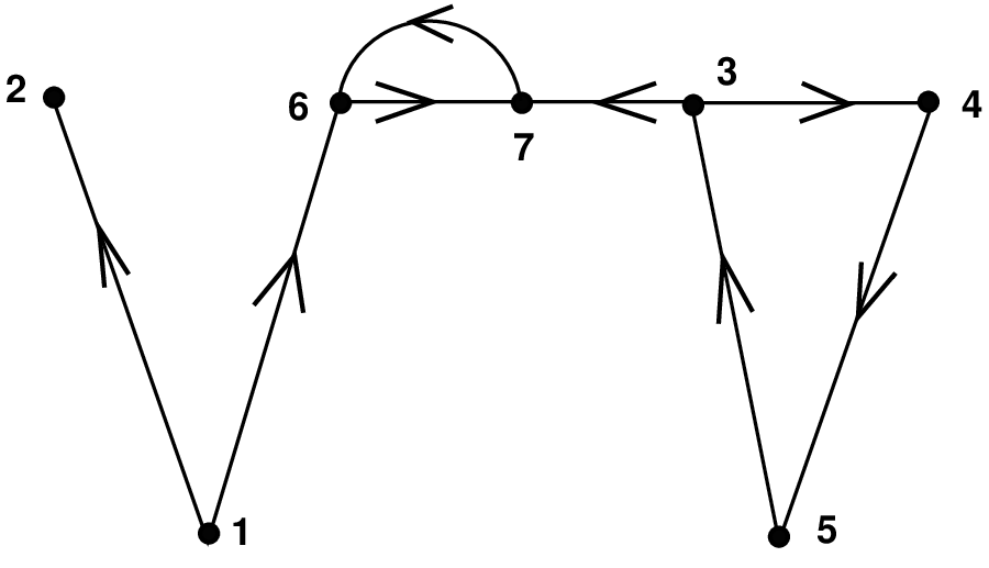
The algorithm at the beginning of Section 4 gives the stochastic matrix as
The stochastic matrix with teleporting is nearly the same: the second row entries are replaced by 1/7.
The bases of the left and right kernels of the Laplacian of Theorems 3.3 and 4.8 are, respectively,
The general solutions to both the random walk and the consensus problems are given in terms of these vectors as in Theorems 5.4 and 5.8. Note that for the former, Corollary 5.6 does not hold. In this example, the matrix is:
Thus the influence vector is
Next, we solve for the pageranks with (or ). Without teleporting we get
From this the pagerank vector follows from Theorem 6.4:
The same calculation using gives:
Notice that the teleporting decreases the rank of vertex 1 and re-distributes the remaining measure over the other vertices. It is easy to check that and (Corollary 6.10).
8 Appendix: Discrete versus Continuous Consensus
We briefly discuss the way discrete and continuous consensus relate to one another. The case of diffusion is exactly the same.
If we start with the flow defined by on a digraph then, we can easily determine its time 1 map, namely , as well as its properties. A graph is a transitive closure of the graph if for every possible (directed) path in in there is a (directed) edge in .
Proposition 8.1.
Consider a non-negative row-stochastic adjacency matrix associated
with the graph and a (rw) Laplacian
. Then
(i) is row-stochastic,
(ii) is non-negative, and
(iii) is the adjacency matrix of a transitive closure of .
Proof 8.2.
(i) From the expansion in powers of , we see that must have row sum 1. (ii) If we expand in powers of , we see that is non-negative. (iii) By (i) and (ii), we may consider as a (weighted) adjacency matrix of a graph . The entry of positive if and only if there is a path of length in . The expansion in shows that every power of S occurs with a positive coefficient. Thus the entry of is positive if and only if there is a path .
Now let us start with a time 1 map and consider the much more challenging problem of constructing (if possible) a flow that generates it. The matrix is sometimes referred as the logarithm of [20]. A stochastic matrix (or its corresponding Markov chain) for which such a flow exists is called embeddable. The problem of characterizing the embeddable stochastic matrices is known as the embedding problem for finite Markov chains and is an area of current research interest. The general problem of determining if a given stochastic matrix has such a flow has been recently shown to be NP-complete [16]. Recent characterizations for special classes of stochastic matrices can be found in [22] and [36].
There is an obvious obstruction to the construction of a continuous flow that generates a given discrete system as its time 1 map . Namely, if has an eigenvalue 0, then there is there is no flow whose time 1 map generates it. Intuitively, this is because would imply that diverges, which, as we have seen, is impossible for a laplacian . For more details we refer the reader to [20] (under logarithms of matrices).
A more interesting obstruction follows from Proposition 8.1. If the matrix does not correspond to a transitively closed graph, then the logarithm of (if it exists) cannot be rw Laplacian. Here is an example.
Perhaps surprisingly, transitive closure of the graph associated with a stochastic matrix is not sufficient to ensure that is embeddable. Examples can be found in [22]. These examples give real logarithms of which are not Laplacians. One can show that there are no other real logarithms (c.f. Theorem 2 in [17]).
Corollary 8.3.
The right kernels of an are equal. Similar for the left kernels.
Proof 8.4.
The structure of the reaches in a graph is entirely determined by the paths in that graph. Thus, the reaches and in particular their subdivision in cabals, exclusive parts, and common parts are the same for and . Thus dimension of the kernels is the same. Since kernels are linear spaces, it is sufficient to show that . So, let , then
where the last equality follows upon expanding the exponential.
Remark: As we observed above, there is one substantial difference between an . While the strongly connected components of the two are equal, the restriction of to such a component is strictly positive. That means that the matrix restricted to such a component is primitive, and no periodic behavior occurs. Hence the averaging we see in Theorem 5.4 for a discrete system is replaced by a straightforward limit for continuous systems (Theorem 5.8).
Acknowledgements.
The authors gratefully acknowledge a useful conversation with Jeff Ovall.References
- [1] BibliographyV. I. Arnold, Ordinary Differential Equations, 3rd edn (Springer, Berlin, 1992).
- [2] BibliographyR. Agaev P. Chebotarev, ‘On the spectra of non-symmetric laplacian matrices’, Lin. Alg. and its Appl. 399 (2005) 157-168
- [3] BibliographyR. Ahlswede et al., ‘Network information flow’, IEEE Transactions on Information Theory 46 (2000) no. 4, 1204-1216.
- [4] BibliographyR. Angles C. Guiterrez, ‘Survey of graph database models’, ACM Computing Surveys 40 (2008) No. 1, 1-39.
- [5] BibliographyJ. Bang-Jensen G. Gutin, Digraphs: Theory, Algorithms, and Applications, (Springer, Berlin, 2007).
- [6] BibliographyF. Bauer, ‘Normalized graph laplacians for directed graphs’, Lin. Alg. and its Appl. 436 (2012) 4193-4222.
- [7] BibliographyI. Benjamini L. Lovász, ‘Harmonic and analytic functions on graphs’, J. Geom. 76 (2003) 3-15.
- [8]
BibliographyM. Boyle, Notes on Perron-Frobenius theory of nonnegative matrices, 2005,
www.math.umd.edu/~mboyle/courses/475sp05/spec.pdf - [9] BibliographyD. Boley, G. Ranjan, Z. Zhang, ‘Commute times for a directed graph using an asymmetric laplacian’,Lin. Alg. and its Appl. 435 (2011) 224-242.
- [10] BibliographyB. Bollobás, Modern Graph Theory, (Springer, Berlin, 1998).
- [11] BibliographyA. Broder et al., ‘Graph structure of the web’,Computer Networks 33 (2000) 309-322.
- [12] BibliographyP. Carrington, J. Scott, S. Wasserman, Models and Methods in Social Network Analysis, (Cambridge University Press, Cambridge, 2005).
- [13] BibliographyJ. S. Caughman J. J. P. Veerman, ‘Kernels of directed graph laplacians’, Electronic Journal of Combinatorics 13 (2006) No 1, R39.
- [14] BibliographyF. Chung, ‘Laplacians and the Cheeger inequality for directed graphs’, Annals of Combinatorics 9 (2005) 1-19.
- [15] BibliographyF. Chung W. Zhao, ‘Pagerank and random walks of graphs‘, Fete of Combinatorics and Computer Science, (eds G. O. H. Katona, A. Schrijver and T. Szonyi.; Springer, Berlin, 2010) 43-63.
- [16] BibliographyJ. Bausch T. Cubitt, ‘The complexity of divisibility’, Lin. Alg. and its Appl. 504 (2016) 64-107.
- [17] BibliographyW. Culver, ‘On the existence and uniqueness of the real logarithm of a matrix’, Proceedings of the American Mathematical Society 17 (1966) No 5, 1146-1151.
- [18] BibliographyJ. Fax R Murray, ‘Information flow and cooperative control of vehicle formations’, IEEE Transactions on Automatic Control 49 (2004) No. 9, 1465-1476.
- [19] BibliographyJ. L. Gross, J. Zellen, P. Zhang, Handbook of Graph Theory, 2nd edn (CRC Press, Boca Raton, 2014).
- [20] BibliographyN. Higham, Functions of Matrices. Theory and Computation, (SIAM, Philadelphia, 2008).
- [21] BibliographyR. A. Horn C. R. Johnson, Matrix Analysis, 2nd Edn (Cambridge University Press, New York, 2017).
- [22] BibliographyC. Jia, ‘A solution to the reversible embedding problem for finite Markov chains’, Statistics and Probability Letters 116 (2016) 122-130.
- [23] BibliographyT. Jombert et al., ‘Reconstructing disease outbreaks from genetic data: a graph approach’,Heredity 106 (2011) 383-390.
- [24] BibliographyA. Langville C. Meyer, Google’s PageRank and Beyond, (Princeton University Press, Princeton, 2011).
- [25] BibliographyD. A. Levin Yuval Peres, Markov Chains and Mixing Times, 2nd Edn (American Mathematical Society, Providence, 2017).
- [26] BibliographyN. Masuda H. Kori, ‘Dynamics based centrality for directed networks’, Phys. Review E 82 (2010) 056107, doi:10.1103/PhysRevE.82.056107.
- [27] BibliographyN. Masuda, ‘Random walks and diffusion on networks’, Physics Reports 716-717 (2017) 1-59.
- [28] BibliographyR. M. May, ‘Qualitative stability in model ecosystems’, Ecology 54 (1973) No. 3, 638-641.
- [29] BibliographyP. McGraw M. Menzinger, ‘Laplacian spectra as a diagnostic tool for network structure and dynamics’, Physical Review E 77 (2008) 031102, doi:10.1103/PhysRevE.77.031102.
- [30] BibliographyM. Mesbahi M. Egerstedt, Graph Theoretic Methods in Multiagent Networks, (Princeton University Press, Princeton, 2010).
- [31] BibliographyI. Mirzaev J. Gunawardena, ‘Laplacian dynamics on general graphs‘, Bull. Math. Biol. (11) 75 (2013) 2118-2149.
- [32] BibliographyG. Punzo et al., ‘Using network dynamical influence to drive consensus’, Sci. Rep. 6 (2016) 26318, doi:10.1038/srep26318.
- [33] BibliographyS. Rao et al., ‘A graph-theoretical approach for the analysis and model reduction of complex-balanced chemical reaction networks’, J. Math. Chem. 51 (2013) No. 9, 2401-2422.
- [34] BibliographyS. Sternberg, Dynamical Systems, (Dover Publications, Mineola NY, 2010).
- [35] BibliographyJ. J. P. Veerman et al.,‘Flocks and formations’, J. Stat. Phys. (5-6) 121 (2005) 901-936.
- [36] BibliographyA. Van-Brunt, ‘Infinitely divisible nonnegative matrices, M-matrices, and the embedding problem for finite state stationary Markov chains’, Lin. Alg. and its Appl. 541 (2018) 163-176.
- [37] BibliographyD. Wagner, ‘The critical group of a graph’, preprint, https://arxiv.org/abs/math/0010241 Retrieved 2018.
- [38] BibliographyD. B. West, Introduction to Graph Theory, 2nd Edn (Prentice-Hall, Upper Saddle River NJ, 2001).
J. J. P. Veerman and E. Kummel
Portland State University
PO Box 751
Portland, OR 97207-0751
United States of America