跳到论文正文
W Papers独立论文阅读器 arXiv:1807.09813 论文正文 计算阅读时间 · 0%
引用这篇论文根据当前论文元数据生成,正式投稿前建议核对。


License: arXiv.org perpetual non-exclusive license
arXiv:1807.09813v4 [stat.ML] 10 Jan 2020

Binacox: automatic cut-point detection in high-dimensional Cox model with applications in genetics

Abstract

We introduce the binacox, a prognostic method to deal with the problem of detecting multiple cut-points per features in a multivariate setting where a large number of continuous features are available. The method is based on the Cox model and combines one-hot encoding with the binarsity penalty, which uses total-variation regularization together with an extra linear constraint, and enables feature selection. Original nonasymptotic oracle inequalities for prediction (in terms of Kullback-Leibler divergence) and estimation with a fast rate of convergence are established. The statistical performance of the method is examined in an extensive Monte Carlo simulation study, and then illustrated on three publicly available genetic cancer datasets. On these high-dimensional datasets, our proposed method significantly outperforms state-of-the-art survival models regarding risk prediction in terms of the C-index, with a computing time orders of magnitude faster. In addition, it provides powerful interpretability from a clinical perspective by automatically pinpointing significant cut-points in relevant variables.

Keywords. Cox model; Cut-point; Feature binarization; Nonasymptotic oracle inequality; Proximal methods; Survival analysis; Total variation

Simon Bussy
LPSM, UMR 8001, CNRS, Sorbonne University, Paris, France

email: simon.bussy@gmail.com

Mokhtar Z. Alaya
Modal’X, UPL, Univ Paris Nanterre, F92000 Nanterre, France

email: mokhtarzahdi.alaya@gmail.com

Anne-Sophie Jannot
Biomedical Informatics and Public Health Department, EGPH, APHP

and INSERM, UMRS 1138, Centre de Recherche des Cordeliers, Paris, France

email: annesophie.jannot@aphp.fr

Agathe Guilloux
LaMME, UEVE and UMR 8071, Paris Saclay University, Evry, France

email: agathe.guilloux@math.cnrs.fr

1 Introduction

Determining significant prognostic biomarkers is of increasing importance in many areas of medicine. Scores used in clinical practice often categorize continuous features into binary ones using expert-driven cut-points. For instance, the Wells score, which categorizes patients into low, moderate and high risk groups for pulmonary embolism (Wells et al., 2000), is one of the most extensively validated predictive scores. One of the categorized feature used in this score is “having a heart rate of over 100 beats per minute, or not”. When used in routine care, this type of threshold makes a score more interpretable from a clinical point of view. In this particular example, it means that experts consider that heart rate has a nonlinear effect: there is reasonable agreement that above this threshold, patients have higher risk of unfavourable outcome. Despite this choice of threshold, there is little agreement on the exact nature of the relationship between heart rate and prognosis.

With the increasing availability of high-dimensional datasets, data-driven predictive scores are becoming increasingly important, e.g., in genetic oncology studies, where similar questions occur because the effect of certain genes’ expression on survival times are often non-linear. Therefore, to develop such scores, one has to deal with a two-sided problem: first to select relevant features, and second to find relevant thresholds – also called cut-off values or cut-points – for these selected continuous features, without prior or expert knowledge.

The cut-point detection problem.

Solving this problem means applying non-linearities to feature effects that most models cannot detect. This also offers the ability to classify patients into several groups in terms of their continuous feature values relative to the cut-points. More importantly, this can also lead to a better understanding of the features’ effects on the outcome of interest; this strategy might uncover biological thresholds as well as potential criteria for new prospective studies, help diagnose diseases, and make treatment recommendations. A convenient tool for finding optimal cut-points is therefore of high interest.

Indeed, good cut-point detection is a common issue in medical studies, and numerous methods have been proposed for determining a single cut-point for a given feature. This ranges from choosing the mean or median, to methods based on distribution of values, or association with clinical outcomes, e.g., the minimal pp-value from multiple log-rank tests, see Camp et al. (2004); Moul et al. (2007); Rota et al. (2015) among many others. However, the choice of the actual cut-points is not a straightforward problem, even for a single cut-point (Lausen and Schumacher, 1992; Klein and Wu, 2003; Contal and O’Quigley, 1999). Recently, Icuma et al. (2018) proposed a Bayesian approach with accelerated failure time modeling, but still only allowing one cut-point per feature.

Indeed, while many studies have been devoted to find one optimal cut-point, there is often need in medical settings to determine not only one but multiple cut-points. For instance, prognoses are generally worst at both ends of the body mass index, i.e., for obese and underweight individuals (Oreopoulos et al., 2008). Methods exist to deal with multiple cut-point detection for one-dimensional signals (see for instance Bleakley and Vert (2011) and Harchaoui and Lévy-Leduc (2010) that use a group fused lasso or total-variation penalty, respectively), and for multivariate time series (see Cho and Fryzlewicz (2015)). Though cut-point detection is also a paramount issue in survival analysis (Faraggi and Simon, 1996), methods that have been developed in this setting only look at a single feature at a time (e.g., Motzer et al. (1999) and LeBlanc and Crowley (1993) which use survival trees, or more recently Chang et al. (2019)). To our knowledge, a multivariate survival analysis method well-suited to detect multiple cut-points per feature in a high-dimensional setting has not been previously proposed.

General framework.

Let us consider the usual survival analysis framework. Following Andersen et al. (2012), let non-negative random variables TT and CC stand for the time of the event of interest and censoring time respectively, and XX denote the pp-dimensional vector of features (e.g., patient characteristics, therapeutic strategy, omics features). The event of interest could be for instance survival time, re-hospitalization, relapse or disease progression. Conditionally on XX, TT and CC are assumed to be independent, which is classical in survival analysis (Klein and Moeschberger, 2005). We then denote ZZ the right-censored time and Δ\Delta the censoring indicator, defined as

Z=T∧CandΔ=𝟙​(T≤C)Z=T\wedge C\quad\text{and}\quad\Delta=\mathds{1}({T\leq C})

respectively, where a∧ba\wedge b denotes the minimum between two numbers aa and bb, and 𝟙​(⋅)\mathds{1}(\cdot) the indicator function taking the value 11 if the condition in (⋅)(\cdot) is satisfied and 00 otherwise.

The Cox proportional hazards model (Cox, 1972) is by far the most widely used in survival analysis. It describes the relation between the hazard function and the features by

λ⁡(t|X=x)=λ0​(t)​ex⊤​βcox,\lambda(t|X=x)=\lambda_{0}(t)e^{x^{\top}\beta^{\text{cox}}},

where λ0\lambda_{0} is a baseline hazard function describing how the event risk changes over time at baseline levels of features, and βcox∈ℝp\beta^{\text{cox}}\in{\mathbb{R}}^{p} a vector quantifying the multiplicative impact on the hazard ratio of each feature.

High-dimensional survival analysis.

High-dimensional settings are becoming increasingly frequent, in particular for genetic data applications where cut-point estimation is a common problem (see for instance Harvey et al. (1999); Shirota et al. (2001); Cheang et al. (2009)), but also in other contexts where the number of available features to consider as potential risk factors is tremendous, particularly with the development of electronic health records. A penalized version of the Cox model well-suited for such settings is proposed in Simon et al. (2011), but it cannot model nonlinearity. Theory for using lasso-type methods in the Cox model was developed in Huang et al. (2013). Other methods have been put forward to deal with this problem in similar settings, like boosting Cox models (Li and Luan, 2005) and random survival forests (Ishwaran et al., 2008). However, none of these identify cut-point values, which is of major interest for both interpretation and clinical benefit.

Main contribution.

In this paper, we propose a method called binacox that estimates multiple cut-points in a Cox model with high-dimensional features. First, the binacox one-hot encodes the continuous input features (Wu and Coggeshall, 2012) through a mapping to a new binarized space of much higher dimension, and then trains the Cox model in this space, regularized with the binarsity penalty (Alaya et al., 2017) which combines total-variation regularization with an extra sum-to-zero constraint, and enables feature selection. Cut-points of the initial continuous input features are then detected by the jumps in the regression coefficient vectors, which the binarsity penalty forces to be piecewise-constant. The main contribution of this paper is twofold. First we introduce the idea of using a total-variation penalty with an extra linear constraint on the weights of a Cox model trained on a binarization of the raw continuous features. This leads to a procedure that automatically detects relevant features and allows multiple cut-points per feature. Secondly the oracle inequality in prediction of Section 3 (see Theorem 1) is stated in terms of Kullback-Leibler divergence, as opposed to the results in Huang et al. (2013) (for the lasso penalty) expressed in Breiman divergence, the arguments are consequently different.

Organization of the paper.

A precise description of the model is given in Section 2. Section 3 highlights the good theoretical properties of the binacox by establishing fast oracle inequalities for prediction and for estimation. Section 4 presents the simulation procedure used to evaluate the performance of our method and compares it with existing ones. In Section 5, we apply our method to high-dimensional genetic datasets. Finally, we discuss the obtained results in Section 6.

Notation.

Throughout the paper, for every q>0,q>0, we denote by ‖v‖q\|v\|_{q} the usual ℓq\ell_{q}-quasi norm of a vector v∈ℝm,v\in{\mathbb{R}}^{m}, namely ‖v‖q=(∑k=1m|vk|q)1/q\|v\|_{q}=(\sum_{k=1}^{m}|v_{k}|^{q})^{1/q}, and ‖v‖∞=max1≤k≤m⁡|vk|\|v\|_{\infty}=\max_{1\leq k\leq m}|v_{k}|. We write 𝟏\mathbf{1} (resp. 𝟎\mathbf{0}) the vector having all coordinates equal to one (resp. zero). We also denote |A||A| the cardinality of a finite set AA. If II is an interval, |I||I| stands for its Lebesgue measure. Then, for any u∈ℝmu\in{\mathbb{R}}^{m} and any L⊂{1,…,m},L\subset\{1,\ldots,m\}, we denote uLu_{L} the vector of ℝm{\mathbb{R}}^{m} satisfying (uL)k=uk(u_{L})_{k}=u_{k} for k∈Lk\in L and (uL)k=0(u_{L})_{k}=0 for k∈L∁:={1,…,m}\Lk\in L^{\complement}:=\{1,\ldots,m\}\backslash L. Finally, for a matrix MM of size k×k′k\times k^{{}^{\prime}}, Mj,∙M_{j,\bullet} denotes its jjth row and M∙,lM_{\bullet,l} its llth column.

2 Model and method

2.1 Cox model with cut-points.

Consider an independent and identically distributed (i.i.d.) sample

(X1,Z1,Δ1),…,(Xn,Zn,Δn)∈[0,1]p×ℝ+×{0,1},(X_{1},Z_{1},\Delta_{1}),\dots,(X_{n},Z_{n},\Delta_{n})\in[0,1]^{p}\times{\mathbb{R}}_{+}\times\{0,1\},

where the condition Xi∈[0,1]pX_{i}\in[0,1]^{p} for all i=1,…,ni=1,\ldots,n is always true after an appropriate rescaling preprocessing step, without loss of generality. Let 𝑿=[Xi,j]1≤i≤n;1≤j≤p\boldsymbol{X}=[X_{i,j}]_{1\leq i\leq n;1\leq j\leq p} be the n×pn\times p design matrix vertically stacking the nn samples of pp raw features so that 𝑿i,∙=Xi\boldsymbol{X}_{i,\bullet}=X_{i}. In order to simplify the presentation of our results, we assume in the paper that the raw features 𝑿∙,j\boldsymbol{X}_{\bullet,j} are continuous for all j=1,…,pj=1,\ldots,p, but this is not a limitation in practice. Assume that the hazard function for patient ii is given by

λ⋆​(t|Xi)=λ0⋆​(t)​ef⋆​(Xi),\lambda^{\star}(t|X_{i})=\lambda_{0}^{\star}(t)e^{f^{\star}(X_{i})},

where λ0⋆​(t)\lambda_{0}^{\star}(t) is the baseline hazard function, and

f⋆​(Xi)=∑j=1pfj⋆​(Xi,j)=∑j=1p∑k=1Kj⋆+1βj,k⋆​𝟙​(Xi,j∈Ij,k⋆),f^{\star}(X_{i})=\sum_{j=1}^{p}f^{\star}_{j}(X_{i,j})=\sum_{j=1}^{p}\sum_{k=1}^{K_{j}^{\star}+1}\beta^{\star}_{j,k}\mathds{1}(X_{i,j}\in I^{\star}_{j,k}), (1)

with Ij,k⋆=(μj,k−1⋆,μj,k⋆]I^{\star}_{j,k}=(\mu^{\star}_{j,k-1},\mu_{j,k}^{\star}] for k=1,…,Kj⋆+1k=1,\ldots,K^{\star}_{j}+1 and where βj,k⋆≠βj,k+1⋆\beta^{\star}_{j,k}\neq\beta^{\star}_{j,k+1} for k=1,…,Kj⋆k=1,\ldots,K^{\star}_{j}. We impose that

∑i=1nfj⋆​(Xi,j)=0 for all ​j=1,…,p\sum_{i=1}^{n}f^{\star}_{j}(X_{i,j})=0\quad\text{ for all }j=1,\ldots,p

to ensure identifiability (see (Meier et al., 2009) for a similar constraint in generalized additive models), which can also be written as a sum-to-zero constraint in each β⋆\beta^{\star}’s block, that is:

∑k=1Kj⋆+1βj,k⋆​nj,k⋆=0 for all ​j=1,…,p\sum_{k=1}^{K_{j}^{\star}+1}\beta^{\star}_{j,k}n^{\star}_{j,k}=0\quad\text{ for all }j=1,\ldots,p (2)

where nj,k⋆=|{i=1,…,n:Xi,j∈Ij,k⋆}|n^{\star}_{j,k}=|\{i=1,\ldots,n:X_{i,j}\in I^{\star}_{j,k}\}|. For each feature j=1,…,pj=1,\ldots,p, the μj,k⋆\mu^{\star}_{j,k}s (k=1,…,Kj⋆k=1,\ldots,K^{\star}_{j}) are the so-called cut-points, and are such that

μj,1⋆<μj,2⋆<⋯<μj,Kj⋆⋆,\mu^{\star}_{j,1}<\mu^{\star}_{j,2}<\cdots<\mu^{\star}_{j,K^{\star}_{j}},

with the conventions μj,0⋆=0\mu^{\star}_{j,0}=0 and μj,Kj⋆+1⋆=1\mu^{\star}_{j,K^{\star}_{j}+1}=1. Denoting K⋆=∑j=1pKj⋆K^{\star}=\sum_{j=1}^{p}K^{\star}_{j}, the vector of regression coefficients β⋆∈ℝK⋆+p\beta^{\star}\in{\mathbb{R}}^{K^{\star}+p} is given by

β⋆\displaystyle\beta^{\star} =(β1,∙⋆⊤,…,βp,∙⋆⊤)⊤=(β1,1⋆,…,β1,K1⋆+1⋆,…,βp,1⋆,…,βp,Kp⋆+1⋆)⊤,\displaystyle=({\beta^{\star}_{1,\bullet}}^{\top},\ldots,{\beta^{\star}_{p,\bullet}}^{\top})^{\top}=(\beta^{\star}_{1,1},\ldots,\beta^{\star}_{1,K^{\star}_{1}+1},\ldots,\beta^{\star}_{p,1},\ldots,\beta^{\star}_{p,K_{p}^{\star}+1})^{\top},

and the cut-points vector μ⋆∈ℝK⋆\mu^{\star}\in{\mathbb{R}}^{K^{\star}} by

μ⋆\displaystyle\mu^{\star} =(μ1,∙⋆⊤,…,μp,∙⋆⊤)⊤=(μ1,1⋆,…,μ1,K1⋆⋆,…,μp,1⋆,…,μp,Kp⋆⋆)⊤.\displaystyle=({\mu^{\star}_{1,\bullet}}^{\top},\ldots,{\mu^{\star}_{p,\bullet}}^{\top})^{\top}=(\mu^{\star}_{1,1},\ldots,\mu^{\star}_{1,K^{\star}_{1}},\ldots,\mu^{\star}_{p,1},\ldots,\mu^{\star}_{p,K^{\star}_{p}})^{\top}.

Our goal is to simultaneously estimate μ⋆\mu^{\star} and β⋆\beta^{\star}, which also requires estimation of the unknown Kj⋆K^{\star}_{j} for all j=1,…,pj=1,\ldots,p. Towards this end, the first step of our proposed method is to map the feature space to a much higher space of binarized features.

2.2 Binarization.

Let 𝑿B{\boldsymbol{X}}^{B} be the sparse binarized matrix with an extended number p+dp+d of columns, typically with d≫pd\gg p, where continuous input features have been one-hot encoded (Wu and Coggeshall, 2012; Liu et al., 2002). The jjth column 𝑿∙,j\boldsymbol{X}_{\bullet,j} is then replaced by dj+1≥2d_{j}+1\geq 2 columns 𝑿∙,j,1B,…,𝑿∙,j,dj+1B\boldsymbol{X}^{B}_{\bullet,j,1},\ldots,\boldsymbol{X}^{B}_{\bullet,j,d_{j}+1} containing only zeros and ones, where the iith row XiB∈ℝp+dX_{i}^{B}\in{\mathbb{R}}^{p+d} with d=∑j=1pdjd=\sum_{j=1}^{p}d_{j} is written

XiB=(Xi,1,1B,…,Xi,1,d1+1B,…,Xi,p,1B,…,Xi,p,dp+1B)⊤.X_{i}^{B}=(X^{B}_{i,1,1},\ldots,X^{B}_{i,1,d_{1}+1},\ldots,X^{B}_{i,p,1},\ldots,X^{B}_{i,p,d_{p}+1})^{\top}.

We consider a partition of intervals Ij,1,…,Ij,dj+1I_{j,1},\ldots,I_{j,d_{j}+1} such that

⋃k=1dj+1Ij,k=[0,1]\bigcup_{k=1}^{d_{j}+1}I_{j,k}=[0,1]

and Ij,k∪Ij,k′=∅I_{j,k}\cup I_{j,k^{\prime}}=\varnothing for all k≠k′k\neq k^{\prime} with k,k′=1,…,dj+1k,k^{\prime}=1,\ldots,d_{j}+1. Now for i=1,…,ni=1,\ldots,n and l=1,…,dj+1l=1,\ldots,d_{j}+1, we define

Xi,j,lB={1 if ​Xi,j∈Ij,l,0 otherwise.X_{i,j,l}^{B}=\begin{cases}1&\text{ if }X_{i,j}\in I_{j,l},\\ 0&\text{ otherwise}.\end{cases}

We then denote Ij,l=(μj,l−1,μj,l]I_{j,l}=(\mu_{j,l-1},\mu_{j,l}] for l=1,…,dj+1l=1,\ldots,d_{j}+1, with the convention μj,0=0\mu_{j,0}=0 and μj,dj+1=1\mu_{j,d_{j}+1}=1. A natural choice for the μj,l\mu_{j,l} is given by the quantiles, namely μj,l=qj​(l/(dj+1))\mu_{j,l}=q_{j}\big(l/(d_{j}+1)\big), where qj​(α)q_{j}(\alpha) denotes a quantile of order α∈[0,1]\alpha\in[0,1] for 𝑿∙,j\boldsymbol{X}_{\bullet,j}. If training data also contains unordered qualitative features, one-hot encoding with ℓ1\ell_{1}-penalization can be used, for instance.

To each binarized feature 𝑿∙,j,lB\boldsymbol{X}^{B}_{\bullet,j,l} corresponds a parameter βj,l\beta_{j,l}, and the vectors associated with the binarization of the jjth feature are naturally denoted βj,∙=(βj,1,…,βj,dj+1)⊤\beta_{j,\bullet}=(\beta_{j,1},\ldots,\beta_{j,d_{j}+1})^{\top} and μj,∙=(μj,1,…,μj,dj)⊤\mu_{j,\bullet}=(\mu_{j,1},\ldots,\mu_{j,d_{j}})^{\top}. Hence, we define a candidate for the estimation of f⋆f^{\star} defined in (1) as

fβ​(Xi)=β⊤​XiB=∑j=1pfβj,∙​(Xi,j)=∑j=1p∑l=1dj+1βj,l​𝟙​(Xi,j∈Ij,l).f_{\beta}(X_{i})=\beta^{\top}{X_{i}^{B}}=\sum_{j=1}^{p}f_{\beta_{j,\bullet}}(X_{i,j})=\sum_{j=1}^{p}\sum_{l=1}^{d_{j}+1}\beta_{j,l}\mathds{1}(X_{i,j}\in I_{j,l}). (3)

The full parameter vectors of size p+dp+d and dd respectively are finally obtained by concatenation of the vectors βj,∙\beta_{j,\bullet} and μj,∙\mu_{j,\bullet}, i.e.,

β\displaystyle\beta =(β1,∙⊤,…,βp,∙⊤)⊤=(β1,1,…,β1,d1+1,…,βp,1,…,βp,dp+1)⊤,\displaystyle=(\beta_{1,\bullet}^{\top},\ldots,\beta_{p,\bullet}^{\top})^{\top}=(\beta_{1,1},\ldots,\beta_{1,d_{1}+1},\ldots,\beta_{p,1},\ldots,\beta_{p,d_{p}+1})^{\top},

and

μ\displaystyle\mu =(μ1,∙⊤,…,μp,∙⊤)⊤=(μ1,1,…,μ1,d1,…,μp,1,…,μp,dp)⊤.\displaystyle=(\mu_{1,\bullet}^{\top},\ldots,\mu_{p,\bullet}^{\top})^{\top}=(\mu_{1,1},\ldots,\mu_{1,d_{1}},\ldots,\mu_{p,1},\ldots,\mu_{p,d_{p}})^{\top}.

2.3 Estimation procedure.

In the following, for a fixed vector μ\mu of quantization, we define the binarized partial negative log-likelihood (rescaled by 1/n1/n) as follows:

ℓn(fβ)=−1n∑i=1nΔi{fβ(Xi)−log∑i′:Zi′≥Ziefβ​(Xi′)}.\displaystyle\ell_{n}(f_{\beta})=-\frac{1}{n}\sum_{i=1}^{n}\Delta_{i}\Big\{f_{\beta}(X_{i})-\log\sum_{\begin{subarray}{c}i^{\prime}:Z_{i^{\prime}}\geq Z_{i}\end{subarray}}e^{f_{\beta}(X_{i^{\prime}})}\Big\}. (4)

Our approach consists in minimizing the function ℓn\ell_{n} plus the binarsity penalization term introduced in Alaya et al. (2017). The resulting optimization problem is written

β^∈argminβ∈ℬp+d​(R)⁡{ℓn​(fβ)+bina⁡(β)},\hat{\beta}\in\argmin_{\beta\in\mathscr{B}_{p+d}(R)}\big\{\ell_{n}(f_{\beta})+\bina(\beta)\big\}, (5)

where ℬp+d​(R)={β∈ℝp+d:∑j=1p‖βj,∙‖∞≤R}\mathscr{B}_{p+d}(R)=\{\beta\in{\mathbb{R}}^{p+d}:\sum_{j=1}^{p}\|\beta_{j,\bullet}\|_{\infty}\leq R\} and

bina⁡(β)=∑j=1p(∑l=2dj+1ωj,l​|βj,l−βj,l−1|+δj​(βj,∙)),\bina(\beta)=\sum_{j=1}^{p}\Big(\sum_{l=2}^{d_{j}+1}\omega_{j,l}|\beta_{j,l}-\beta_{j,{l-1}}|+\delta_{j}(\beta_{j,\bullet})\Big), (6)

with

δj​(u)={0 if nj,∙⊤​u=0,∞ otherwise,\delta_{j}(u)=\begin{cases}0\quad&\text{ if }\quad n^{\top}_{j,\bullet}u=0,\\ \infty&\text{ otherwise,}\end{cases}

and where nj,∙=(nj,1,…,nj,dj+1)⊤∈ℕdj+1n_{j,\bullet}=(n_{j,1},\ldots,n_{j,d_{j}+1})^{\top}\in\mathbb{N}^{d_{j}+1} with nj,l=|{i=1,…,n:Xi,j∈Ij,l}|n_{j,l}=|\{i=1,\ldots,n:X_{i,j}\in I_{j,l}\}| for all j=1,…,pj=1,\ldots,p and l=1,…,dj+1.l=1,\ldots,d_{j}+1. The constraint over ℬp+d​(R)\mathscr{B}_{p+d}(R) is standard in the literature for obtaining proofs of oracle inequalities for sparse generalized linear models (Van de Geer, 2008), and is discussed in detail below. The weights ωj,l\omega_{j,l} are of order

ωj,l=𝒪⁡(log⁡(p+d)n),\omega_{j,l}=\mathcal{O}\bigg(\sqrt{\frac{\log(p+d)}{n}}\bigg),

see Appendix B.1 for their explicit form.

It turns out that the binarsity penalty is well-suited to our problem. First, it tackles the problem that 𝑿B{\boldsymbol{X}}^{B} is not full rank by construction, since ∑l=1dj+1Xi,j,lB=1\sum_{l=1}^{d_{j}+1}X_{i,j,l}^{B}=1 for all j=1,…,pj=1,\ldots,p, which means that the columns in each block sum to 𝟏\mathbf{1}. This problem is solved since the penalty imposes the linear constraint ∑l=1dj+1nj,l​βj,l=0\sum_{l=1}^{d_{j}+1}n_{j,l}\beta_{j,l}=0 in each block with the δj​(⋅)\delta_{j}(\cdot) term. Note that if the Ij,lI_{j,l} are taken as the interquantiles intervals, we have that nj,ln_{j,l} are all equal for l=1,…,dj+1l=1,\ldots,d_{j}+1, and we get the standard sum-to-zero constraint ∑l=1dj+1βj,l=0\sum_{l=1}^{d_{j}+1}\beta_{j,l}=0. Then, the other term in the penalty consists of a within-block weighted total variation penalty:

‖βj,∙‖TV,ωj,∙=∑l=2dj+1ωj,l​|βj,l−βj,l−1|,\|\beta_{j,\bullet}\|_{\TV,\omega_{j,\bullet}}=\sum_{l=2}^{d_{j}+1}\omega_{j,l}|\beta_{j,l}-\beta_{j,l-1}|, (7)

that takes advantage of the fact that within each block, binarized features are ordered. The effect is then to keep the number of different values taken by βj,∙\beta_{j,\bullet} to a minimum, which makes significant cut-points appear, as detailed hereafter.

For all β∈ℝp+d,\beta\in{\mathbb{R}}^{p+d}, let 𝒜⁡(β)=[𝒜1​(β),…,𝒜p​(β)]\mathcal{A}(\beta)=\big[\mathcal{A}_{1}(\beta),\ldots,\mathcal{A}_{p}(\beta)\big] be the concatenation of the support sets relative to the total-variation penalization, namely

𝒜j(β)={l:βj,l≠βj,l−1, for l=2,…,dj+1}\mathcal{A}_{j}(\beta)=\big\{l:\beta_{j,l}\neq\beta_{j,l-1},\textrm{ for }l=2,\ldots,d_{j}+1\big\}

for all j=1,…,pj=1,\ldots,p. Similarly, we denote 𝒜∁​(β)=[𝒜1∁​(β),…,𝒜p∁​(β)]\mathcal{A}^{\complement}(\beta)=\big[\mathcal{A}_{1}^{\complement}(\beta),\ldots,\mathcal{A}_{p}^{\complement}(\beta)\big] the complementary set of 𝒜⁡(β).\mathcal{A}(\beta). We then write

𝒜j​(β^)={l^j,1,…,l^j,sj},{\mathcal{A}}_{j}(\hat{\beta})=\{\hat{l}_{j,1},\ldots,\hat{l}_{j,s_{j}}\}, (8)

where l^j,1<⋯<l^j,sj\hat{l}_{j,1}<\cdots<\hat{l}_{j,s_{j}} and sj=|𝒜j​(β^)|s_{j}=|{\mathcal{A}}_{j}(\hat{\beta})|. Finally, we obtain the following μj,∙⋆\mu^{\star}_{j,\bullet}’s estimator

μ^j,∙=(μj,l^j,1,…,μj,l^j,sj)⊤\widehat{\mu}_{j,\bullet}=(\mu_{j,\hat{l}_{j,1}},\ldots,\mu_{j,\hat{l}_{j,s_{j}}})^{\top} (9)

for all j=1,…,pj=1,\ldots,p. By construction, Kj⋆K^{\star}_{j} is estimated by K^j=sj\widehat{K}_{j}=s_{j}. Some details on the algorithm used to solve the regularization problem (5) are given in Appendix A.1.

3 Theoretical guarantees

3.1 Oracle inequality for prediction

This section is devoted to a first theoretical result. In order to evaluate the prediction error, we first define the (empirical) Kullback-Leibler divergence (Senoussi, 1990) K​LnKL_{n} between the true function f⋆f^{\star} and any candidate ff as

K​Ln​(f⋆,f)=1n​∑i=1n∫0τlog⁡{ef⋆​(Xi)​∑i=1nYi​(t)​ef⁡(Xi)ef⁡(Xi)​∑i=1nYi​(t)​ef⋆​(Xi)}​Yi​(t)​λ0⋆​(t)​ef⋆​(Xi)​𝑑t,KL_{n}(f^{\star},f)=\frac{1}{n}\sum_{i=1}^{n}\int_{0}^{\tau}\log\bigg\{\frac{e^{f^{\star}(X_{i})}\sum_{i=1}^{n}Y_{i}(t)e^{f(X_{i})}}{e^{f(X_{i})}\sum_{i=1}^{n}Y_{i}(t)e^{f^{\star}(X_{i})}}\bigg\}Y_{i}(t)\lambda_{0}^{\star}(t)e^{f^{\star}(X_{i})}\mathrm{d}t, (10)

where we denote Yi​(t)=𝟙​(Zi≥t)Y_{i}(t)=\mathds{1}(Z_{i}\geq t) the at-risk process, and τ>0\tau>0 is to be defined later.

We seek to establish an oracle inequality expressed in terms of a compatibility factor (Van de Geer and Bühlmann, 2009) satisfied by the following non-negative symmetric matrix:

Σn​(f⋆,τ)=1n​∑i=1n∫0τ(XiB−X¯n​(s))​(XiB−X¯n​(s))⊤​yi​(s)​ef⋆​(Xi)​λ0⋆​(s)​𝑑s,\Sigma_{n}(f^{\star},\tau)=\frac{1}{n}\sum_{i=1}^{n}\int_{0}^{\tau}\big(X_{i}^{B}-\bar{X}_{n}(s)\big)\big(X_{i}^{B}-\bar{X}_{n}(s)\big)^{\top}y_{i}(s)e^{f^{\star}(X_{i})}\lambda_{0}^{\star}(s)\mathrm{d}s, (11)

where

X¯n​(s)=∑i=1nXiB​yi​(s)​ef⋆​(Xi)∑i=1nyi​(s)​ef⋆​(Xi)\bar{X}_{n}(s)=\frac{\sum_{i=1}^{n}X_{i}^{B}y_{i}(s)e^{f^{\star}(X_{i})}}{\sum_{i=1}^{n}y_{i}(s)e^{f^{\star}(X_{i})}}

and

yi​(s)=𝔼⁡[Yi​(s)|Xi]​ for all ​0≤s≤t​ and all ​i=1,…,n.y_{i}(s)=\mathds{E}[Y_{i}(s)|X_{i}]\text{ for all }0\leq s\leq t\text{ and all }i=1,\ldots,n.

For any concatenation of index subsets L=[L1,…,Lp]L=[L_{1},\ldots,L_{p}], we define the compatibility factor

κτ​(L)=infβ∈𝒞TV,ω​(L)\{𝟘}β⊤​Σn​(f⋆,τ)​β‖βL‖2,\kappa_{\tau}(L)=\inf\limits_{\beta\in\mathscr{C}_{\TV,\omega}(L)\backslash\{\mathbb{0}\}}\frac{\sqrt{\beta^{\top}\Sigma_{n}(f^{\star},\tau)\beta}}{\|\beta_{L}\|_{2}}, (12)

where

𝒞TV,ω​(L)={β∈ℬp+d​(R):∑j=1p‖(βj,∙)Lj∁‖TV,ωj,∙≤3​∑j=1p‖(βj,∙)Lj‖TV,ωj,∙}\mathscr{C}_{\TV,\omega}(L)\stackrel{{\scriptstyle}}{{=}}\Big\{\beta\in\mathscr{B}_{p+d}(R):\sum_{j=1}^{p}\|(\beta_{j,\bullet})_{L^{\complement}_{j}}\|_{\TV,\omega_{j,\bullet}}\leq 3\sum_{j=1}^{p}\|(\beta_{j,\bullet})_{L_{j}}\|_{\TV,\omega_{j,\bullet}}\Big\}

is a cone composed of all vectors with similar support LL.

Assumption 1

τ\tau is hereafter assumed to satisfy

max⁡∫0τ1≤i≤n⁡λ⋆​(t|Xi)​𝑑t​<∞ and min1≤i≤n⁡ℙ⁡(Ci>τ|Xi)>​0.\displaystyle\max_{1\leq i\leq n}\int_{0}^{\tau}\lambda^{\star}(t|X_{i})\mathrm{d}t<\infty\quad\text{ and }\quad\min_{1\leq i\leq n}\mathbb{P}(C_{i}>\tau|X_{i})>0.

Such assumptions on τ\tau are common in survival analysis, see e.g., Andersen et al. (2012) and Lemler (2016). We refer the reader to Gill (1983) for a discussion on the role of τ.\tau. In addition, we define cZ:=min1≤i≤n⁡yi​(τ)c_{Z}:=\min_{1\leq i\leq n}y_{i}(\tau) and remark that

cZ≥exp⁡(−max⁡∫0τ1≤i≤n⁡λ⋆​(t|Xi)​𝑑t)​min1≤i≤n⁡ℙ⁡(Ci>τ|Xi)>0.c_{Z}\geq\exp\big(-\max_{1\leq i\leq n}\int_{0}^{\tau}\lambda^{\star}(t|X_{i})\mathrm{d}t\big)\min_{1\leq i\leq n}\mathbb{P}(C_{i}>\tau|X_{i})>0.

For the sake of simplicity, we introduce the additional notation:

f∞⋆\displaystyle f^{\star}_{\infty} =max1≤i≤n|f⋆(Xi)|,s(0)(τ)=n−1∑i=1nyi(τ)ef⋆​(Xi), and Λ0⋆(τ)=∫0τλ0⋆(s)ds.\displaystyle=\max_{1\leq i\leq n}|f^{\star}(X_{i})|,\quad s^{(0)}(\tau)=n^{-1}\sum_{i=1}^{n}y_{i}(\tau)e^{f^{\star}(X_{i})},\quad\text{ and }\quad\Lambda^{\star}_{0}(\tau)=\int_{0}^{\tau}\lambda_{0}^{\star}(s)\mathrm{d}s.
Assumption 2

Let ε∈(0,1)\varepsilon\in(0,1) and define tn,p,d,εt_{n,p,d,\varepsilon} as the solution of

2.221(p+d)2exp{−ntn,p,d,ε2/(2+2tn,p,d,ε/3)}=ε.2.221(p+d)^{2}\exp\{-nt^{2}_{n,p,d,\varepsilon}/(2+2t_{n,p,d,\varepsilon}/3)\}=\varepsilon.

For any concatenation set L=[L1,…,Lp]L=[L_{1},\ldots,L_{p}] such that ∑j=1p|Lj|≤K⋆\sum_{j=1}^{p}|L_{j}|\leq K^{\star}, assume that

κτ2​(L)>Ξτ​(L),\kappa^{2}_{\tau}(L)>\Xi_{\tau}(L),

where

Ξτ(L)=4|L|(8​maxj⁡(dj+1)​maxj,l​ωj​lminj,l⁡ωj,l)2{\displaystyle\Xi_{\tau}(L)=4|L|\Big(\frac{8\max_{j}(d_{j}+1)\max_{j,l}\omega_{jl}}{\min_{j,l}\omega_{j,l}}\Big)^{2}\Big\{ (1+e2​f∞⋆​Λ0⋆​(τ))​(2/n)​log⁡(2​(p+d)2/ε)\displaystyle\big(1+e^{2f^{\star}_{\infty}}\Lambda^{\star}_{0}(\tau)\big)\sqrt{(2/n)\log\big(2(p+d)^{2}/\varepsilon\big)}
+(2e2​f∞⋆Λ0⋆(τ)/s(0)(τ))tn,p,d,ε2}.\displaystyle+\big(2e^{2f^{\star}_{\infty}}\Lambda^{\star}_{0}(\tau)/s^{(0)}(\tau)\big)t^{2}_{n,p,d,\varepsilon}\Big\}.

Note that κτ2​(L)\kappa^{2}_{\tau}(L) is the smallest eigenvalue of a population integrated covariance matrix defined in (11), so it is reasonable to treat it as a constant. Moreover, tn,p,d,ε2t^{2}_{n,p,d,\varepsilon} is of order

1n​log⁡(p+d)2ε,\dfrac{1}{n}\log\dfrac{(p+d)^{2}}{\varepsilon},

so if |L|​log⁡(p+d)/n|L|\log(p+d)/n is sufficiently small, Assumption 2 is verified. With these preparations made, let us now state the oracle inequality for prediction satisfied by our estimator of f⋆f^{\star} which is, by construction, given by f^=fβ^\hat{f}=f_{\hat{\beta}} (see (3)).

Theorem 1

The inequality

K​Ln​(f⋆,fβ^)≤\displaystyle KL_{n}(f^{\star},f_{\hat{\beta}})\leq infβ{3​K​Ln​(f⋆,fβ)+1024​(f∞⋆+R+2)κτ2​(𝒜⁡(β))−Ξτ​(𝒜⁡(β))​|𝒜⁡(β)|​max1≤j≤p​‖(ωj,∙)𝒜j​(β)‖∞2}\displaystyle\inf_{\beta}\bigg\{3KL_{n}(f^{\star},f_{\beta})+\frac{1024(f^{\star}_{\infty}+R+2)}{{{\kappa}^{2}_{\tau}\big(\mathcal{A}({\beta})\big)-\Xi_{\tau}\big(\mathcal{A}({\beta})\big)}}|\mathcal{A}(\beta)|\max_{1\leq j\leq p}\|(\omega_{j,\bullet})_{\mathcal{A}_{j}(\beta)}\|^{2}_{\infty}\bigg\} (13)

holds with a probability greater than 1−28.55e−c−e−ns(0)(τ)2/8e2​f∞⋆−3ε1-28.55e^{-c}-e^{-ns^{(0)}(\tau)^{2}/8e^{2f^{\star}_{\infty}}}-3\varepsilon for some c>0c>0, where the infimum is over the set of vectors β∈ℬp+d​(R)\beta\in\mathscr{B}_{p+d}(R) such that nj,∙⊤​βj,∙=0n_{j,\bullet}^{\top}\beta_{j,\bullet}=0 for all j=1,…,pj=1,\ldots,p, and such that |𝒜⁡(β)|≤K⋆|\mathcal{A}(\beta)|\leq K^{\star}.

The proof of Theorem 1 is postponed to Appendix B.3. The second term in the right-hand side of (13) can be viewed as a “variance” (or “complexity”) term, and its dominant term satisfies

|𝒜⁡(β)|​maxj​‖(ωj,∙)𝒜j​(β)‖∞2κτ2​(𝒜⁡(β))−Ξτ​(𝒜⁡(β))≲|𝒜⁡(β)|κτ2​(𝒜⁡(β))−Ξτ​(𝒜⁡(β))​log⁡(p+d)n,\frac{|\mathcal{A}({\beta})|\max_{j}\|(\omega_{j,\bullet})_{\mathcal{A}_{j}(\beta)}\|^{2}_{\infty}}{\kappa^{2}_{\tau}\big(\mathcal{A}(\beta)\big)-\Xi_{\tau}\big(\mathcal{A}(\beta)\big)}\lesssim\frac{|\mathcal{A}({\beta})|}{\kappa^{2}_{\tau}\big(\mathcal{A}(\beta)\big)-\Xi_{\tau}\big(\mathcal{A}(\beta)\big)}\frac{\log(p+d)}{n},

where the symbol ≲\lesssim means that the inequality holds up to a multiplicative constant. Then, one obtains the expected fast convergence rate 𝒪⁡(log⁡(p+d)/n)\mathcal{O}\big(\log(p+d)/n\big) for the estimator f^\hat{f}. Note that, in the proof of Theorem 1, the fact that the true f⋆f^{\star} lies in the true Cox model with cut-points is not necessary. Hence Theorem 1 can be applied to any f⋆f^{\star}.

The value |𝒜⁡(β)||\mathcal{A}({\beta})| characterizes the sparsity of the vector β\beta, since it counts the number of non-equal consecutive values of β\beta. If β\beta is block-sparse, namely whenever |𝒜⁡(β)|≪p|\mathscr{A}(\beta)|\ll p where 𝒜(β)={j=1,…,p:βj,∙≠0}\mathscr{A}(\beta)=\{j=1,\ldots,p:\beta_{j,\bullet}\neq\textbf{0}\} (meaning that few raw features are useful for prediction), then |𝒜⁡(β)|≤|𝒜⁡(β)​|maxj∈𝒜⁡(β)|​𝒜j​(β)||\mathcal{A}(\beta)|\leq|\mathscr{A}(\beta)|\max_{j\in\mathscr{A}(\beta)}|\mathcal{A}_{j}(\beta)|, which means that |𝒜⁡(β)||\mathcal{A}(\beta)| is controlled by the block sparsity |𝒜⁡(β)||\mathscr{A}(\beta)|. Also, the oracle inequality still holds for vectors such that nj,∙⊤​βj,∙=0n_{j,\bullet}^{\top}\beta_{j,\bullet}=0, which is natural since the binarsity penalization imposes these extra linear constraints.

The assumption β∈ℬp+d​(R)\beta\in\mathscr{B}_{p+d}(R) is a technical one, allowing a connection, via the notion of self-concordance (Bach, 2010), between the empirical squared ℓ2\ell_{2}-norm and the empirical Kullback-Leibler (see Lemma 3). Also, note that

max1≤i≤n⁡|β⊤​XiB|≤∑j=1p‖βj,∙‖∞≤|𝒜⁡(β)|×‖β‖∞,\max_{1\leq i\leq n}|\beta^{\top}X_{i}^{B}|\leq\sum_{j=1}^{p}\|\beta_{j,\bullet}\|_{\infty}\leq|\mathscr{A}(\beta)|\times\|\beta\|_{\infty}, (14)

where ‖β‖∞=max1≤j≤p⁡‖βj,∙‖∞\|\beta\|_{\infty}=\max_{1\leq j\leq p}\|\beta_{j,\bullet}\|_{\infty}. The first inequality in (14) comes from the fact that the entries of 𝑿B{\boldsymbol{X}}^{B} are in {0,1}\{0,1\}, and entails that max1≤i≤n⁡|β⊤​XiB|≤R\max_{1\leq i\leq n}|\beta^{\top}X_{i}^{B}|\leq R whenever β∈ℬp+d​(R)\beta\in\mathscr{B}_{p+d}(R).

The second inequality in (14) shows that RR can be upper bounded by |𝒜⁡(β)|×‖β‖∞|\mathscr{A}(\beta)|\times\|\beta\|_{\infty}, and therefore the constraint β∈ℬp+d​(R)\beta\in\mathscr{B}_{p+d}(R) becomes merely a box constraint on β\beta, which depends on the dimensionality of the features through |𝒜⁡(β)||\mathscr{A}(\beta)| only. The fact that the procedure depends on RR, and that the oracle inequality stated in Theorem 1 depends linearly on RR, is commonly found in the literature on sparse generalized linear models, see Van de Geer (2008); Bach (2010); Ivanoff et al. (2016). However, the constraint ℬp+d​(R)\mathscr{B}_{p+d}(R) is a technicality which is not used in the numerical experiments in Sections 4 and 5.

Notice in addition that our proof is different from that of Huang et al. (2013) and could be applied in their setting (lasso in the Cox model with time-dependent covariates). Alternative oracle inequalities, in terms of the Kullback-Leibler divergence instead of the symmetric Bregman divergence, could hence be proven.

3.2 Oracle inequality for estimation

Approximation of f⋆f^{\star}.

Since β⋆∈ℝp+K⋆\beta^{\star}\in{\mathbb{R}}^{p+K^{\star}} and β^∈ℝp+d\hat{\beta}\in{\mathbb{R}}^{p+d}, we define in this section an approximation of f⋆f^{\star} denoted fb⋆f_{b^{\star}} with b⋆∈ℝp+db^{\star}\in{\mathbb{R}}^{p+d}. We choose djd_{j} such that

min1≤k≤Kj⋆+1⁡|Ij,k⋆|≥max1≤l≤dj+1|Ij,l|for all ​j=1,…,p.\min_{1\leq k\leq K^{\star}_{j}+1}|I^{\star}_{j,k}|\geq\max_{1\leq l\leq d_{j}+1}|I_{j,l}|\;\text{for all }j=1,\ldots,p.

This choice ensures that for all features j=1,…,pj=1,\ldots,p, there exists a unique interval Ij,lI_{j,l} containing cut-point μj,k⋆\mu^{\star}_{j,k}, which we denote

Ij,lj,k⋆=(μj,lj,k⋆−1,μj,lj,k⋆]I_{j,l^{\star}_{j,k}}=(\mu_{j,l^{\star}_{j,k}-1},\mu_{j,l^{\star}_{j,k}}] (15)

for all k=1,…,Kj⋆k=1,\ldots,K_{j}^{\star}. Note that in practice, this requirement is met by increasing djd_{j}. For each single jjth block, let us recall that as defined in (1), we associate with βj,∙⋆\beta^{\star}_{j,\bullet} the μj,∙⋆\mu_{j,\bullet}^{\star}-piecewise constant function

fj⋆:x↦∑k=1Kj⋆+1βj,k⋆​𝟙​(x∈Ij,k⋆)f^{\star}_{j}:x\mapsto\sum_{k=1}^{K^{\star}_{j}+1}\beta^{\star}_{j,k}\mathds{1}(x\in I^{\star}_{j,k})

defined for all x∈[0,1]x\in[0,1]. Now, let us define the μj,∙\mu_{j,\bullet}-piecewise constant function

f~j:x↦∑k=1Kj⋆+1βj,k⋆​∑l=lj,k−1⋆+1lj,k⋆𝟙​(x∈Ij,l),\tilde{f}_{j}:x\mapsto\sum_{k=1}^{K^{\star}_{j}+1}\beta^{\star}_{j,k}\sum_{l=l^{\star}_{j,k-1}+1}^{l^{\star}_{j,k}}\mathds{1}(x\in I_{j,l}), (16)

for x∈[0,1]x\in[0,1], where lj,k⋆l^{\star}_{j,k} is defined in (15), and with the conventions lj,0⋆=0l^{\star}_{j,0}=0 and lj,Kj⋆+1⋆=dj+1l^{\star}_{j,K^{\star}_{j}+1}=d_{j}+1 for all j=1,…,pj=1,\ldots,p. With this definition, f~j\tilde{f}_{j} has the same number of jumps and amplitudes thereof as fj⋆f^{\star}_{j}. The only difference between these two functions is the location of the jumps: fj⋆f^{\star}_{j} jumps once for each cut-point μj,k⋆\mu^{\star}_{j,k} for all k=1,…,Kj⋆+1k=1,\ldots,K^{\star}_{j}+1, while f~j\tilde{f}_{j} jumps once for each μj,l\mu_{j,l} closest (on the right hand side) to μj,k⋆\mu^{\star}_{j,k} for all k=1,…,Kj⋆+1k=1,\ldots,K^{\star}_{j}+1. This choice of approximation is discussed at the beginning of Appendix C.

In the jjth block, the vector associated with f~j\tilde{f}_{j} now lives in ℝdj+1{\mathbb{R}}^{d_{j}+1} as expected, but the extra linear constraint required to apply Theorem 1 is not fulfilled. We then define

fbj,∙⋆:x↦f~j​(x)−1n​∑i=1nf~j​(Xi,j)f_{b^{\star}_{j,\bullet}}:x\mapsto\tilde{f}_{j}(x)-\frac{1}{n}\sum_{i=1}^{n}\tilde{f}_{j}(X_{i,j}) (17)

for x∈[0,1]x\in[0,1], which gives rise to nj,∙⊤​bj,∙⋆=0n_{j,\bullet}^{\top}b^{\star}_{j,\bullet}=0 for all j=1,…,pj=1,\ldots,p, where bj,∙⋆∈ℝdj+1b^{\star}_{j,\bullet}\in{\mathbb{R}}^{d_{j}+1} is the vector associated with fbj,∙⋆f_{b^{\star}_{j,\bullet}}.

Denoting b⋆=((b1,∙⋆)⊤,…,(bp,∙⋆)⊤)⊤b^{\star}=\big((b^{\star}_{1,\bullet})^{\top},\ldots,(b^{\star}_{p,\bullet})^{\top}\big)^{\top}, our approach to prove the oracle inequality for estimation relies on the application of Theorem 1 to the approximate candidate b⋆∈ℝp+db^{\star}\in{\mathbb{R}}^{p+d} of β⋆\beta^{\star}. Figure 1 gives a clearer view of the different quantities involved so far in the estimation procedure on a toy example. See also the upper part of Figure 4 in Section 4.4. Note that, in addition, if β⋆\beta^{\star} is block-sparse, then it is also the case for b⋆b^{\star}, and the following holds:

|𝒜⁡(b⋆)|≤|𝒜⁡(β⋆)|.|\mathscr{A}(b^{\star})|\leq|\mathscr{A}(\beta^{\star})|.
Fig. 1: Illustration of the different vectors for the jjth block, with dj=17d_{j}=17. In this scenario, the algorithm detects an extra cut-point and K^j=5=sj\widehat{K}_{j}=5=s_{j}, while Kj⋆=4K^{\star}_{j}=4.

Let us introduce some further notation. We define

πn=|{i=1,…,n:Ni(τ)=1}|n,\pi_{n}=\frac{|\{i=1,\ldots,n:N_{i}(\tau)=1\}|}{n}, (18)

and let in addition

R⋆=∑j∈𝒜⁡(β⋆)‖bj,∙⋆‖∞,R^{\star}=\sum_{j\in\mathscr{A}(\beta^{\star})}\|b^{\star}_{j,\bullet}\|_{\infty},
𝐈=2​(|𝒜⁡(β⋆)|+K⋆)​(1+3​ψ⁡(f∞⋆+R⋆+2)f∞⋆+R⋆+2)​πn​maxj∈𝒜⁡(β⋆)​‖βj,∙‖∞2​maxj∈𝒜⁡(β⋆)​‖nj,∙/n‖∞2​(1+4​e2​f∞⋆cZ),{\bf{I}}=2\big(|\mathscr{A}(\beta^{\star})|+K^{\star}\big)\Big(1+3\frac{\psi(f_{\infty}^{\star}+R^{\star}+2)}{f_{\infty}^{\star}+R^{\star}+2}\Big)\pi_{n}\max_{j\in\mathscr{A}(\beta^{\star})}\|\beta_{j,\bullet}\|^{2}_{\infty}\max_{j\in\mathscr{A}(\beta^{\star})}\|n_{j,\bullet}/n\|^{2}_{\infty}\bigg(1+\frac{4e^{2f^{\star}_{\infty}}}{c_{Z}}\bigg),

where ψ⁡(x)=ex−x−1\psi(x)=e^{x}-x-1, and

𝐈𝐈=2048​(f∞⋆+R⋆+2)2​K⋆​max1≤j≤p​‖(ωj,∙)𝒜j​(b⋆)‖∞2κτ2​(𝒜⁡(b⋆))−Ξτ​(𝒜⁡(b⋆)).\displaystyle{\bf{II}}=\frac{2048(f^{\star}_{\infty}+R^{\star}+2)^{2}K^{\star}\max_{1\leq j\leq p}\|(\omega_{j,\bullet})_{\mathcal{A}_{j}(b^{\star})}\|^{2}_{\infty}}{{{\kappa}^{2}_{\tau}\big(\mathcal{A}({b^{\star}})\big)-\Xi_{\tau}\big(\mathcal{A}({b^{\star}})\big)}}.
Theorem 2

The inequality

‖(β^−b⋆)𝒜⁡(b⋆)‖1≤K⋆​(𝐈+𝐈𝐈)κτ​(𝒜⁡(b⋆))\displaystyle\|(\hat{\beta}-b^{\star})_{\mathcal{A}(b^{\star})}\|_{1}\leq\frac{\sqrt{{K^{\star}(\bf{I}}+{\bf{II})}}}{\kappa_{\tau}\big(\mathcal{A}(b^{\star})\big)} (19)

holds with probability greater than 1−28.55e−c−e−ns(0)(τ)2/8e2​f∞⋆−3ε−2e−ncZ2/21-28.55e^{-c}-e^{-ns^{(0)}(\tau)^{2}/8e^{2f^{\star}_{\infty}}}-3\varepsilon-2e^{-nc_{Z}^{2}/2} for some c>0c>0.

A proof of Theorem 2 is presented in Appendix C. The term 𝐈\bf{I} is a bias term and, if all dj→∞d_{j}\to\infty as n→∞n\to\infty and under mild conditions on the distributions of the Xi,jX_{i,j}, it goes to 00 as n→∞n\to\infty. The order of magnitude in the inequality of Theorem 2 is then given, for nn and djd_{j} large enough, by

K⋆​(𝐈+𝐈𝐈)κτ​(𝒜⁡(b⋆))≲K⋆​log⁡(p+d)/nκτ​(𝒜⁡(b⋆))​κτ2​(𝒜⁡(b⋆))−Ξτ​(𝒜⁡(b⋆)),\frac{\sqrt{{K^{\star}(\bf{I}}+{\bf{II})}}}{\kappa_{\tau}\big(\mathcal{A}(b^{\star})\big)}\lesssim\frac{K^{\star}\sqrt{\log(p+d)/n}}{\kappa_{\tau}\big(\mathcal{A}(b^{\star})\big)\sqrt{\kappa^{2}_{\tau}\big(\mathcal{A}(b^{\star})\big)-\Xi_{\tau}\big(\mathcal{A}(b^{\star})\big)}},

which is the expected fast rate in oracle inequalities for estimation, see for instance Bickel et al. (2009).

4 Performance evaluation

4.1 Practical details

Let us now give some details about the binacox’s use in practice. First, as already mentioned, we naturally choose the estimated quantiles for the μj,l\mu_{j,l}. This choice provides two major practical advantages: ii) the resulting grid is data-driven and follows the distribution of 𝑿∙,j\boldsymbol{X}_{\bullet,j}, and i​iii) there is no need to tune hyper-parameters djd_{j} (number of bins for the one-hot encoding of raw feature jj). Indeed, if djd_{j} is “large enough” (we take dj=50d_{j}=50 for all j=1,…,pj=1,\ldots,p in practice), increasing djd_{j} barely changes the results since the cut-points selected by the penalization no longer change, and the size of each block automatically adapts itself to the data; depending on the distribution of 𝑿∙,j\boldsymbol{X}_{\bullet,j}, ties may appear in the corresponding empirical quantiles (for more details on this last point, see Alaya et al. (2017)).

Note also that the binacox is proposed in the tick library (Bacry et al., 2017), and that all the code used in this paper is open-sourced at https://github.com/SimonBussy/binacox ; we provide sample code for its use in Figure 2. For practical convenience, we take all weights ωj,l=γ\omega_{j,l}=\gamma and select the hyper-parameter γ\gamma using a VV-fold cross-validation procedure with V=10V=10, taking the negative partial log-likelihood defined in (4) as a score computed after a refit of the model on the binary space obtained by the estimated cut-points, and with the sum-to-zero constraint only (without the TV penalty, which actually gives a fair estimate of β⋆\beta^{\star} in practice), which intuitively makes sense. Figure 10 in Appendix A.2 gives the learning curves obtained with this cross-validation procedure on an example.

We also add a simple de-noising step in the cut-point detection phase, which is useful in practice. Indeed, it is usual to observe two consecutive β^\hat{\beta}’s jumps in the neighbourhood of a true cut-point, leading to an over-estimation of K⋆K^{\star}. This can be viewed as a clustering problem. We tried different clustering methods but in practice, nothing works better than this simple routine: if β^\hat{\beta} has three consecutive different coefficients within a block, then only the largest jump is considered as a “true” jump. Figure 11 in Appendix A.2 illustrates this routine.

Refer to caption
Fig. 2: Sample python code for the use of the binacox in the tick library, using the FeaturesBinarizer transformer for feature binarization.

4.2 Simulation

In order to assess the methods, we run an extensive Monte Carlo simulation study. Let us first present the design used in the following.

4.2.1 Design.

We first take [Xi,j]∈ℝn×p∼𝒩⁡(0,Σ⁡(ρ))[X_{i,j}]\in{\mathbb{R}}^{n\times p}\sim\mathcal{N}\big(0,\textbf{$\Sigma$}(\rho)\big), with Σ⁡(ρ)\textbf{$\Sigma$}(\rho) a (p×p)(p\times p) Toeplitz covariance matrix (Mukherjee and Maiti, 1988) with correlation ρ∈(0,1)\rho\in(0,1). For each feature j=1,…,pj=1,\ldots,p, we sample the cut-points μj​k⋆\mu^{\star}_{jk} uniformly without replacement from the estimated quantiles qj​(u/10)q_{j}(u/10) for u=1,…,9u=1,\ldots,9 and k=1,…,Kj⋆k=1,\ldots,K^{\star}_{j}. In this way, we avoid having undetectable cut-points (with very few examples above the cut-point value) or pairs of overly close together indissociable cut-points. We choose the same Kj⋆K^{\star}_{j} values for all j=1,…,pj=1,\ldots,p. Now that the true cut-points vector μ⋆\mu^{\star} has been generated, one can compute the corresponding binarized version of the features, which we denote xiB⋆x_{i}^{B^{\star}} for the iith example. Then, we generate

cj​k∼(−1)k​|𝒩⁡(1,0.5)|c_{jk}\sim(-1)^{k}|\mathcal{N}(1,0.5)|

for all k=1,…,Kj⋆+1k=1,\ldots,K^{\star}_{j}+1 and j=1,…,pj=1,\ldots,p to make sure we create “real” cut-points, and take

βj​k⋆=cj​k−(Kj⋆+1)−1​∑k=1Kj⋆+1cj​k\beta_{jk}^{\star}=c_{jk}-(K^{\star}_{j}+1)^{-1}\sum_{k=1}^{K^{\star}_{j}+1}c_{jk}

in order to impose the sum-to-zero constraint of the true coefficients in each block. We also induce a sparsity aspect by uniformly selecting a proportion rsr_{s} of features j∈𝒮j\in\mathcal{S} with no cut-point effect, i.e., features for which we enforce βj​k⋆=0\beta_{jk}^{\star}=0 for all k=1,…,Kj⋆+1k=1,\ldots,K^{\star}_{j}+1. Lastly, we generate survival times using Weibull distributions, which is a common choice in survival analysis (Klein and Moeschberger, 2005):

Ti∼ν−1​[−log⁡(Ui)​exp⁡(−(xiB⋆)⊤​βi⋆)]1/ςT_{i}\sim\nu^{-1}\big[-\log(U_{i})\exp\big(-(x_{i}^{B^{\star}})^{\top}\beta_{i}^{\star}\big)\big]^{1/\varsigma}

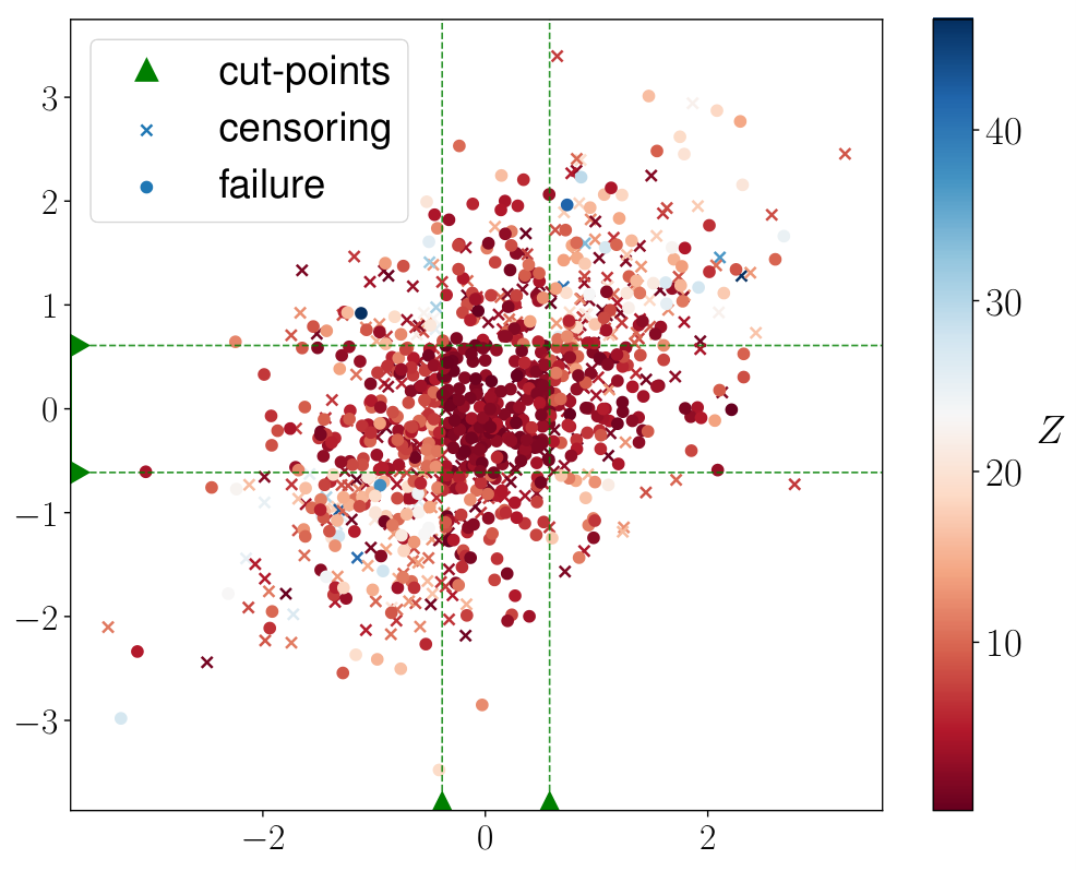
with ν>0\nu>0 and ς>0\varsigma>0 the scale and shape parameters respectively, and Ui∼𝒰⁡([0,1])U_{i}\sim\mathcal{U}([0,1]), where 𝒰⁡([a,b])\mathcal{U}([a,b]) stands for the uniform distribution on a segment [a,b][a,b]. The distribution of the censoring variable CiC_{i} is the geometric distribution 𝒢⁡(αc)\mathcal{G}(\alpha_{c}), where αc∈(0,1)\alpha_{c}\in(0,1) is empirically tuned to maintain a desired censoring rate rc∈[0,1]r_{c}\in[0,1]. The choice of all hyper-parameters is driven by the applications on real data presented in Section 5, and summarized in Table 1. Figure 3 gives an example of data generated according to the design we have just described.

Table 1: Hyper-parameter choices for simulation.
nn pp ρ\rho Kj⋆K^{\star}_{j} ν\nu ς\varsigma rcr_{c} rsr_{s}
(200, 4000) 50 0.5 {1,2,3}\{1,2,3\} 2 0.1 0.3 0.2
Fig. 3: Left: illustration of data simulated with p=2p=2, K1⋆=K2⋆=2K^{\star}_{1}=K^{\star}_{2}=2, and n=1000n=1000. Dots represent failure times (zi=ti)(z_{i}=t_{i}) while crosses represent censoring times (zi=ci)(z_{i}=c_{i}), and the colour gradient represents the ziz_{i} values (red for low and blue for high). Right: β⋆\beta^{\star} is plotted, with a dotted line to demarcate the two blocks (since p=2p=2).
Refer to caption

4.2.2 Metrics.

We evaluate the methods being analysed using two metrics. The first assesses the estimation of the cut-points values by

m1=|𝒮′|−1​∑j∈𝒮′ℋ⁡(ℳj⋆,ℳ^j),m_{1}=|\mathcal{S}^{\prime}|^{-1}\sum_{j\in\mathcal{S}^{\prime}}\ \mathcal{H}(\mathcal{M}^{\star}_{j},\widehat{\mathcal{M}}_{j}),

where ℳj⋆={μj,1⋆,…,μj,Kj⋆⋆}\mathcal{M}^{\star}_{j}=\{\mu^{\star}_{j,1},\ldots,\mu^{\star}_{j,K^{\star}_{j}}\} (resp. ℳ^j={μ^j,1,…,μ^j,K^j}\widehat{\mathcal{M}}_{j}=\{\hat{\mu}_{j,1},\ldots,\hat{\mu}_{j,\widehat{K}_{j}}\}) is the set of true (resp. estimated) cut-points for feature jj,  𝒮′={j,j∉𝒮∩{l,ℳ^l=∅}}\mathcal{S}^{\prime}=\big\{j,\ j\notin\mathcal{S}\cap\{l,\ \widehat{\mathcal{M}}_{l}=\emptyset\}\big\} the indexes corresponding to features with at least one true cut-point and one detected cut-point, and ℋ⁡(A,B)\mathcal{H}(A,B) the Hausdorff distance between the sets AA and BB, defined as

ℋ(A,B)=max(ℰ(A||B),ℰ(B||A)),\mathcal{H}(A,B)=\max\big(\mathcal{E}(A||B),\mathcal{E}(B||A)\big),

where ℰ(A||B)=supb∈Binfa∈A|a−b|\mathcal{E}(A||B)=\sup_{b\in B}\inf_{a\in A}|a-b|. This is inspired by Harchaoui and Lévy-Leduc (2010), except that in our case, both ℳj⋆\mathcal{M}^{\star}_{j} and ℳ^j\widehat{\mathcal{M}}_{j} can be empty, which explains the use of 𝒮′\mathcal{S}^{\prime}. The second metric we use is precisely focused on the sparsity aspect; it assesses the ability for each method to detect features with no cut-points, and is defined by

m2=|𝒮|−1​∑j∈𝒮K^j.m_{2}=|\mathcal{S}|^{-1}\sum_{j\in\mathcal{S}}\widehat{K}_{j}.

4.3 Competing methods

To the best of our knowledge, all existing algorithms and methods are based on multiple log-rank tests in univariate models. These methods are widely used, and recent implementations include the web applications Cutoff Finder and Findcutoffs described in Budczies et al. (2012) and Chang et al. (2017) respectively.

We describe in what follows the principle of these univariate log-rank tests. Consider one of the initial variables 𝑿∙,j=(x1,j,…,xn,j)⊤\boldsymbol{X}_{\bullet,j}=(x_{1,j},\ldots,x_{n,j})^{\top}, and denote its 10th and 90th quantiles as x10​t​h,jx_{10th,j} and x90​t​h,jx_{90th,j}. Then, define a grid {gj,1,…,gj,κj}\{g_{j,1},\ldots,g_{j,\kappa_{j}}\}. In most implementations, the gj,kg_{j,k}’s are chosen at the original observation points and are such that x10​t​h,j≤gj,k≤x90​t​h,jx_{10th,j}\leq g_{j,k}\leq x_{90th,j}. For each gj,kg_{j,k}, the pp-value pvj,k\text{pv}_{j,k} of the log-rank test associated with the univariate Cox model defined by

λ0​(t)​exp⁡(βj​𝟙​(x≤gj,k))\lambda_{0}(t)\exp\big(\beta^{j}\mathds{1}(x\leq g_{j,k})\big)

is computed (via the python package lifelines in our implementation). For each initial variable 𝑿∙,j\boldsymbol{X}_{\bullet,j}, κj\kappa_{j} pp-values are available at this stage. The choice of the size κj\kappa_{j} of the grid depends on the implementation, and ranges for several dozen to all observed values between x10​t​h,jx_{10th,j} and x90​t​h,jx_{90th,j}.

In Figure 4, the values −log⁡(pvj,k)-\log(\text{pv}_{j,k}) for k=1,…,κjk=1,\ldots,\kappa_{j} (denoted by “MT” for “Multiple Testing”) are represented, for the simulated example illustrated in Figure 3. Notice that the level −log⁡(α)=−log⁡(0.05)-\log(\alpha)=-\log(0.05) is exceeded for numerous gj,kg_{j,k}’s values, and of course this procedure allows us to detect only a single cut-point per feature. A common approach is to consider the maximal value −log⁡(pvj,k^)-\log(\text{pv}_{j,\hat{k}}) and then define the cut-point for variable jj as gj,k^g_{j,\hat{k}}. As argued in Altman et al. (1994), this is obviously “associated with an inflation of type I error”, and for this reason we do not consider this approach.

To cope with the multiple testing (MT) problem at hand, multiple testing corrections have to be applied, of which we consider two. The first is the well-known Bonferroni pp-value correction, referred to as MT-B in the following. We insist on the fact that although commonly used, this method is not correct in this situation since the pp-values are correlated. Note also that in this context, the Benjamini–Hochberg (BH) procedure would result in the same cut-points being detected as MT-B (with FDR=α\alpha), since we only consider as a cut-point candidate the points with minimal pp-value. Indeed, applying the classical BH procedure would select far too many cut-points. The second correction, denoted MT-LS, is the correction proposed in Lausen and Schumacher (1992), based on asymptotic theoretical considerations. Figure 4 also illustrates how these corrections behave on the simulated example illustrated in Figure 3. A third correction we could imagine would be a bootstrap-based MaxT procedure (or MinP) as proposed in Dudoit and Van Der Laan (2007) or Westfall et al. (1993), but this would be intractable in our high-dimensional setting (see Figure 5(a) that compares the computing times for a single feature only; a bootstrap procedure based on MT would dramatically increase the required computing time).

4.4 Simulation results

4.4.1 Example.

Figure 4 illustrates how the methods considered behave on the data shown in Figure 3. With the help of this example, we can clearly see the good performance of the binacox method: the position, strength and number of cut-points are well estimated. The MT-B and MT-LS methods can only detect one cut-point by construction. Both methods detect “the most significant” cut-point for each of the 2 features, namely those corresponding to the highest jumps in βj,∙⋆\beta^{\star}_{j,\bullet} (see Figure 3): μ1,1⋆\mu^{\star}_{1,1} and μ2,2⋆\mu^{\star}_{2,2}.

With regards to the shape of the “pp-value curves”, one can see that for each of the two features, the two “main” local maxima correspond to the true cut-points. One could then imagine creating a method for detecting such maxima, but this is beyond the scope of this paper (plus it would still be based on MT methods, which have high computational costs, as detailed hereafter).

Fig. 4: Top: Illustration of the main quantities involved in the binacox, with estimations obtained for the data represented in Figure 3. Our algorithm detects the correct number of cut-points K^j=2\widehat{K}_{j}=2, and estimates their positions accurately, as well as their amplitudes. Bottom: results obtained using the multiple testing-related methods introduced in Section 4.3. Here the BH threshold lines overlap that corresponding to α=5%\alpha=5\%. The BH procedure would consider as cut-points all μj,l\mu_{j,l} values for which the corresponding dark green (MT) line’s values are above this, thus detecting far too many cut-points.

4.4.2 Computing times.

Now let us look at the computing time required for the methods considered. As the multiple testing-related methods are univariate, we can directly parallelize their computations across dimensions (which is what we did in the applications), so let us consider here a single feature XX (p=1p=1). Following the method explained in Section 4.3, we have to compute all log-rank test pp-values computed on the populations {yi:xi>μ}\{y_{i}:x_{i}>\mu\} and {yi:xi≤μ}\{y_{i}:x_{i}\leq\mu\} for i=1,…,ni=1,\ldots,n, for μ\mu taking all xix_{i} values between the 10th and 90th empirical quantiles of XX. We denote “MT all” this method in Figure 5(a), and compare its computing times with the binacox for various values of nn. We also show the “MT grid” method that only computes the pp-values for candidates μj,l\mu_{j,l} used in the binacox method.

Since the number of candidates does not change with nn for the “MT grid” method, the computing time ratio between “MT all” and “MT grid” naturally increases, going roughly from one to two orders of magnitude higher when nn goes from 300 to 4000. Hence to make computations much faster, we will use the “MT grid” for all multiple testing-related methods in the following. The resulting loss of precision in the MT-related methods is negligible for a high enough djd_{j} (=50=50 in practice).

Next, we emphasize the fact that the binacox is still roughly 5 times faster than the “MT grid” method, and it remains very fast when we increase the dimension, as shown in Figure 5(b). It turns out that the computational time grows roughly logarithmically with pp.

(a) Average computing times in seconds (with the black lines representing ±\pm the standard deviation) obtained on 100 simulated datasets (according to Section 4.2 with p=1p=1 and K⋆=2K^{\star}=2) for training the binacox versus the multiple testing methods, where cut-point candidates are either all xix_{i} values between the 10th and 90th empirical quantiles of XX (“MT all”), or the same candidates as the grid considered by the binacox (“MT grid”).
(b) Average (bold) computing times in seconds and standard deviation (bands) obtained on 100 simulated datasets (according to Section 4.2 with Kj⋆=2K^{\star}_{j}=2) for training the binacox when increasing the dimension pp up to 100. The method remains very fast in high-dimensional settings.
Fig. 5: Computing time for the methods considered.

4.4.3 Performance comparison.

Let us compare now the results of simulations in terms of the m1m_{1} and m2m_{2} metrics introduced in Section 4.2. Figure 6 gives a comparison of the methods considered for the cut-point estimation aspect, i.e., in terms of the m1m_{1} score. It appears that the binacox outperforms the MT-related methods when Kj⋆>1K^{\star}_{j}>1, and is competitive when Kj⋆=1K^{\star}_{j}=1 except for small values of nn. This is due to an overestimation in the number of cut-points by the binacox (see Figure 7), especially when pp is high and nn is small, which gives higher m1m_{1} values, even if the “true” cut-point is actually well-estimated. Note that for such values of pp, the binacox runs much faster than the MT-related methods.

Fig. 6: Average (bold) m1m_{1} scores and standard deviation (bands) obtained on 100 datasets simulated according to Section 4.2 with p=50p=50 and Kj⋆K^{\star}_{j} equal to 1, 2 and 3 (for all j=1,…,pj=1,\ldots,p) for the left, center and right sub-figures respectively) for varying nn. The lower the value of m1m_{1}, the better the result; the binacox clearly outperforms the other methods when there is more than one cut-point, and is competitive with other methods when there is only one cut-point, but performs worse when nn is small because it overestimates Kj⋆K^{\star}_{j}.

Figure 7, on the other hand, assesses the ability of each method to detect features with no cut-points using the m2m_{2} metric, i.e., the ability to estimate K^j⋆=0\hat{K}^{\star}_{j}=0 for j∈𝒮j\in\mathcal{S}. The binacox appears to be quite effective at detecting features with no cut-point when nn takes a high enough value compared to pp, which is not the case for the MT-related methods.

Fig. 7: Average (bold) m2m_{2} scores and standard deviation (bands) obtained on 100 datasets simulated according to Section 4.2 with p=50p=50 for varying nn. MT-B and MT-LS tend to detect a cut-point when there is none (no matter the value of nn), while binacox overestimates the number of cut-points for small values of nn but detects 𝒮\mathcal{S} well for p=50p=50 on the simulated data when n>1000n>1000.

5 Application on genetic data

In this section, we apply our method to three biomedical datasets. We extracted normalized expression data and survival times ZZ in days from breast invasive carcinoma (BRCA, n=1211n=1211), glioblastoma multiforme (GBM, n=168n=168) and kidney renal clear cell carcinoma (KIRC, n=605n=605). These datasets are available on The Cancer Genome Atlas (TCGA) platform, which aims to accelerate the understanding of the molecular basis of cancer with the help of genomic technology, including large-scale genome sequencing. For each patient, 20,531 features corresponding to normalized gene expression values are available.

As we saw in Section 4.4, the MT-related methods are intractable in such high-dimensional cases. We therefore include a screening step to select the portion of features most relevant to our problem from the 20,531 available. To do so, we fit the binacox on each jjth block separately and take the resulting ‖β^j,∙‖TV\|\hat{\beta}_{j,\bullet}\|_{\TV} as a score that roughly assess the propensity for feature jj to have one (or more) relevant cut-point(s). We then select the features corresponding to the top PP values with P=50P=50, this choice being suggested by the distribution of the obtained scores given in Figure 12 of Appendix A.3.

5.1 Estimation results.

In Figure 8 we present the results obtained by the methods considered on the GBM cancer dataset for the top 10 features ordered according to the binacox ‖β^j,∙‖TV\|\hat{\beta}_{j,\bullet}\|_{\TV} values. We observe that all cut-points detected by the univariate multiple testing methods with Bonferroni (MT-B) or Lausen and Schumacher (MT-LS) corrections are also detected by the multivariate binacox (which detects more cut-points); see Table 2. The binacox identifies many more cut-points than the univariate MT-B and MT-LS methods. Further, all cut-points detected by these two methods are also detected by the binacox. Furthermore, it turns out that these top 10 genes (from the original 20,531) are quite relevant to GBM, the most aggressive cancer that begins in the brain.

For instance, the first gene, SOD3, is relevant from a physiopathological point of view since its polymorphisms are already known as GBM risk factors (Rajaraman et al., 2008). Other genes in the top 10 (C11orf63 or the HOX genes) are also known to be directly related to brain development (Canu et al., 2009), and are already known as potential GBM prognosis marker (Duan et al., 2015; Guan et al., 2019).

Table 2: Estimated cut-point values for each method on the top 10 genes presented in Figure 8 for GBM. Dots (⋅\cdot) mean “no cut-point detected”.
Genes Binacox MT-B MT-LS
SOD3 6649 200.87, 326.40, 606.48 ⋅\cdot ⋅\cdot
LOC 400752 31.46, 62.50 ⋅\cdot 34.04
C11orf63 79864 40.30, 109.67 19.65 19.65
KTI12 112970 219.60, 305.70 219.60 219.60
HOXC8 3224 3.30, 15.75 3.30 3.30
DDX5 1655 10630.11, 13094.89 ⋅\cdot ⋅\cdot
FKBP9L 360132 111.72 ⋅\cdot ⋅\cdot
HOXA1 3198 67.28 ⋅\cdot ⋅\cdot
MOSC2 54996 107.53 107.53 107.53
ZNF680 340252 385.85, 638.06 385.85 385.85
Fig. 8: Illustration of the results obtained on the top 10 features ordered according to the binacox ‖β^j,∙‖TV\|\hat{\beta}_{j,\bullet}\|_{\TV} values on the GBM dataset. The binacox detects multiple cut-points and sheds light on non-linear effects for various genes. The BH thresholds are shown, but are unusable in practice.

Relevant results were also obtained on the KIRC and BRCA datasets; these are postponed to Appendix A.4.

5.2 Risk prediction.

Let us now investigate how performances are impacted in terms of risk prediction when detected cut-points are taken into account; namely, comparing predictions when training a Cox model on the original continuous feature space versus on the μ^\widehat{\mu}-binarized space constructed with the cut-point estimates.

In a classical Cox model, Ri=exp⁡(Xi⊤​β^)R_{i}=\exp(X_{i}^{\top}\hat{\beta}) is known as the predicted risk for patient ii measured at t=0t=0. A common metric to evaluate risk prediction performances in this type of survival setting is the C-index (Heagerty and Zheng, 2005), which is defined by

𝒞τ=ℙ[Ri>Rj|Zi<Zj,Zi<τ],\mathcal{C}_{\tau}=\mathbb{P}[R_{i}>R_{j}|Z_{i}<Z_{j},Z_{i}<\tau],

with i≠ji\neq j two independent patients and τ\tau the follow-up period. A Kaplan-Meier estimator for the censoring distribution leads to a nonparametric and consistent estimator of 𝒞τ\mathcal{C}_{\tau} (Uno et al., 2011), which is already implemented in the python package lifelines.

We randomly split the three datasets 100 times into training and validation sets (30% for testing) and compare the average C-index on the validation sets in Table 3 when the μ^\widehat{\mu}-binarized space is constructed based on the μ^\widehat{\mu}’s obtained either from the binacox, MT-B, or MT-LS. We also compare performances obtained by two nonlinear multivariate methods known to perform well in high-dimensional settings: boosted Cox (CoxBoost) (Li and Luan, 2005) used with 300 boosting steps (this number being fine-tuned by cross-validation), and random survival forests (RSF) (Ishwaran et al., 2008) used with 200 trees (also cross-validated), respectively implemented in the R packages CoxBoost and randomForestSRC. Note that for a fair comparison, and to avoid selection bias (Ambroise and McLachlan, 2002), the screening step is re-run on each training set, using the C-index obtained by univariate Cox models (not to confer advantage to our method), namely Cox PH models fitted on each covariate separately.

Table 3: Comparison of average C-indexes (and standard deviation in parentheses) on 100 random train/test splits for the Cox model trained on continuous features versus on its binarized version constructed using the considered methods’ cut-point estimates, and the CoxBoost and RSF methods. On the three datasets, the binacox method gives by far the best results (in bold).
Cancer Continuous Binacox MT-B MT-LS CoxBoost RSF
GBM 0.563 (0.037) 0.603 (0.048) 0.579 (0.049) 0.577 (0.043) 0.569 (0.037) 0.564 (0.036)
KIRC 0.675 (0.028) 0.709 (0.022) 0.682 (0.022) 0.682 (0.022) 0.683 (0.029) 0.695 (0.026)
BRCA 0.592 (0.050) 0.669 (0.047) 0.626 (0.055) 0.621 (0.061) 0.598 (0.053) 0.659 (0.037)
Fig. 9: Average computing times (in seconds) required by each method on the three datasets (with the black lines representing ±\pm the standard deviation) obtained on 100 random train/test split. The binacox method is at least one and up to several orders of magnitude faster.

The binacox method clearly improves risk prediction compare to classical Cox, as well as with respect to the MT-B and MT-LS methods. Moreover, it also significantly outperforms both CoxBoost and RSF. To the best of our knowledge, no better performances have been achieved on this data in the literature (Yousefi et al., 2017). Figure 9 compares the computing times of the methods. Clearly the binacox is by far the most computationally efficient.

6 Conclusion

In this paper, we introduced the binacox method, designed for estimating multiple cut-points in a Cox model with high-dimensional features. We illustrated the good theoretical properties of the model by establishing nonasymptotic oracle inequalities for prediction and estimation. An extensive Monte Carlo simulation study was then carried out to evaluate the method’s performance. It showed that our approach outperforms existing methods, with computing times orders of magnitude faster. Moreover, in addition to the raw feature selection ability of the binacox, it succeeds in detecting multiple cut-points per feature. We also applied the binacox to three publicly available high-dimensional genetics datasets. Furthermore, several genes pinpointed by the model turn out to be biologically relevant (e.g., the gene SOD3 for GBM), whilst others require further investigation in the genetics research community. More importantly, our method provides powerful interpretation aspects that could be useful in both clinical research and daily practice. Indeed, the estimated cut-points could be directly considered in clinical practice. Thus, the method could be an interesting alternative to more classical methods found in the medical literature to deal with prognosis studies in high-dimensional frameworks, providing a new way to model nonlinear feature associations, and giving rise to new data-driven risk scores. Our study lays the groundwork for the development of powerful methods which could one day help provide improved personalized care.

Acknowledgments

Mokhtar Z. Alaya is grateful for a grant from DIM Math Innov Région Ile-de-France http://www.dim-mathinnov.fr. Agathe Guilloux’s work has been supported by the INCA-DGOS grant PTR-K 2014. The results shown in this paper are based upon data generated by the TCGA Research Network and freely available from http://cancergenome.nih.gov. Conflict of Interest: None declared.

Software

All methodology discussed in the paper is implemented in Python/C++ and R. The code that generates all figures is available from https://github.com/SimonBussy/binacox in the form of annotated programs, together with notebook tutorials.

Appendix A Additional details

A.1 Algorithm.

To solve regularization problem (5), we first look at the proximal operator of the binarsity penalty (Alaya et al., 2017). It turns out that it can be computed very efficiently, using an algorithm introduced in Condat (2013) that we modify in order to include the weights ωj,k\omega_{j,k}. It basically applies – in each block – the proximal operator of the total variation (since the binarsity penalty is block separable), followed by a centering within each block to satisfy the constraint, see Algorithm 1 below. We refer to Alaya et al. (2015) for the weighted total variation proximal operator.

Algorithm 1 Proximal operator of bina⁡(β)\bina(\beta), see (Alaya et al., 2017)
 Input: vector β∈ℬp+d​(R)\beta\in\mathscr{B}_{p+d}(R) and weights ωj,l\omega_{j,l} for j=1,…,pj=1,\ldots,p and l=1,…,dj+1l=1,\ldots,d_{j}+1
 Output: vector η={prox}bina⁡(β)\eta=\prox_{\bina}(\beta)
 for j=1j=1 to pp do
  θj,∙←{prox}∥⋅∥TV,ωj,∙(βj,∙)\theta_{j,\bullet}\leftarrow\prox_{\|\cdot\|_{\TV,\omega_{j,\bullet}}}(\beta_{j,\bullet}) (TV-weighted in block jj, see (7))
  ηj,∙←θj,∙−nj,∙⊤​θj,∙‖nj,∙‖22​nj,∙\eta_{j,\bullet}\leftarrow\theta_{j,\bullet}-\frac{n_{j,\bullet}^{\top}\theta_{j,\bullet}}{\|n_{j,\bullet}\|_{2}^{2}}n_{j,\bullet} (projection onto span​(nj,∙)⟂\text{span}(n_{j,\bullet})^{\perp})
 end for
 Return: η\eta

A.2 Implementation

Figure 10 gives the learning curves obtained during the VV-fold cross-validation procedure presented in Section 4.3 with V=10V=10 for the fine-tuning of parameter γ\gamma, which is the strength of the binarsity penalty. We randomly split the data into training and validation sets (30% for validation, cross-validation being done on the training). Recall that the score we use is the negative partial log-likelihood defined in (4) computed after a refit of the model on the binary space obtained by the estimated cut-points, with the sum-to-zero constraint in each block but without the TV penalty.

Fig. 10: Learning curves obtained for various γ\gamma, in blue on the different test sets during cross-validation, and in orange on the validation set. Bold lines represent average scores on the folds, and bands represent 95% Gaussian confidence intervals. The green triangle points out the value of γ−1\gamma^{-1} that gives the minimum score (best training score), while the γ−1\gamma^{-1} value we automatically select (the red triangle) is the smallest value such that the score is within one standard error of the minimum, which is a classical trick (Simon et al., 2011) that favors a slightly higher penalty strength (smaller γ−1\gamma^{-1}) to avoid over-estimation of K⋆K^{\star} in our case.

Figure 11 illustrates the de-noising step for the cut-point detection when looking at the β^\hat{\beta} support relative to the TV norm. The β^\hat{\beta} vector plotted here corresponds to the data generated in Figure 3 of Section 4.2, where the final estimation results were presented in Figure 4 of Section 4.4. Since it is usual to observe three consecutive β^\hat{\beta}’s jumps in the neighbourhood of a true cut-point, which is the case in Figure 11 for the first and the last jumps, this could lead to an over-estimation of K⋆K^{\star}. To bypass this problem, we then use the following rule: if β^\hat{\beta} has three consecutive different coefficients within a block, then only the largest jump is considered as a “true” one.

Fig. 11: Illustration of the de-noising step in the cut-point detection phase on the simulated date of Figure 3. Within each block (separated with the dotted pink line), the different colors represent β^j,l\hat{\beta}_{j,l} with corresponding μj,l\mu_{j,l} in distinct estimated Ij,k⋆I^{\star}_{j,k}. The following rule is applied: when a β^j,l\hat{\beta}_{j,l} is “isolated”, it is assigned to its “closest” group.

A.3 TCGA gene screening

Figure 12 illustrates the screening procedure followed to reduce the high-dimensionality of the TCGA datasets to make the multiple testing related methods tractable. We then fit a univariate binacox on each block jj separately and compute the resulting ‖β^j,∙‖TV\|\hat{\beta}_{j,\bullet}\|_{\TV} to assess the propensity for feature jj to obtain one (or more) relevant cut-point(s). It appears that taking the top PP features with P=50P=50 is a reasonable choice for each dataset considered.

Fig. 12: ‖β^j,∙‖TV\|\hat{\beta}_{j,\bullet}\|_{\TV} obtained for univariate binacox fits for the three datasets considered. The top PP selected features appear in red, and it turns out that taking P=50P=50 coincides with the elbow (represented with the dotted grey lines) in each of the three curves.

A.4 Results on BRCA and KIRC data

Figure 13 illustrates the results obtained by all methods we consider on the BRCA cancer dataset for the top 10 features ordered according to the binacox ‖β^j,∙‖TV\|\hat{\beta}_{j,\bullet}\|_{\TV} values. Table 4 summarizes the detected cut-point values for each method. It turns out that the selected genes are quite relevant from a clinical point of view (for instance, NPRL2 is a tumor suppressor gene (Huang et al., 2016)), and in particular for BRCA (breast) cancer. For instance, HBS1L expression is known for being predictive of breast cancer survival (Antonov et al., 2014; Antonov, 2011; BioProfiling, 2009), while FOXA1 and PPFIA1 are highly related to breast cancer, see Badve et al. (2007) and Dancau et al. (2010) respectively.

Fig. 13: Illustration of the results obtained on the top 10 features ordered according to the binacox ‖β^j,∙‖TV\|\hat{\beta}_{j,\bullet}\|_{\TV} values on the BRCA dataset.
Table 4: Estimated cut-point values for each method on the top 10 genes presented in Figure 13 for BRCA.
Genes Binacox MT-B MT-LS
PLCH2 9651 28.43, 200.74, 273.04, 382.87 382.87 382.87
NPRL2 10641 330.64, 568.06 330.64 330.64
HBS1L 10767 1023.91, 1212.54, 1782.77 1782.77 1782.77
FGD4 121512 163.59, 309.24 517.90 517.90
MEA1 4201 2199.21 786.29 786.29
ARHGAP39 80728 493.01, 734.37, 1049.04 265.26 265.26
FOXA1 3169 11442.32 3586.03 3586.03
PPFIA1 8500 1500.02, 1885.27 1152.98 1152.98
PRCC 5546 2091.16, 2194.08 1165.49 1165.49
PGK1 5230 10205.72, 12036.29 12036.29 12036.29

Lastly, Figure 14 gives the results obtained by the various methods on the KIRC cancer dataset for the top 10 features ordered according to the binacox ‖β^j,∙‖TV\|\hat{\beta}_{j,\bullet}\|_{\TV} values, and Table 5 summarizes the detected cut-point values for each method. Once again, the selected genes are relevant for cancer studies including KIRC. For instance, EIF4EBP2 is related to cancer proliferation (Mizutani et al., 2016)), RGS17 is known to be overexpressed in various cancers (James et al., 2009), and both COL7A1 and NUF2 are known to be related to renal cell carcinoma (see (Csikos et al., 2003) and (Kulkarni et al., 2012) respectively). Moreover, the first two genes MARS 4141 and STRADA 92335 already appear as relevant KIRC prognosis markers in Bussy et al. (2019) .

Fig. 14: Illustration of the results obtained on the top 10 features ordered according to the binacox ‖β^j,∙‖TV\|\hat{\beta}_{j,\bullet}\|_{\TV} values on the KIRC dataset.
Table 5: Estimated cut-point values for each method on the top 10 genes illustrated in Figure 14 for KIRC.
Genes Binacox MT-B MT-LS
MARS 4141 1196.21, 1350.00 1350.00 1350.00
STRADA 92335 495.24, 553.73 586.88 586.88
PTPRH 5794 3.32 3.32 3.32
EIF4EBP2 1979 6504.80 5455.59 5455.59
RGS17 26575 4.30 4.30 4.30
COL7A1 1294 44.19 113.08 113.08
HJURP 55355 99.83 134.31 134.31
NUF2 83540 42.18 63.09 63.09
NDC80 10403 91.39 107.53 107.53
CDCA3 83461 52.03 110.18 110.18

Appendix B Proof of Theorem 1

In this section, we provide the proof of Theorem 1. First, we derive some preliminary results which will be required in the following.

B.1 Preliminary results

Additional notation.

For u,v∈ℝmu,v\in{\mathbb{R}}^{m}, we denote by u⊙vu\odot v the Hadamard product defined by u⊙v=(u1​v1,…,um​vm)⊤.u\odot v=(u_{1}v_{1},\ldots,u_{m}v_{m})^{\top}. We denote by sign⁡(u)\sgn(u) the subdifferential of the function u↦|u|u\mapsto|u|, i.e.,

sign⁡(u)={{1} if ​u>0,[−1,1] if ​u=0,{−1} if ​u<0.\sgn(u)=\begin{cases}\{1\}&\text{ if }u>0,\\ [-1,1]&\text{ if }u=0,\\ \{-1\}&\text{ if }u<0.\end{cases}

We write ∂(ϕ)\partial(\phi) for the subdifferential mapping of a convex functional ϕ\phi. We adopt in the proofs counting process notation. We then define the observed-failure counting process Ni​(t)=𝟙​(Zi≤t,Δi=1),N_{i}(t)=\mathds{1}(Z_{i}\leq t,\Delta_{i}=1), the at-risk process Yi​(t)=𝟙​(Zi≥t),Y_{i}(t)=\mathds{1}(Z_{i}\geq t), and N¯​(t)=1n​∑i=1nNi​(t).\bar{N}(t)=\dfrac{1}{n}\sum_{i=1}^{n}N_{i}(t). For every vector vv, let us denote v⊗0=1v^{\otimes 0}=1, v⊗1=v,v^{\otimes 1}=v, and v⊗2=v​v⊤v^{\otimes 2}=vv^{\top} (outer product). Recall finally that τ>0\tau>0 denotes the finite study duration.

Weights.

For a given numerical constant c>0c>0, the weights ωj,l\omega_{j,l} have an explicit form given by

ωj,l=5.64​c+log⁡(p+d)+ℒn,cn+18.62​(c+log⁡(p+d)+1+ℒn,c)n,\omega_{j,l}=5.64\sqrt{\frac{c+\log(p+d)+\mathscr{L}_{n,c}}{n}}+18.62\frac{(c+\log(p+d)+1+\mathscr{L}_{n,c})}{n}, (20)

where ℒn,c=2​log⁡log⁡((2​e​n+24​e​c)∨e)\mathscr{L}_{n,c}=2\log\log\big((2en+24ec)\vee e\big).

Properties of the binarsity penalty.

We define ω=(ω1,∙,…,ωp,∙)\omega=(\omega_{1,\bullet},\ldots,\omega_{p,\bullet}) the weights vector, with ωj,1=0\omega_{j,1}=0 for all j=1,…,pj=1,\ldots,p. Then, we rewrite the total variation part in the binarsity penalty as follows. Let us define the (dj+1)×(dj+1)(d_{j}+1)\times(d_{j}+1) matrix DjD_{j} by

Dj=[100−11⋱⋱0−11]∈ℝdj+1×ℝdj+1.{D}_{j}=\begin{bmatrix}1&0&&0\\ -1&1&\\ &\ddots&\ddots\\ 0&&-1&1\end{bmatrix}\in{\mathbb{R}}^{d_{j}+1}\times{\mathbb{R}}^{d_{j}+1}.

We then remark that for all βj,∙∈ℝdj+1\beta_{j,\bullet}\in{\mathbb{R}}^{d_{j}+1}, one has ‖βj,∙‖TV,ωj,∙=‖ωj,∙⊙Dj​βj,∙‖1\|\beta_{j,\bullet}\|_{\TV,\omega_{j,\bullet}}=\|\omega_{j,\bullet}\odot{D}_{j}\beta_{j,\bullet}\|_{1}. Moreover, note that the matrix Dj{D}_{j} is invertible. We denote its inverse Tj{{T}_{j}}, which is defined by the (dj+1)×(dj+1)(d_{j}+1)\times(d_{j}+1) lower triangular matrix with entries (Tj)r,s=0({{T}_{j}})_{r,s}=0 if r<sr<s and (Tj)r,s=1({{T}_{j}})_{r,s}=1 otherwise. We set

𝐃=diag⁡(D1,…,Dp) and 𝐓=diag⁡(T1,…,Tp).{{\bf{D}}}=\diag({D}_{{1}},\ldots,{D}_{{p}})\quad\textrm{ and }\quad{{\bf{T}}}=\diag({T}_{{1}},\ldots,{T}_{{p}}). (21)

Lemma 1 then states that binarsity is a sub-additive penalty (Kutateladze, 2013).

Lemma 1

For all β,β′∈ℝp+d\beta,\beta^{\prime}\in{\mathbb{R}}^{p+d}, we have that

bina⁡(β+β′)≤bina⁡(β)+bina⁡(β′)andbina⁡(−β)≤bina⁡(β).\bina(\beta+\beta^{\prime})\leq\bina(\beta)+\bina(\beta^{\prime})\quad\text{and}\quad\bina(-\beta)\leq\bina(\beta).

Proof of Lemma 1. The hyperplane span​{u∈ℝdj+1:nj,∙⊤​u=0}\text{span}\{u\in{\mathbb{R}}^{d_{j}+1}:n_{j,\bullet}^{\top}u=0\} is a convex cone, then the indicator function δj\delta_{j} is sublinear (i.e., positively homogeneous and sub-additive (Kutateladze, 2013)). Furthermore, the total variation penalization satisfies the triangle inequality, which gives the first statement of Lemma 1. To prove the second, we use the fact that δj​(βj,∙)+δj​(−βj,∙)≥0\delta_{j}(\beta_{j,\bullet})+\delta_{j}(-\beta_{j,\bullet})\geq 0 to obtain:

bina⁡(−β)OPEN=∑j=1p(‖βj,∙‖TV,ωj,∙+δj​(−βj,∙))≤∑j=1p(‖βj,∙‖TV,ωj,∙+δj​(βj,∙)))=bina⁡(β),\begin{split}\bina(-\beta)&=\sum_{j=1}^{p}\Big(\|\beta_{j,\bullet}\|_{\TV,\omega_{j,\bullet}}+\delta_{j}(-\beta_{j,\bullet})\Big)\leq\sum_{j=1}^{p}\Big(\|\beta_{j,\bullet}\|_{\TV,\omega_{j,\bullet}}+\delta_{j}(\beta_{j,\bullet}))\Big)=\bina(\beta),\end{split}

which concludes the proof of Lemma 1. □\hfill\square

Additional useful quantities.

The Doob-Meyer decomposition (Aalen, 1978) implies that, for all i=1,…,ni=1,\ldots,n and all t≥0t\geq 0,

d​Ni​(t)=Yi​(t)​λ0⋆​(t)​ef⋆​(Xi)​d​t+d​Mi​(t),\mathrm{d}N_{i}(t)=Y_{i}(t)\lambda_{0}^{\star}(t)e^{f^{\star}(X_{i})}\mathrm{d}t+\mathrm{d}M_{i}(t),

where the martingales MiM_{i} are square integrable and orthogonal. With this notation, we define, for all t≥0t\geq 0 and any ff, the process

Sn(r)​(f,t)=∑i=1nYi​(t)​ef⁡(Xi)​(XiB)⊗rS_{n}^{(r)}(f,t)=\sum_{i=1}^{n}Y_{i}(t)e^{f(X_{i})}(X_{i}^{B})^{\otimes r}

for r∈{0,1,2}r\in\{0,1,2\}, where XiBX_{i}^{B} is the iith row of the binarized matrix 𝑿B\boldsymbol{X}^{B}. The empirical loss ℓn\ell_{n} can then be rewritten as

ℓn(f)=−1n∑i=1n∫0τ{f(Xi)−log(Sn(0)(f,t))}dNi(t).\displaystyle\ell_{n}(f)=-\frac{1}{n}\sum_{i=1}^{n}\int_{0}^{\tau}\big\{f(X_{i})-\log\big(S_{n}^{(0)}(f,t)\big)\big\}\mathrm{d}N_{i}(t).

Together with this loss, we introduce the loss

ℓ⁡(f)\displaystyle\ell(f) =−1n∑i=1n∫0τ{f(Xi)−log(Sn(0)(f,t))}Yi(t)λ0⋆(t)ef⋆​(Xi)dt\displaystyle=-\frac{1}{n}\sum_{i=1}^{n}\int_{0}^{\tau}\big\{f(X_{i})-\log\big(S_{n}^{(0)}(f,t)\big)\big\}Y_{i}(t)\lambda_{0}^{\star}(t)e^{f^{\star}(X_{i})}\mathrm{d}t
=−1n∑i=1n∫0τlog(ef⁡(Xi)Sn(0)​(f,t))Yi(t)λ0⋆(t)ef⋆​(Xi)dt.\displaystyle=-\frac{1}{n}\sum_{i=1}^{n}\int_{0}^{\tau}\log\Big(\dfrac{e^{f(X_{i})}}{S_{n}^{(0)}(f,t)}\Big)Y_{i}(t)\lambda_{0}^{\star}(t)e^{f^{\star}(X_{i})}\mathrm{d}t.

We will use the fact that for a function fβf_{\beta} of the form fβ​(Xi)=β⊤​XiB=∑j=1pfβj,∙​(Xi)f_{\beta}(X_{i})=\beta^{\top}{X_{i}^{B}}=\sum_{j=1}^{p}f_{\beta_{j,\bullet}}(X_{i}), the Doob-Meyer decomposition implies that

∇ℓn​(fβ)\displaystyle\nabla\ell_{n}(f_{\beta}) =−1n∑i=1n∫0τ{XiB−Sn(1)​(fβ,t)Sn(0)​(fβ,t)}dNi(t)\displaystyle=-\frac{1}{n}\sum_{i=1}^{n}\int_{0}^{\tau}\Big\{X_{i}^{B}-\frac{S_{n}^{(1)}(f_{\beta},t)}{S_{n}^{(0)}(f_{\beta},t)}\Big\}\mathrm{d}N_{i}(t)
=∇ℓ​(fβ)+Hn​(fβ),\displaystyle=\nabla\ell(f_{\beta})+H_{n}(f_{\beta}), (22)

where Hn​(fβ)H_{n}(f_{\beta}) is an error term defined by

Hn(fβ)=−1n∑i=1n∫0τ{XiB−Sn(1)​(fβ,t)Sn(0)​(fβ,t)}dMi(t).H_{n}(f_{\beta})=-\frac{1}{n}\sum_{i=1}^{n}\int_{0}^{\tau}\Big\{X_{i}^{B}-\dfrac{S_{n}^{(1)}(f_{\beta},t)}{S_{n}^{(0)}(f_{\beta},t)}\Big\}\mathrm{d}M_{i}(t). (23)

We also introduce the empirical ℓ2\ell_{2}-norm defined for any function ff as

‖f‖n2=∫0τ∑i=1n(f⁡(Xi)−f¯​(t))2​Yi​(t)​ef⋆​(Xi)Sn(0)​(f⋆,t)​𝑑N¯​(t),\|f\|_{n}^{2}=\int_{0}^{\tau}\sum_{i=1}^{n}\big(f(X_{i})-\bar{f}(t)\big)^{2}\frac{Y_{i}(t)e^{f^{\star}(X_{i})}}{S_{n}^{(0)}(f^{\star},t)}\mathrm{d}\bar{N}(t), (24)

with

f¯​(t)=∑i=1nYi​(t)​ef⋆​(Xi)Sn(0)​(f⋆,t)​f​(Xi).\bar{f}(t)=\sum_{i=1}^{n}\dfrac{Y_{i}(t)e^{f^{\star}(X_{i})}}{S_{n}^{(0)}(f^{\star},t)}f(X_{i}).

In the following section, we state some lemmas required for proving our theorems. Their proofs are postponed to Section B.4.

B.2 Lemmas

First, Lemma 2 is a consequence of the Karush-Kuhn-Tucker (KKT) optimality conditions (Boyd and Vandenberghe, 2004) for a convex optimization and the monotony of subdifferential mappings.

Lemma 2

Let β∈ℬp+d​(R)\beta\in\mathscr{B}_{p+d}(R) such that nj,∙⊤​βj,∙=0n_{j,\bullet}^{\top}\beta_{j,\bullet}=0, and h=(h1,∙⊤,…,hp,∙⊤)⊤h=(h_{1,\bullet}^{\top},\ldots,h_{p,\bullet}^{\top})^{\top} with hj,∙∈∂(‖βj,∙‖TV,ωj,∙)h_{j,\bullet}\in\partial\big(\|\beta_{j,\bullet}\|_{\TV,\omega_{j,\bullet}}\big) for all j=1,…,pj=1,\ldots,p. Then the following holds:

(β^−β)⊤∇ℓ(fβ^)≤−(β^−β)⊤Hn(fβ^)−(β^−β)⊤h.(\hat{\beta}-\beta)^{\top}\nabla{\ell}(f_{\hat{\beta}})\leq-(\hat{\beta}-\beta)^{\top}H_{n}(f_{\hat{\beta}})-(\hat{\beta}-\beta)^{\top}h.

Next, Lemma 3 is derived from the self-concordance definition and Lemma 1 in Bach (2010). It connects the empirical ℓ2\ell_{2}-norm defined in (24) to our empirical divergence defined in (10).

Lemma 3

Let β^\hat{\beta} be defined by Equation (5) and β∈ℬp+d​(R)\beta\in\mathscr{B}_{p+d}(R). Then the following inequalities hold almost surely:

KLn(f⋆,fβ)−KLn(f⋆,fβ^)+(β^−β)⊤∇ℓ(fβ^)≥0,KL_{n}(f^{\star},f_{\beta})-KL_{n}(f^{\star},f_{\hat{\beta}})+(\hat{\beta}-\beta)^{\top}\nabla\ell(f_{\hat{\beta}})\geq 0, (25)

and

‖f⋆−fβ‖n2​ψ⁡(−‖f⋆−fβ‖∞)‖f⋆−fβ‖∞2≤K​Ln​(f⋆,fβ)≤‖f⋆−fβ‖n2​ψ⁡(‖f⋆−fβ‖∞)‖f⋆−fβ‖∞2,\|f^{\star}-f_{\beta}\|_{n}^{2}\frac{\psi(-\|f^{\star}-f_{\beta}\|_{\infty})}{\|f^{\star}-f_{\beta}\|_{\infty}^{2}}\leq KL_{n}(f^{\star},f_{\beta})\leq\|f^{\star}-f_{\beta}\|_{n}^{2}\frac{\psi(\|f^{\star}-f_{\beta}\|_{\infty})}{\|f^{\star}-f_{\beta}\|_{\infty}^{2}}, (26)

where we recall that ψ⁡(x)=ex−x−1.\psi(x)=e^{x}-x-1.

Let us now define the non-negative definite matrix

Σ^n​(f⋆,τ)=∑i=1n∫0τ(XiB−X˘n​(t))⊗2​Yi​(t)​ef⋆​(Xi)Sn(0)​(f⋆,t)​𝑑N¯​(t),\widehat{\Sigma}_{n}(f^{\star},\tau)=\sum_{i=1}^{n}\int_{0}^{\tau}\big(X_{i}^{B}-\breve{X}_{n}(t)\big)^{\otimes 2}\frac{Y_{i}(t)e^{f^{\star}(X_{i})}}{S_{n}^{(0)}(f^{\star},t)}\mathrm{d}\bar{N}(t),

where

X˘n​(t)=Sn(1)​(f⋆,t)Sn(0)​(f⋆,t).\breve{X}_{n}(t)=\frac{S_{n}^{(1)}(f^{\star},t)}{S_{n}^{(0)}(f^{\star},t)}.

This matrix is linked to our empirical norm via the relation ‖fβ‖n2=β⊤​Σ^n​(f⋆,τ)​β.\|f_{\beta}\|_{n}^{2}=\beta^{\top}\widehat{\Sigma}_{n}(f^{\star},\tau)\beta. The proof of Theorem 1 requires the matrix Σ^n​(f⋆,τ)\widehat{\Sigma}_{n}(f^{\star},\tau) to fulfill a compatibility condition. The following lemma shows that such a condition is true with large probability as long as Assumption 2 holds.

Lemma 4

Let ζ∈ℝ+p+d\zeta\in{\mathbb{R}}^{p+d}_{+} be a given vector of non-negative weights and L=[L1,…,Lp]L=[L_{1},\ldots,L_{p}] a concatenation of index subsets. Set for all j=1,…,pj=1,\ldots,p,

Lj={aj1,…,ajbj}⊂{1,…,dj+1},L_{j}=\{a_{j}^{1},\ldots,a_{j}^{b_{j}}\}\subset\{1,\ldots,d_{j}+1\}, (27)

with the convention that aj0=0a_{j}^{0}=0 and ajbj+1=dj+2.a_{j}^{b_{j}+1}=d_{j}+2. Then, with a probability greater than 1−e−ns(0)(τ)2/8e2​f∞⋆−3ε1-e^{-ns^{(0)}(\tau)^{2}/8e^{2f^{\star}_{\infty}}}-3\varepsilon, one has

infu∈𝒞1,ω​(L)\{𝟘}(𝐓​u)⊤​Σ^n​(f⋆,τ)​𝐓​u|‖uL⊙ζL‖1−‖uL∁⊙ζL∁‖1|2≥(κτ2​(L)−Ξτ​(L))​κ𝐓,ζ2​(L),\inf\limits_{u\in\mathscr{C}_{1,\omega}(L)\backslash\{\mathbb{0}\}}\frac{({\bf{T}}u)^{\top}\widehat{\Sigma}_{n}(f^{\star},\tau){\bf{T}}u}{|\|u_{L}\odot\zeta_{L}\|_{1}-\|u_{L^{\complement}}\odot\zeta_{L^{\complement}}\|_{1}|^{2}}\geq\big({\kappa}^{2}_{\tau}(L)-\Xi_{\tau}(L)\big)\kappa^{2}_{\bf{T},\zeta}(L),

where

Ξτ(L)=4|L|(8​maxj⁡(dj+1)​maxj,l​ωj​lminj,l⁡ωj,l)2{(1\displaystyle\Xi_{\tau}(L)=4|L|\Big(\frac{8\max_{j}(d_{j}+1)\max_{j,l}\omega_{jl}}{\min_{j,l}\omega_{j,l}}\Big)^{2}\Big\{\big(1 OPEN+e2​f∞⋆​Λ0⋆​(τ))​2/n​log⁡(2​(p+d)2/ε)\displaystyle+e^{2f^{\star}_{\infty}}\Lambda^{\star}_{0}(\tau)\big)\sqrt{2/n\log(2(p+d)^{2}/\varepsilon)}
+(2e2​f∞⋆Λ0⋆(τ)/s(0)(τ))tn,p,d,ε2},\displaystyle+(2e^{2f^{\star}_{\infty}}\Lambda^{\star}_{0}(\tau)/s^{(0)}(\tau))t^{2}_{n,p,d,\varepsilon}\Big\},
κ𝐓,ζ​(L)=(32​∑j=1p∑l=1dj+1|ζj,l+1−ζj,l|2+(bj+1)​‖ζj,∙‖∞2​{min1≤b≤bj⁡|ajb−ajb−1|}−1)−12,\kappa_{\bf{T},\zeta}(L)=\Big(32\sum_{j=1}^{p}\sum_{l=1}^{d_{j}+1}|\zeta_{j,l+1}-\zeta_{j,l}|^{2}+(b_{j}+1)\|\zeta_{j,\bullet}\|_{\infty}^{2}\big\{\min_{1\leq b\leq b^{j}}|a_{j}^{b}-a_{j}^{b-1}|\big\}^{-1}\Big)^{-\frac{1}{2}},

and

𝒞1,ω​(L)={u∈ℬp+d​(R):∑j=1p‖(uj,∙)Lj∁‖1,ωj,∙≤3​∑j=1p‖(uj,∙)Lj‖1,ωj,∙}.\mathscr{C}_{1,\omega}(L)\stackrel{{\scriptstyle}}{{=}}\Big\{u\in\mathscr{B}_{p+d}(R):\sum_{j=1}^{p}\|(u_{j,\bullet})_{L^{\complement}_{j}}\|_{1,\omega_{j,\bullet}}\leq 3\sum_{j=1}^{p}\|(u_{j,\bullet})_{L_{j}}\|_{1,\omega_{j,\bullet}}\Big\}.

We now state a technical result connecting the norms ∥⋅∥1\|\cdot\|_{1} and ∥⋅∥2\|\cdot\|_{2} on 𝒞TV,ω​(L)\mathscr{C}_{\TV,\omega}(L).

Lemma 5

Let Σ\Sigma and Σ~\tilde{\Sigma} be two non-negative matrices of the same size. For any concatenation L=[L1,…,Lp]L=[L_{1},\ldots,L_{p}] of index subsets, one has

infβ∈𝒞TV,ω​(L)\{𝟘}β⊤​Σ~​β‖βL‖22≥infβ∈𝒞TV,ω​(L)\{𝟘}\displaystyle\inf\limits_{\beta\in\mathscr{C}_{\TV,\omega}(L)\backslash\{\mathbb{0}\}}\frac{\beta^{\top}\tilde{\Sigma}\beta}{\|\beta_{L}\|^{2}_{2}}\geq\inf\limits_{\beta\in\mathscr{C}_{\TV,\omega}(L)\backslash\{\mathbb{0}\}} β⊤​Σ​β‖βL‖22\displaystyle\frac{\beta^{\top}\Sigma\beta}{\|\beta_{L}\|^{2}_{2}}
−|L|​(8​maxj⁡(dj+1)​maxj,l​ωj​lminj,l⁡ωj,l)2​maxj,l​|Σj,l−Σ~j,l|.\displaystyle-|L|\Big(\frac{8\max_{j}(d_{j}+1)\max_{j,l}\omega_{jl}}{\min_{j,l}\omega_{j,l}}\Big)^{2}\max_{j,l}|\Sigma_{j,l}-\tilde{\Sigma}_{j,l}|.

B.3 Proof of Theorem 1

Combining Lemmas 2 and 3, we get

K​Ln​(f⋆,fβ^)\displaystyle KL_{n}(f^{\star},f_{\hat{\beta}}) ≤KLn(f⋆,fβ)+(β^−β)⊤∇ℓ(fβ^)\displaystyle\leq KL_{n}(f^{\star},f_{\beta})+(\hat{\beta}-\beta)^{\top}\nabla\ell(f_{\hat{\beta}})
≤K​Ln​(f⋆,fβ)−(β^−β)⊤​Hn​(fβ^)−(β^−β)⊤​h.\displaystyle\leq KL_{n}(f^{\star},f_{\beta})-(\hat{\beta}-\beta)^{\top}H_{n}(f_{\hat{\beta}})-(\hat{\beta}-\beta)^{\top}h.

Then, if −(β^−β)⊤​Hn​(fβ^)−(β^−β)⊤​h<0-(\hat{\beta}-\beta)^{\top}H_{n}(f_{\hat{\beta}})-(\hat{\beta}-\beta)^{\top}h<0, the theorem holds. Let us assume for now that −(β^−β)⊤​Hn​(fβ^)−(β^−β)⊤​h≥0-(\hat{\beta}-\beta)^{\top}H_{n}(f_{\hat{\beta}})-(\hat{\beta}-\beta)^{\top}h\geq 0.

Bound for −(β^−β)⊤​Hn​(fβ^)−(β^−β)⊤​h-(\hat{\beta}-\beta)^{\top}H_{n}(f_{\hat{\beta}})-(\hat{\beta}-\beta)^{\top}h.

From the definition of the sub-gradient h^=(h^1,∙⊤,…,h^p,∙⊤)⊤∈∂(‖β^‖TV,ω)\hat{h}=(\hat{h}_{1,\bullet}^{\top},\ldots,\hat{h}_{p,\bullet}^{\top})^{\top}\in\partial\big(\|\hat{\beta}\|_{\TV,\omega}\big), one can choose hh such that

hj,l={2​Dj⊤​(ωj,∙⊙sign⁡(Dj​βj,∙)) if ​l∈𝒜j​(β),2​Dj⊤​(ωj,∙⊙sign⁡(Dj​(β^j,∙−βj,∙))) if ​l∈𝒜j∁​(β).h_{j,l}=\left\{\begin{split}&2D_{j}^{\top}\big(\omega_{j,\bullet}\odot\sgn(D_{{j}}\beta_{j,\bullet})\big)&\text{ if }{l\in\mathcal{A}_{j}(\beta)},\\ &2D_{j}^{\top}\big(\omega_{j,\bullet}\odot\sgn\big(D_{j}(\hat{\beta}_{j,\bullet}-\beta_{j,\bullet})\big)\big)&\text{ if }{l\in\mathcal{A}_{j}^{\complement}(\beta)}.\end{split}\right.

This gives

−(β^−β)⊤​h=−∑j=1p(β^j,∙−βj,∙)⊤hj,∙=∑j=1p((−hj,∙)𝒜j​(β))⊤​(β^j,∙−βj,∙)𝒜j​(β)−∑j=1p((hj,∙)𝒜j∁​(β))⊤​(β^j,∙−βj,∙)𝒜j∁​(β)=2∑j=1p((−ωj,∙⊙sign(Djβj,∙))𝒜j​(β))⊤Dj(β^j,∙−βj,∙)𝒜j​(β)−2∑j=1p((ωj,∙⊙sign(Dj(β^j,∙−βj,∙))𝒜j∁​(β))⊤Dj(β^j,∙−βj,∙)𝒜j∁​(β).\begin{split}-(\hat{\beta}-\beta)^{\top}h&=-\sum_{j=1}^{p}(\hat{\beta}_{j,\bullet}-\beta_{j,\bullet})^{\top}h_{j,\bullet}\\ &=\sum_{j=1}^{p}\big((-h_{j,\bullet})_{\mathcal{A}_{j}(\beta)}\big)^{\top}(\hat{\beta}_{j,\bullet}-\beta_{j,\bullet})_{\mathcal{A}_{j}(\beta)}-\sum_{j=1}^{p}\big((h_{j,\bullet})_{\mathcal{A}^{\complement}_{j}(\beta)}\big)^{\top}(\hat{\beta}_{j,\bullet}-\beta_{j,\bullet})_{\mathcal{A}^{\complement}_{j}(\beta)}\\ &=2\sum_{j=1}^{p}\big((-\omega_{j,\bullet}\odot\sgn(D_{j}\beta_{j,\bullet}))_{\mathcal{A}_{j}(\beta)}\big)^{\top}D_{j}(\hat{\beta}_{j,\bullet}-\beta_{j,\bullet})_{\mathcal{A}_{j}(\beta)}\\ &\hskip 14.22636pt-2\sum_{j=1}^{p}\big((\omega_{j,\bullet}\odot\sgn\big(D_{j}(\hat{\beta}_{j,\bullet}-\beta_{j,\bullet}))_{\mathcal{A}^{\complement}_{j}(\beta)}\big)^{\top}D_{j}({\hat{\beta}}_{j,\bullet}-\beta_{j,\bullet})_{\mathcal{A}^{\complement}_{j}(\beta)}.\end{split}

Using the fact that u⊤​sign⁡(u)=‖u‖1u^{\top}\sgn(u)=\|u\|_{1}, we have that

−(β^−β)⊤​h\displaystyle-(\hat{\beta}-\beta)^{\top}h ≤2​∑j=1p‖(ωj,∙)𝒜j​(β)⊙Dj​(β^j,∙−βj,∙)𝒜j​(β)‖1\displaystyle\leq 2\sum_{j=1}^{p}\|(\omega_{j,\bullet})_{\mathcal{A}_{j}(\beta)}\odot D_{{j}}(\hat{\beta}_{j,\bullet}-\beta_{j,\bullet})_{\mathcal{A}_{j}(\beta)}\|_{1}
−2∑j=1p∥(ωj,∙)𝒜j∁​(β)⊙Dj(β^j,∙−βj,∙)𝒜j∁​(β)∥1\displaystyle\quad-2\sum_{j=1}^{p}\|(\omega_{j,\bullet})_{\mathcal{A}^{\complement}_{j}(\beta)}\odot D_{{j}}(\hat{\beta}_{j,\bullet}-\beta_{j,\bullet})_{\mathcal{A}^{\complement}_{j}(\beta)}\|_{1}
=2​∑j=1p‖(β^j,∙−βj,∙)𝒜j​(β)‖TV,ωj,∙−2​∑j=1p‖(β^j,∙−βj,∙)𝒜j∁​(β)‖TV,ωj,∙.\displaystyle=2\sum_{j=1}^{p}\|(\hat{\beta}_{j,\bullet}-\beta_{j,\bullet})_{\mathcal{A}_{j}(\beta)}\|_{\TV,\omega_{j,\bullet}}-2\sum_{j=1}^{p}\|(\hat{\beta}_{j,\bullet}-\beta_{j,\bullet})_{\mathcal{A}^{\complement}_{j}(\beta)}\|_{\TV,\omega_{j,\bullet}}. (28)

Inequality (28) therefore gives

K​Ln​(f⋆,fβ^)\displaystyle KL_{n}(f^{\star},f_{\hat{\beta}}) ≤K​Ln​(f⋆,fβ)−(β^−β)⊤​Hn​(fβ^)+2​∑j=1p‖(β^j,∙−βj,∙)𝒜j​(β)‖TV,ωj,∙\displaystyle\leq KL_{n}(f^{\star},f_{\beta})-(\hat{\beta}-\beta)^{\top}H_{n}(f_{\hat{\beta}})+2\sum_{j=1}^{p}\|(\hat{\beta}_{j,\bullet}-\beta_{j,\bullet})_{\mathcal{A}_{j}(\beta)}\|_{\TV,\omega_{j,\bullet}}
−2∑j=1p∥(β^j,∙−βj,∙)𝒜j∁​(β)∥TV,ωj,∙.\displaystyle\quad-2\sum_{j=1}^{p}\|(\hat{\beta}_{j,\bullet}-\beta_{j,\bullet})_{\mathcal{A}^{\complement}_{j}(\beta)}\|_{\TV,\omega_{j,\bullet}}.

Using the fact that 𝐓𝐃=𝐈{\bf{T}}{\bf{D}}=\bf{I} (see their definitions in Equation (21)), we get

K​Ln​(f⋆,fβ^)\displaystyle KL_{n}(f^{\star},f_{\hat{\beta}}) ≤K​Ln​(f⋆,fβ)−(𝐃⁡(β^−β))⊤​𝐓⊤​Hn​(fβ^)\displaystyle\leq KL_{n}(f^{\star},f_{\beta})-\big({\bf{D}}(\hat{\beta}-\beta)\big)^{\top}\mathbf{T}^{\top}H_{n}(f_{\hat{\beta}})
+2∑j=1p∥(β^j,∙−βj,∙)𝒜j​(β)∥TV,ωj,∙−2∑j=1p∥(β^j,∙−βj,∙)𝒜j∁​(β)∥TV,ωj,∙.\displaystyle\quad+2\sum_{j=1}^{p}\|(\hat{\beta}_{j,\bullet}-\beta_{j,\bullet})_{\mathcal{A}_{j}(\beta)}\|_{\TV,\omega_{j,\bullet}}-2\sum_{j=1}^{p}\|(\hat{\beta}_{j,\bullet}-\beta_{j,\bullet})_{\mathcal{A}^{\complement}_{j}(\beta)}\|_{\TV,\omega_{j,\bullet}}.

On the event

ℰn:={|𝐓⊤Hn(fβ^)|≤(ω1,1,…,ωp,dp+1)}\mathscr{E}_{n}:=\Big\{|{\bf T}^{\top}H_{n}(f_{\hat{\beta}})|\leq(\omega_{1,1},\ldots,\omega_{p,d_{p}+1})\Big\} (29)

(the vector comparison has to be understood elementwise), we have

K​Ln​(f⋆,fβ^)\displaystyle KL_{n}(f^{\star},f_{\hat{\beta}}) ≤K​Ln​(f⋆,fβ)+∑j=1p∑l=1dj+1ωj,l​|(𝐃⁡(β^−β))j,l|\displaystyle\leq KL_{n}(f^{\star},f_{\beta})+\sum_{j=1}^{p}\sum_{l=1}^{d_{j}+1}\omega_{j,l}|\big({\bf{D}}(\hat{\beta}-\beta)\big)_{j,l}|
+2∑j=1p∥(β^j,∙−βj,∙)𝒜j​(β)∥TV,ωj,∙−2∑j=1p∥(β^j,∙−βj,∙)𝒜j∁​(β)∥TV,ωj,∙.\displaystyle\quad+2\sum_{j=1}^{p}\|(\hat{\beta}_{j,\bullet}-\beta_{j,\bullet})_{\mathcal{A}_{j}(\beta)}\|_{\TV,\omega_{j,\bullet}}-2\sum_{j=1}^{p}\|(\hat{\beta}_{j,\bullet}-\beta_{j,\bullet})_{\mathcal{A}^{\complement}_{j}(\beta)}\|_{\TV,\omega_{j,\bullet}}.

Hence,

K​Ln​(f⋆,fβ^)\displaystyle KL_{n}(f^{\star},f_{\hat{\beta}}) ≤K​Ln​(f⋆,fβ)+∑j=1p‖(β^j,∙−βj,∙)𝒜j​(β)‖TV,ωj,∙+∑j=1p‖(β^j,∙−βj,∙)𝒜j∁​(β)‖TV,ωj,∙\displaystyle\leq KL_{n}(f^{\star},f_{\beta})+\sum_{j=1}^{p}\|(\hat{\beta}_{j,\bullet}-\beta_{j,\bullet})_{\mathcal{A}_{j}(\beta)}\|_{\TV,\omega_{j,\bullet}}+\sum_{j=1}^{p}\|(\hat{\beta}_{j,\bullet}-\beta_{j,\bullet})_{\mathcal{A}^{\complement}_{j}(\beta)}\|_{\TV,\omega_{j,\bullet}}
+2∑j=1p∥(β^j,∙−βj,∙)𝒜j​(β)∥TV,ωj,∙−2∑j=1p∥(β^j,∙−βj,∙)𝒜j∁​(β)∥TV,ωj,∙\displaystyle\quad+2\sum_{j=1}^{p}\|(\hat{\beta}_{j,\bullet}-\beta_{j,\bullet})_{\mathcal{A}_{j}(\beta)}\|_{\TV,\omega_{j,\bullet}}-2\sum_{j=1}^{p}\|(\hat{\beta}_{j,\bullet}-\beta_{j,\bullet})_{\mathcal{A}^{\complement}_{j}(\beta)}\|_{\TV,\omega_{j,\bullet}}
≤K​Ln​(f⋆,fβ)+3​∑j=1p‖(β^j,∙−βj,∙)𝒜j​(β)‖TV,ωj,∙−∑j=1p‖(β^j,∙−βj,∙)𝒜j∁​(β)‖TV,ωj,∙.\displaystyle\leq KL_{n}(f^{\star},f_{\beta})+3\sum_{j=1}^{p}\|(\hat{\beta}_{j,\bullet}-\beta_{j,\bullet})_{\mathcal{A}_{j}(\beta)}\|_{\TV,\omega_{j,\bullet}}-\sum_{j=1}^{p}\|(\hat{\beta}_{j,\bullet}-\beta_{j,\bullet})_{\mathcal{A}^{\complement}_{j}(\beta)}\|_{\TV,\omega_{j,\bullet}}.

One therefore has

K​Ln​(f⋆,fβ^)\displaystyle KL_{n}(f^{\star},f_{\hat{\beta}}) ≤K​Ln​(f⋆,fβ)+3​∑j=1p‖(β^j,∙−βj,∙)𝒜j​(β)‖TV,ωj,∙.\displaystyle\leq KL_{n}(f^{\star},f_{\beta})+3\sum_{j=1}^{p}\|(\hat{\beta}_{j,\bullet}-\beta_{j,\bullet})_{\mathcal{A}_{j}(\beta)}\|_{\TV,\omega_{j,\bullet}}. (30)

On the event ℰn\mathscr{E}_{n}, the following also holds

∑j=1p‖(β^j,∙−βj,∙)𝒜j∁​(β)‖TV,ωj,∙≤3​∑j=1p‖(β^j,∙−βj,∙)𝒜j​(β)‖TV,ωj,∙,\displaystyle\sum_{j=1}^{p}\|(\hat{\beta}_{j,\bullet}-\beta_{j,\bullet})_{\mathcal{A}^{\complement}_{j}(\beta)}\|_{\TV,\omega_{j,\bullet}}\leq 3\sum_{j=1}^{p}\|(\hat{\beta}_{j,\bullet}-\beta_{j,\bullet})_{\mathcal{A}_{j}(\beta)}\|_{\TV,\omega_{j,\bullet}},

which means that β^−β∈𝒞TV,ω​(𝒜⁡(β))\hat{\beta}-\beta\in\mathscr{C}_{\TV,\omega}\big(\mathcal{A}({\beta})\big) and 𝐃⁡(β^−β)∈𝒞1,ω​(𝒜⁡(β)){\bf{D}}(\hat{\beta}-\beta)\in\mathscr{C}_{1,\omega}\big(\mathcal{A}({\beta})\big). Now returning to (30), by Lemma 4 and under Assumption 2, we get

K​Ln​(f⋆,fβ^)\displaystyle KL_{n}(f^{\star},f_{\hat{\beta}}) ≤K​Ln​(f⋆,fβ)+‖fβ^−fβ‖nκτ2​(𝒜⁡(β))−Ξτ​(𝒜⁡(β))​κ𝐓,ζ^​(𝒜⁡(β)),\displaystyle\leq KL_{n}(f^{\star},f_{\beta})+\frac{\|f_{\hat{\beta}}-f_{\beta}\|_{n}}{\sqrt{{\kappa}^{2}_{\tau}\big(\mathcal{A}({\beta})\big)-\Xi_{\tau}\big(\mathcal{A}({\beta})\big)}\kappa_{\bf{T},\hat{\zeta}}\big(\mathcal{A}({\beta})\big)}, (31)

where

ζ^j,l={3​ωj,l if ​l∈𝒜⁡(β),0 if ​l∈𝒜∁​(β).\hat{\zeta}_{j,l}=\begin{cases}3\omega_{j,l}&\text{ if }l\in\mathcal{A}({\beta}),\\ 0&\text{ if }l\in\mathcal{A}^{\complement}({\beta}).\end{cases}

The second term in the right-hand side of (31) fulfills

‖fβ^−fβ‖nκτ2​(𝒜⁡(β))−Ξτ​(𝒜⁡(β))​κ𝐓,ζ^​(𝒜⁡(β))≤‖f⋆−fβ^‖n+‖f⋆−fβ‖nκτ2​(𝒜⁡(β))−Ξτ​(𝒜⁡(β))​κ𝐓,ζ^​(𝒜⁡(β)).\displaystyle\frac{\|f_{\hat{\beta}}-f_{\beta}\|_{n}}{\sqrt{{\kappa}^{2}_{\tau}\big(\mathcal{A}({\beta})\big)-\Xi_{\tau}\big(\mathcal{A}({\beta})\big)}\kappa_{\bf{T},\hat{\zeta}}\big(\mathcal{A}({\beta})\big)}\leq\frac{\|f^{\star}-f_{\hat{\beta}}\|_{n}+\|f^{\star}-f_{\beta}\|_{n}}{\sqrt{{\kappa}^{2}_{\tau}\big(\mathcal{A}({\beta})\big)-\Xi_{\tau}\big(\mathcal{A}({\beta})\big)}\kappa_{\bf{T},\hat{\zeta}}\big(\mathcal{A}({\beta})\big)}.

By (26) in Lemma 3, we get that

‖f⋆−fβ‖n≤‖f⋆−fβ‖∞2ψ⁡(−‖f⋆−fβ‖∞)​K​Ln​(f⋆,fβ).\displaystyle\|f^{\star}-f_{\beta}\|_{n}\leq\sqrt{\frac{\|f^{\star}-f_{\beta}\|_{\infty}^{2}}{\psi(-\|f^{\star}-f_{\beta}\|_{\infty})}KL_{n}(f^{\star},f_{\beta})}.

Introducing g⁡(x)=x2/ψ⁡(−x)=x2/(e−x+x+1)g(x)=x^{2}/\psi(-x)=x^{2}/(e^{-x}+x+1), we note that

g⁡(x)≤x+2​ for any ​x>0.g(x)\leq x+2\text{ for any }x>0. (32)

Then

‖f⋆−fβ‖n≤(‖f⋆−fβ‖∞+2)​K​Ln​(f⋆,fβ).\displaystyle\|f^{\star}-f_{\beta}\|_{n}\leq\sqrt{(\|f^{\star}-f_{\beta}\|_{\infty}+2)KL_{n}(f^{\star},f_{\beta})}.

In addition, one can easily check that max⁡supβ∈ℬp+d​(R)1≤i≤n⁡|fβ​(Xi)|≤R\max_{1\leq i\leq n}\sup_{\beta\in\mathscr{B}_{p+d}(R)}|f_{\beta}(X_{i})|\leq R. Hence,

‖f⋆−fβ‖∞\displaystyle\|f^{\star}-f_{\beta}\|_{\infty} ≤max1≤i≤n⁡{|f⋆​(Xi)|+|fβ​(Xi)|}≤f∞⋆+R.\displaystyle\leq\max_{1\leq i\leq n}\big\{|f^{\star}(X_{i})|+|f_{\beta}(X_{i})|\big\}\leq f^{\star}_{\infty}+R.

This implies that

‖f⋆−fβ‖n≤(f∞⋆+R+2)​K​Ln​(f⋆,fβ).\displaystyle\|f^{\star}-f_{\beta}\|_{n}\leq\sqrt{(f^{\star}_{\infty}+R+2)KL_{n}(f^{\star},f_{\beta})}.

With these bounds, inequality (31) yields

K​Ln​(f⋆,fβ^)≤K​Ln​(f⋆,fβ)+(f∞⋆+R+2)​K​Ln​(f⋆,fβ)+K​Ln​(f⋆,fβ^)κτ2​(𝒜⁡(β))−Ξτ​(𝒜⁡(β))​κ𝐓,ζ^​(𝒜⁡(β)).\displaystyle KL_{n}(f^{\star},f_{\hat{\beta}})\leq KL_{n}(f^{\star},f_{\beta})+\sqrt{(f^{\star}_{\infty}+R+2)}\frac{\sqrt{KL_{n}(f^{\star},f_{\beta})}+\sqrt{KL_{n}(f^{\star},f_{\hat{\beta}})}}{\sqrt{{\kappa}^{2}_{\tau}\big(\mathcal{A}({\beta})\big)-\Xi_{\tau}\big(\mathcal{A}({\beta})\big)}\kappa_{\bf{T},\hat{\zeta}}\big(\mathcal{A}({\beta})\big)}.

We now use the elementary inequality 2​u​v≤ϱ​u2+v2/ϱ2uv\leq\varrho u^{2}+v^{2}/\varrho with ϱ>0.\varrho>0. We get

K​Ln​(f⋆,fβ^)≤K​Ln​(f⋆,fβ)\displaystyle KL_{n}(f^{\star},f_{\hat{\beta}})\leq KL_{n}(f^{\star},f_{\beta})
+ϱ⁡(f∞⋆+R+2)2​(κτ2​(𝒜⁡(β))−Ξτ​(𝒜⁡(β)))​κ𝐓,ζ^2​(𝒜⁡(β))+12​ϱ​(K​Ln​(f⋆,fβ)+K​Ln​(f⋆,fβ^))2.\displaystyle+\frac{\varrho(f^{\star}_{\infty}+R+2)}{2\Big({\kappa}^{2}_{\tau}\big(\mathcal{A}({\beta})\big)-\Xi_{\tau}\big(\mathcal{A}({\beta})\big)\Big)\kappa^{2}_{\bf{T},\hat{\zeta}}\big(\mathcal{A}({\beta})\big)}+\frac{1}{2\varrho}\big(\sqrt{KL_{n}(f^{\star},f_{\beta})}+\sqrt{KL_{n}(f^{\star},f_{\hat{\beta}})}\big)^{2}.

Hence

(1−1ϱ)​K​Ln​(f⋆,fβ^)\displaystyle\big(1-\frac{1}{\varrho}\big)KL_{n}(f^{\star},f_{\hat{\beta}}) ≤(1+1ϱ)​K​Ln​(f⋆,fβ)\displaystyle\leq\big(1+\frac{1}{\varrho}\big)KL_{n}(f^{\star},f_{\beta})
+ϱ⁡(f∞⋆+R+2)2​(κτ2​(𝒜⁡(β))−Ξτ​(𝒜⁡(β)))​κ𝐓,ζ^2​(𝒜⁡(β)).\displaystyle\qquad+\frac{\varrho(f^{\star}_{\infty}+R+2)}{2\Big({\kappa}^{2}_{\tau}\big(\mathcal{A}({\beta})\big)-\Xi_{\tau}\big(\mathcal{A}({\beta})\big)\Big)\kappa^{2}_{\bf{T},\hat{\zeta}}\big(\mathcal{A}({\beta})\big)}.

By choosing ϱ=2\varrho=2, we obtain

K​Ln​(f⋆,fβ^)\displaystyle KL_{n}(f^{\star},f_{\hat{\beta}}) ≤3​K​Ln​(f⋆,fβ)+2​(f∞⋆+R+2)(κτ2​(𝒜⁡(β))−Ξτ​(𝒜⁡(β)))​κ𝐓,ζ^2​(𝒜⁡(β)).\displaystyle\leq 3KL_{n}(f^{\star},f_{\beta})+\frac{2(f^{\star}_{\infty}+R+2)}{\Big({\kappa}^{2}_{\tau}\big(\mathcal{A}({\beta})\big)-\Xi_{\tau}\big(\mathcal{A}({\beta})\big)\Big)\kappa^{2}_{\bf{T},\hat{\zeta}}\big(\mathcal{A}({\beta})\big)}.

On the other hand, by definition of κ𝐓,ζ2\kappa^{2}_{\bf{T},\zeta} (see Lemma 4), we know that

1κ𝐓,ζ^2​(𝒜⁡(β))≤512​|𝒜⁡(β)|​max1≤j≤p​‖(ωj,∙)𝒜j​(β)‖∞2.\frac{1}{\kappa^{2}_{\bf{T},\hat{\zeta}}\big(\mathcal{A}({\beta})\big)}\leq 512|\mathcal{A}({\beta})|\max_{1\leq j\leq p}\|(\omega_{j,\bullet})_{\mathcal{A}_{j}(\beta)}\|^{2}_{\infty}.

Finally,

K​Ln​(f⋆,fβ^)\displaystyle KL_{n}(f^{\star},f_{\hat{\beta}}) ≤3​K​Ln​(f⋆,fβ)+1024​(f∞⋆+R+2)​|𝒜⁡(β)|​max1≤j≤p​‖(ωj,∙)𝒜j​(β)‖∞2κτ2​(𝒜⁡(β))−Ξτ​(𝒜⁡(β)).\displaystyle\leq 3KL_{n}(f^{\star},f_{\beta})+\frac{1024(f^{\star}_{\infty}+R+2)|\mathcal{A}({\beta})|\max_{1\leq j\leq p}\|(\omega_{j,\bullet})_{\mathcal{A}_{j}(\beta)}\|^{2}_{\infty}}{{{\kappa}^{2}_{\tau}\big(\mathcal{A}({\beta})\big)-\Xi_{\tau}\big(\mathcal{A}({\beta})\big)}}.

Therefore, on the event ℰn\mathscr{E}_{n}, we obtain the desired result.

Computation of ℙ⁡[ℰn∁]\mathds{P}[\mathscr{E}_{n}^{\complement}].

From the definition of HnH_{n} in Equation (23), 𝐓⊤​Hn​(fβ^){\bf{T}}^{\top}H_{n}(f_{\hat{\beta}}) is written:

𝐓⊤Hn(fβ^)=−1n∑i=1n∫0τ{𝐓⊤XiB−𝐓⊤Sn(1)​(fβ^,t)Sn(0)​(fβ^,t)}dMi(t).{\bf{T}}^{\top}H_{n}(f_{\hat{\beta}})=-\frac{1}{n}\sum_{i=1}^{n}\int_{0}^{\tau}\Big\{{\bf{T}}^{\top}X_{i}^{B}-{\bf{T}}^{\top}\frac{S_{n}^{(1)}(f_{\hat{\beta}},t)}{S_{n}^{(0)}(f_{\hat{\beta}},t)}\Big\}\mathrm{d}M_{i}(t).

Hence, each component of this vector has the form required to apply Theorem 3 from Gaïffas and Guilloux (2012). We recall that HnH_{n} and 𝐓⊤​Hn{\bf{T}}^{\top}H_{n} have a block structure: they are vectors of pp blocks of length dj+1d_{j}+1 for all j=1,…,pj=1,\ldots,p. We then denote by (𝐓⊤​Hn)j,l\big({\bf{T}}^{\top}H_{n}\big)_{j,l} the llth component of the jjth block.

In addition, due to the definition of XiBX_{i}^{B}, we know that each coefficient of 𝐓⊤​XiB{\bf{T}}^{\top}X_{i}^{B} takes a value lower than 11. As a consequence, for all t≤τt\leq\tau, one has

|(𝐓⊤​XiB−𝐓⊤​Sn(1)​(fβ^,t)Sn(0)​(fβ^,t))j,k|≤|(𝐓⊤​XiB)j,k|+|(𝐓⊤​Sn(1)​(fβ^,t)Sn(0)​(fβ^,t))j,k|≤2.\left|\big({\bf{T}}^{\top}X_{i}^{B}-{\bf{T}}^{\top}\frac{S_{n}^{(1)}(f_{\hat{\beta}},t)}{S_{n}^{(0)}(f_{\hat{\beta}},t)}\big)_{j,k}\right|\leq\left|\big({\bf{T}}^{\top}X_{i}^{B}\big)_{j,k}\right|+\left|\big({\bf{T}}^{\top}\frac{S_{n}^{(1)}(f_{\hat{\beta}},t)}{S_{n}^{(0)}(f_{\hat{\beta}},t)}\big)_{j,k}\right|\leq 2.

We now use Theorem 3 from Gaïffas and Guilloux (2012) to obtain

ℙ[|(𝐓⊤Hn(fβ^,t))j,l|≥5.64\displaystyle\mathds{P}\Big[\big|\big({\bf{T}}^{\top}H_{n}(f_{\hat{\beta}},t)\big)_{j,l}\big|\geq 5.64 c+ℒn,cn+18.62(c+1+ℒn,c)n]≤28.55e−c,\displaystyle\sqrt{\frac{c+\mathscr{L}_{n,c}}{n}}+18.62\frac{(c+1+\mathscr{L}_{n,c})}{n}\Big]\leq 28.55e^{-c},

and by choosing the weights ωj,l\omega_{j,l} as defined in (20), we conclude that ℙ⁡[ℰn∁]≤28.55​e−c\mathds{P}[\mathscr{E}_{n}^{\complement}]\leq 28.55e^{-c} for some c>0c>0.

□\hfill\square

B.4 Proofs of the lemmas

B.4.1 Proof of Lemma 2

To characterize the solution of Problem (5), the following result can be sraightforwardly obtained using the Karush-Kuhn-Tucker (KKT) optimality conditions (Boyd and Vandenberghe, 2004) for a convex optimization problem. A vector β^∈ℝp+d\hat{\beta}\in{\mathbb{R}}^{p+d} is an optimum of the objective function in (5) if and only if there exists the following three sequences of subgradient:

{h^=(h^j,∙)j=1,…,p​ with ​h^j,∙∈∂(‖β^j,∙‖TV,ωj,∙),g^=(g^j,∙)j=1,…,p​ with ​g^j,∙∈∂(δj​(β^j,∙)),k^∈∂(δℬp+d​(R)​(β^))\left\{\begin{split}\hat{h}&=(\hat{h}_{j,\bullet})_{j=1,\ldots,p}\text{ with }\hat{h}_{j,\bullet}\in\partial\big(\|\hat{\beta}_{j,\bullet}\|_{\TV,\omega_{j,\bullet}}\big),\\ \hat{g}&=(\hat{g}_{j,\bullet})_{j=1,\ldots,p}\text{ with }\hat{g}_{j,\bullet}\in\partial\big(\delta_{j}(\hat{\beta}_{j,\bullet})\big),\\ \hat{k}&\in\partial\big(\delta_{\mathscr{B}_{p+d}(R)}(\hat{\beta})\big)\end{split}\right.

such that

(∇ℓn​(fβ^))j,∙+h^j,∙+g^j,∙+k^j,∙=𝟎,(\nabla\ell_{n}(f_{\hat{\beta}}))_{j,\bullet}+\hat{h}_{j,\bullet}+\hat{g}_{j,\bullet}+\hat{k}_{j,\bullet}=\mathbf{0}, (33)

for all j=1,…,pj=1,\ldots,p, and where

h^j,l​{=(Dj⊤​(ωj,∙⊙sign⁡(Dj​β^j,∙)))lif ​l∈𝒜j​(β^),∈(Dj⊤​(ωj,∙⊙[−1,+1]dj+1))lif ​l∈𝒜j∁​(β^),{\hat{h}}_{j,l}\left\{\begin{array}[]{ll}=\Big(D_{{j}}^{\top}\big(\omega_{j,\bullet}\odot\sgn(D_{{j}}{\hat{\beta}}_{j,\bullet})\big)\Big)_{l}&\mbox{if }l\in\mathcal{A}_{j}(\hat{\beta}),\\ \in\Big(D_{{j}}^{\top}\big(\omega_{j,\bullet}\odot{[-1,+1]}^{d_{j}+1}\big)\Big)_{l}&\mbox{if }l\in\mathcal{A}^{\complement}_{j}(\hat{\beta}),\end{array}\right.

where 𝒜⁡(β^)\mathcal{A}(\hat{\beta}) is the active set of β^\hat{\beta}, see (8). The subgradient g^j,∙\hat{g}_{j,\bullet} belongs to

∂(δj​(β^j,∙))={v∈ℝdj+1:(β^j,∙−βj,∙)⊤​v≥0​ for all ​βj,∙​ such that ​nj,∙⊤​βj,∙=0},\partial\big(\delta_{j}(\hat{\beta}_{j,\bullet})\big)=\big\{v\in{\mathbb{R}}^{d_{j}+1}:(\hat{\beta}_{j,\bullet}-\beta_{j,\bullet})^{\top}v\geq 0\text{ for all }\beta_{j,\bullet}\text{ such that }n_{j,\bullet}^{\top}\beta_{j,\bullet}=0\big\},

and k^\hat{k} to

∂(δℬp+d​(R)​(β^))={v∈ℝp+d:(β^−β)⊤​v≥0​ for all ​β​ such that ​∑j=1p‖βj,∙‖∞≤R}.\partial\big(\delta_{\mathscr{B}_{p+d}(R)}(\hat{\beta})\big)=\big\{v\in{\mathbb{R}}^{p+d}:(\hat{\beta}-\beta)^{\top}v\geq 0\text{ for all }\beta\text{ such that }\sum_{j=1}^{p}\|\beta_{j,\bullet}\|_{\infty}\leq R\big\}.

From Equation (33), and considering any vector β∈ℝp+d\beta\in\mathbb{R}^{p+d}, we obtain

(β^−β)⊤∇ℓn(fβ^)+(β^−β)⊤(h^+g^+k^)=0,(\hat{\beta}-\beta)^{\top}\nabla{\ell}_{n}(f_{\hat{\beta}})+(\hat{\beta}-\beta)^{\top}({\hat{h}}+{\hat{g}}+{\hat{k}})=0, (34)

and Equation (22) gives

(β^−β)⊤∇ℓ(fβ^)+(β^−β)⊤Hn(fβ^)+(β^−β)⊤(h^+g^+k^)=0.(\hat{\beta}-\beta)^{\top}\nabla{\ell}(f_{\hat{\beta}})+(\hat{\beta}-\beta)^{\top}H_{n}(f_{\hat{\beta}})+(\hat{\beta}-\beta)^{\top}({\hat{h}}+{\hat{g}}+{\hat{k}})=0.

Consider now a vector β∈ℬp+d​(R)\beta\in\mathscr{B}_{p+d}(R) such that nj,∙⊤​βj,∙=0n_{j,\bullet}^{\top}\beta_{j,\bullet}=0 for all j=1,…,pj=1,\ldots,p, and h∈∂(‖β‖TV,ω)h\in\partial\big(\|\beta\|_{\TV,\omega}\big). Then, the monotony of sub-differential mappings (which is an immediate consequence of their definition, see Rockafellar (1970)) gives the result.

□\hfill\square

B.4.2 Proof of Lemma 3

Let us consider the function G:ℝ→ℝG:{\mathbb{R}}\rightarrow{\mathbb{R}} defined by G⁡(η)=ℓ⁡(f1+η​f2)G(\eta)=\ell(f_{1}+\eta f_{2}), i.e.,

G⁡(η)\displaystyle G(\eta) =−1n∑i=1n∫0τ(f1+ηf2)(Xi)Yi(t)ef⋆​(Xi)λ0⋆(t)dt\displaystyle=-\frac{1}{n}\sum_{i=1}^{n}\int_{0}^{\tau}(f_{1}+\eta f_{2})(X_{i})Y_{i}(t)e^{f^{\star}(X_{i})}\lambda_{0}^{\star}(t)\mathrm{d}t
+1n∫0τlog{Sn(0)(f1+ηf2,t)}Sn(0)(f⋆,t)λ0⋆(t)dt.\displaystyle\qquad+\frac{1}{n}\int_{0}^{\tau}\log\big\{S^{(0)}_{n}(f_{1}+\eta f_{2},t)\big\}S^{(0)}_{n}(f^{\star},t)\lambda_{0}^{\star}(t)\mathrm{d}t.

By differentiating GG with respect to the variable η\eta, we get

G′​(η)\displaystyle G^{\prime}(\eta) =−1n∑i=1n∫0τf2(Xi)Yi(t)ef⋆​(Xi)λ0⋆(t)dt\displaystyle=-\frac{1}{n}\sum_{i=1}^{n}\int_{0}^{\tau}f_{2}(X_{i})Y_{i}(t)e^{f^{\star}(X_{i})}\lambda_{0}^{\star}(t)\mathrm{d}t
+1n∫0τ∑i=1nf2​(Xi)​Yi​(t)​exp⁡(f1​(Xi)+η​f2​(Xi))∑i=1nYi​(t)​exp⁡(f1​(Xi)+η​f2​(Xi))Sn(0)(f⋆,t)λ0⋆(t)dt,\displaystyle\qquad+\frac{1}{n}\int_{0}^{\tau}\frac{\sum_{i=1}^{n}f_{2}(X_{i})Y_{i}(t)\exp\big(f_{1}(X_{i})+\eta f_{2}(X_{i})\big)}{\sum_{i=1}^{n}Y_{i}(t)\exp\big(f_{1}(X_{i})+\eta f_{2}(X_{i})\big)}S^{(0)}_{n}(f^{\star},t)\lambda_{0}^{\star}(t)\mathrm{d}t,

and

G′′(η)\displaystyle G^{{}^{\prime\prime}}(\eta) =1n​∫0τ∑i=1nf22​(Xi)​Yi​(t)​exp⁡(f1​(Xi)+η​f2​(Xi))∑i=1nYi​(t)​exp⁡(f1​(Xi)+η​f2​(Xi))​Sn(0)​(f⋆,t)​λ0⋆​(t)​𝑑t\displaystyle=\frac{1}{n}\int_{0}^{\tau}\frac{\sum_{i=1}^{n}f^{2}_{2}(X_{i})Y_{i}(t)\exp\big(f_{1}(X_{i})+\eta f_{2}(X_{i})\big)}{\sum_{i=1}^{n}Y_{i}(t)\exp\big(f_{1}(X_{i})+\eta f_{2}(X_{i})\big)}S^{(0)}_{n}(f^{\star},t)\lambda_{0}^{\star}(t)\mathrm{d}t
−∫0τ(∑i=1nf2​(Xi)​Yi​(t)​exp⁡(f1​(Xi)+η​f2​(Xi))∑i=1nYi​(t)​exp⁡(f1​(Xi)+η​f2​(Xi)))2Sn(0)(f⋆,t)λ0⋆(t)dt.\displaystyle\qquad-\int_{0}^{\tau}\bigg(\frac{\sum_{i=1}^{n}f_{2}(X_{i})Y_{i}(t)\exp\big(f_{1}(X_{i})+\eta f_{2}(X_{i})\big)}{\sum_{i=1}^{n}Y_{i}(t)\exp\big(f_{1}(X_{i})+\eta f_{2}(X_{i})\big)}\bigg)^{2}S^{(0)}_{n}(f^{\star},t)\lambda_{0}^{\star}(t)\mathrm{d}t.

For a given t≥0t\geq 0, we now consider the discrete random variable UtU_{t} that takes the value f2​(Xi)f_{2}(X_{i}) with probability

ℙ[Ut=f2(Xi)]=πt,f1,f2,η(i)=Yi​(t)​exp⁡(f1​(Xi)+η​f2​(Xi))∑i=1nYi​(t)​exp⁡(f1​(Xi)+η​f2​(Xi)).\mathbb{P}[U_{t}=f_{2}(X_{i})]=\pi_{t,f_{1},f_{2},\eta}(i)=\frac{Y_{i}(t)\exp\big(f_{1}(X_{i})+\eta f_{2}(X_{i})\big)}{\sum_{i=1}^{n}Y_{i}(t)\exp\big(f_{1}(X_{i})+\eta f_{2}(X_{i})\big)}.

We observe that for all k∈ℕk\in\mathbb{N}, one has

∑i=1nf2k​(Xi)​Yi​(t)​exp⁡(f1​(Xi)+η​f2​(Xi))∑i=1nYi​(t)​exp⁡(f1​(Xi)+η​f2​(Xi))=𝔼πt,f1,f2,η​[Utk].\frac{\sum_{i=1}^{n}f^{k}_{2}(X_{i})Y_{i}(t)\exp\big(f_{1}(X_{i})+\eta f_{2}(X_{i})\big)}{\sum_{i=1}^{n}Y_{i}(t)\exp\big(f_{1}(X_{i})+\eta f_{2}(X_{i})\big)}=\mathds{E}_{\pi_{t,f_{1},f_{2},\eta}}[U_{t}^{k}].

Then

G′(η)=−1n∑i=1n∫0τf2(Xi)Yi(t)ef⋆​(Xi)λ0⋆(t)dt+1n∫0τ𝔼πt,f1,f2,η[Ut]Sn(0)(f⋆,t)λ0⋆(t)dt,G^{\prime}(\eta)=-\frac{1}{n}\sum_{i=1}^{n}\int_{0}^{\tau}f_{2}(X_{i})Y_{i}(t)e^{f^{\star}(X_{i})}\lambda_{0}^{\star}(t)\mathrm{d}t+\frac{1}{n}\int_{0}^{\tau}\mathds{E}_{\pi_{t,f_{1},f_{2},\eta}}[U_{t}]S^{(0)}_{n}(f^{\star},t)\lambda_{0}^{\star}(t)\mathrm{d}t,

and

G′′(η)\displaystyle G^{{}^{\prime\prime}}(\eta) =1n​∫0τ(𝔼πt,f1,f2,η​[Ut2]−(𝔼πt,f1,f2,η​[Ut])2)​Sn(0)​(f⋆,t)​λ0⋆​(t)​𝑑t\displaystyle=\frac{1}{n}\int_{0}^{\tau}\Big(\mathds{E}_{\pi_{t,f_{1},f_{2},\eta}}[U_{t}^{2}]-\big(\mathds{E}_{\pi_{t,f_{1},f_{2},\eta}}[U_{t}]\big)^{2}\Big)S^{(0)}_{n}(f^{\star},t)\lambda_{0}^{\star}(t)\mathrm{d}t
=1n​∫0τ𝕍πt,f1,f2,η​[Ut]​Sn(0)​(f⋆,t)​λ0⋆​(t)​𝑑t.\displaystyle=\frac{1}{n}\int_{0}^{\tau}\mathbb{V}_{\pi_{t,f_{1},f_{2},\eta}}[U_{t}]S^{(0)}_{n}(f^{\star},t)\lambda_{0}^{\star}(t)\mathrm{d}t.

Differentiating again, we obtain

G′′′(η)=1n∫0τ𝔼πt,f1,f2,η[(Ut−𝔼πt,f1,f2,η[Ut])3]Sn(0)(f⋆,t)λ0⋆(t)dt.G^{{}^{\prime\prime\prime}}(\eta)=\frac{1}{n}\int_{0}^{\tau}\mathds{E}_{\pi_{t,f_{1},f_{2},\eta}}\Big[\big(U_{t}-\mathds{E}_{\pi_{t,f_{1},f_{2},\eta}}[U_{t}]\big)^{3}\Big]S^{(0)}_{n}(f^{\star},t)\lambda_{0}^{\star}(t)\mathrm{d}t.

Therefore, we have

G′′′(η)\displaystyle G^{{}^{\prime\prime\prime}}(\eta) ≤1n​∫0τ𝔼πt,f1,f2,η​[|Ut−𝔼πt,f1,f2,η​[Ut]|3]​Sn(0)​(f⋆,t)​λ0⋆​(t)​𝑑t\displaystyle\leq\frac{1}{n}\int_{0}^{\tau}\mathds{E}_{\pi_{t,f_{1},f_{2},\eta}}\Big[\big|U_{t}-\mathds{E}_{\pi_{t,f_{1},f_{2},\eta}}[U_{t}]\big|^{3}\Big]S^{(0)}_{n}(f^{\star},t)\lambda_{0}^{\star}(t)\mathrm{d}t
≤1n​2|f2|∫0τ∞⁡𝔼πt,f1,f2,η​[(Ut−𝔼πt,f1,f2,η​[Ut])2]​Sn(0)​(f⋆,t)​λ0⋆​(t)​𝑑t\displaystyle\leq\frac{1}{n}2\|f_{2}\|_{\infty}\int_{0}^{\tau}\mathds{E}_{\pi_{t,f_{1},f_{2},\eta}}\Big[\big(U_{t}-\mathds{E}_{\pi_{t,f_{1},f_{2},\eta}}[U_{t}]\big)^{2}\Big]S^{(0)}_{n}(f^{\star},t)\lambda_{0}^{\star}(t)\mathrm{d}t
≤2∥f2∥∞G′′(η),\displaystyle\leq 2\|f_{2}\|_{\infty}G^{{}^{\prime\prime}}(\eta),

where ‖f2‖∞:=max1≤i≤n⁡|f2​(Xi)|.\|f_{2}\|_{\infty}:=\max_{1\leq i\leq n}|f_{2}(X_{i})|. Applying now Lemma 1 in Bach (2010) to GG, we obtain for all η≥0\eta\geq 0,

G′′(0)ψ⁡(−‖f2‖∞)‖f2‖∞2≤G(η)−G(0)−ηG′(0)≤G′′(0)ψ⁡(‖f2‖∞)‖f2‖∞2.{G}^{{}^{\prime\prime}}(0)\frac{\psi(-\|f_{2}\|_{\infty})}{\|f_{2}\|_{\infty}^{2}}\leq G(\eta)-G(0)-\eta{G}^{{}^{\prime}}(0)\leq{G}^{{}^{\prime\prime}}(0)\frac{\psi(\|f_{2}\|_{\infty})}{\|f_{2}\|_{\infty}^{2}}. (35)

We will apply inequalities in (35) in the following two situations:

  • •

    Case #1: η=1\eta=1, f1=fβ^f_{1}=f_{\hat{\beta}} and f2=fβ−fβ^f_{2}=f_{\beta}-f_{\hat{\beta}}.

  • •

    Case #2: η=1\eta=1, f1=f⋆f_{1}=f^{\star} and f2=fβ−f⋆f_{2}=f_{\beta}-f^{\star}.

In case #1,

G′​(0)\displaystyle G^{\prime}(0) =−(β−β^)⊤1n∑i=1n{∫0τXiBYi(t)ef⋆​(Xi)λ0⋆(t)dt\displaystyle=-(\beta-\hat{\beta})^{\top}\frac{1}{n}\sum_{i=1}^{n}\bigg\{\int_{0}^{\tau}X_{i}^{B}Y_{i}(t)e^{f^{\star}(X_{i})}\lambda_{0}^{\star}(t)\mathrm{d}t
−∫0τXiBYi(t)efβ^​(Xi)Sn(0)​(f⋆,t)Sn(0)​(fβ^,t)λ0⋆(t)dt}\displaystyle\qquad\qquad\qquad\qquad\quad-\int_{0}^{\tau}X_{i}^{B}Y_{i}(t)e^{f_{\hat{\beta}}(X_{i})}\frac{S_{n}^{(0)}(f^{\star},t)}{S_{n}^{(0)}(f_{\hat{\beta}},t)}\lambda_{0}^{\star}(t)\mathrm{d}t\bigg\}
=(β−β^)⊤∇ℓ(fβ^),\displaystyle=(\beta-\hat{\beta})^{\top}\nabla\ell(f_{\hat{\beta}}),

and then

G(1)−G(0)−G′(0)=ℓ(fβ)−ℓ(fβ^)+(β^−β)⊤∇ℓ(fβ^).G(1)-G(0)-G^{{}^{\prime}}(0)=\ell(f_{\beta})-\ell(f_{\hat{\beta}})+(\hat{\beta}-\beta)^{\top}\nabla\ell(f_{\hat{\beta}}).

With the left bound of the self-concordance inequality (35), we obtain (25) in Lemma 3.

In case # 2, one gets

G′(0)\displaystyle G^{{}^{\prime}}(0) =0,\displaystyle=0,
and G′′(0)\displaystyle\text{ and }\quad G^{{}^{\prime\prime}}(0) =1n​∫0τ∑i=1n(fβ​(Xi)−f⋆​(Xi))2​Yi​(t)​ef⋆​(Xi)∑i=1nYi​(t)​ef⋆​(Xi)​Sn(0)​(f⋆,t)​λ0⋆​(t)​𝑑t\displaystyle=\frac{1}{n}\int_{0}^{\tau}\frac{\sum_{i=1}^{n}\big(f_{\beta}(X_{i})-f^{\star}(X_{i})\big)^{2}Y_{i}(t)e^{f^{\star}(X_{i})}}{\sum_{i=1}^{n}Y_{i}(t)e^{f^{\star}(X_{i})}}S^{(0)}_{n}(f^{\star},t)\lambda_{0}^{\star}(t)\mathrm{d}t
−1n∫0τ(∑i=1n(fβ​(Xi)−f⋆​(Xi))​Yi​(t)​ef⋆​(Xi)∑i=1nYi​(t)​ef⋆​(Xi))2Sn(0)(f⋆,t)λ0⋆(t)dt\displaystyle\qquad-\frac{1}{n}\int_{0}^{\tau}\bigg(\frac{\sum_{i=1}^{n}(f_{\beta}(X_{i})-f^{\star}(X_{i}))Y_{i}(t)e^{f^{\star}(X_{i})}}{\sum_{i=1}^{n}Y_{i}(t)e^{f^{\star}(X_{i})}}\bigg)^{2}S^{(0)}_{n}(f^{\star},t)\lambda_{0}^{\star}(t)\mathrm{d}t
=‖f⋆−fβ‖n2,\displaystyle=\|f^{\star}-f_{\beta}\|_{n}^{2},

which gives (26) in Lemma 3.

□\hfill\square

B.4.3 Proof of Lemma 4

For any concatenation of index sets L=[L1,…,Lp]L=[L_{1},\ldots,L_{p}], we define

κ^τ​(L)=infβ∈𝒞TV,ω​(L)\{𝟘}β⊤​Σ^n​(f⋆,τ)​β‖βL‖2.\hat{\kappa}_{\tau}(L)=\inf\limits_{\beta\in\mathscr{C}_{\TV,\omega}(L)\backslash\{\mathbb{0}\}}\frac{\sqrt{\beta^{\top}\hat{\Sigma}_{n}(f^{\star},\tau)\beta}}{\|\beta_{L}\|_{2}}.

To prove Lemma 4, we will first establish the following lemma, which asssures us that if Assumption 2 is fulfilled, our random bound κ^τ​(L)\hat{\kappa}_{\tau}(L) is bounded away from 00 with large probability.

Lemma 6

Let L=[L1,…,Lp]L=[L_{1},\ldots,L_{p}] be a concatenation of index sets. Then,

κ^τ2​(L)≥κτ2\displaystyle\hat{\kappa}^{2}_{\tau}(L)\geq\kappa^{2}_{\tau} (L)−4​|L|​(8​maxj⁡(dj+1)​maxj,l​ωj​lminj,l⁡ωj,l)2\displaystyle(L)-4|L|\Big(\frac{8\max_{j}(d_{j}+1)\max_{j,l}\omega_{jl}}{\min_{j,l}\omega_{j,l}}\Big)^{2}
×{(1+e2​f∞⋆​Λ0⋆​(τ))​2/n​log⁡(2​(p+d)2/ε)+(2​e2​f∞⋆​Λ0⋆​(τ)/s(0)​(τ))​tn,p,d,ε2}\displaystyle\times\Big\{\big(1+e^{2f^{\star}_{\infty}}\Lambda^{\star}_{0}(\tau)\big)\sqrt{2/n\log(2(p+d)^{2}/\varepsilon)}+(2e^{2f^{\star}_{\infty}}\Lambda^{\star}_{0}(\tau)/s^{(0)}(\tau))t^{2}_{n,p,d,\varepsilon}\Big\}

holds with probability at least 1−e−ns(0)(τ)2/8e2​f∞⋆−3ε1-e^{-ns^{(0)}(\tau)^{2}/8e^{2f^{\star}_{\infty}}}-3\varepsilon.

Proof of Lemma 6. The proof is adapted from Theorem 4.1 in Huang et al. (2013), with the difference that we work here in a fixed design setting. We break down the proof into three steps.

Step 1. By replacing d​N¯​(t)\mathrm{d}\bar{N}(t) by its compensator n−1​Sn0​(f⋆,t)​λ0⋆​(t)​d​tn^{-1}S_{n}^{0}(f^{\star},t)\lambda_{0}^{\star}(t)\mathrm{d}t, an approximation of Σ^n​(f⋆,τ)\widehat{\Sigma}_{n}(f^{\star},\tau) can be defined by

Σ¯n​(f⋆,τ)=1n​∑i=1n∫0τ(XiB−X˘n​(s))⊗2​Yi​(s)​ef⋆​(Xi)​λ0⋆​(s)​𝑑s.\bar{\Sigma}_{n}(f^{\star},\tau)=\frac{1}{n}\sum_{i=1}^{n}\int_{0}^{\tau}\big(X_{i}^{B}-\breve{X}_{n}(s)\big)^{\otimes 2}Y_{i}(s)e^{f^{\star}(X_{i})}\lambda_{0}^{\star}(s)\mathrm{d}s.

The (m,m′)(m,m^{\prime})th component of

∑i=1n(XiB−X˘n​(s))⊗2​Yi​(s)​ef⋆​(Xi)∑i=1nYi​(s)​ef⋆​(Xi)\sum_{i=1}^{n}\big(X_{i}^{B}-\breve{X}_{n}(s)\big)^{\otimes 2}\frac{Y_{i}(s)e^{f^{\star}(X_{i})}}{\sum_{i=1}^{n}Y_{i}(s)e^{f^{\star}(X_{i})}}

is given by

∑i=1n[(XiB)m−(X˘n​(s))m]​[(XiB)m′−(X˘n​(s))m′]​Yi​(s)​ef⋆​(Xi)∑i=1nYi​(s)​ef⋆​(Xi),\sum_{i=1}^{n}\big[(X_{i}^{B})_{m}-\big(\breve{X}_{n}(s)\big)_{m}\big]\big[(X_{i}^{B})_{m^{\prime}}-(\breve{X}_{n}(s)\big)_{m^{\prime}}\big]\frac{Y_{i}(s)e^{f^{\star}(X_{i})}}{\sum_{i=1}^{n}Y_{i}(s)e^{f^{\star}(X_{i})}},

which is bounded by 44 in our case. Moreover, we know that

∫0τYi​(t)​d​Ni​(t)≤1​ for all ​i=1,…,n.\int_{0}^{\tau}Y_{i}(t)\mathrm{d}N_{i}(t)\leq 1\;\text{ for all }\;i=1,\ldots,n.

Thus, Lemma 3.3 in Huang et al. (2013) applies and

ℙ[(Σ^n(f⋆,τ)−Σ¯n(f⋆,τ))m,m′>4x]≤2e−nx2/2.\displaystyle\mathds{P}\big[\big(\widehat{\Sigma}_{n}(f^{\star},\tau)-\bar{\Sigma}_{n}(f^{\star},\tau)\big)_{m,m^{\prime}}>4x\big]\leq 2e^{-nx^{2}/2}.

Next, using an union bound, we get

ℙ[maxm,m′(Σ^n(f⋆,τ)−Σ¯n(f⋆,τ))m,m′>42/n​log⁡(2​(p+d)2/ε)]≤ε.\displaystyle\mathds{P}\big[\max_{m,m^{\prime}}\big(\widehat{\Sigma}_{n}(f^{\star},\tau)-\bar{\Sigma}_{n}(f^{\star},\tau)\big)_{m,m^{\prime}}>4\sqrt{2/n\log\big(2(p+d)^{2}/\varepsilon\big)}\big]\leq\varepsilon.

Let

κ¯τ2​(L)=infβ∈𝒞TV,ω​(L)\{𝟘}β⊤​Σ¯n​(f⋆,τ)​β‖βL‖2.\bar{\kappa}^{2}_{\tau}(L)=\inf\limits_{\beta\in\mathscr{C}_{\TV,\omega}(L)\backslash\{\mathbb{0}\}}\frac{\sqrt{\beta^{\top}\bar{\Sigma}_{n}(f^{\star},\tau)\beta}}{\|\beta_{L}\|_{2}}.

Lemma 5 implies that

ℙ[κ^τ2(L)≥κ¯τ2(L)−4|L|(8​maxj⁡(dj+1)​maxj,l​ωj​lminj,l⁡ωj,l)22/n​log⁡(2​(p+d)2/ε)]≥1−ε.\displaystyle\mathds{P}\Big[\hat{\kappa}^{2}_{\tau}(L)\geq\bar{\kappa}^{2}_{\tau}(L)-4|L|\Big(\frac{8\max_{j}(d_{j}+1)\max_{j,l}\omega_{jl}}{\min_{j,l}\omega_{j,l}}\Big)^{2}\sqrt{2/n\log\big(2(p+d)^{2}/\varepsilon\big)}\Big]\geq 1-\varepsilon. (36)

Step 2. Let

Σ~n​(f⋆,τ)=1n​∑i=1n∫0τ(XiB−X¯n​(s))⊗2​Yi​(s)​ef⋆​(Xi)​λ0⋆​(s)​𝑑s\widetilde{\Sigma}_{n}(f^{\star},\tau)=\frac{1}{n}\sum_{i=1}^{n}\int_{0}^{\tau}\big(X_{i}^{B}-\bar{X}_{n}(s)\big)^{\otimes 2}Y_{i}(s)\ e^{f^{\star}(X_{i})}\lambda_{0}^{\star}(s)\mathrm{d}s

and

κ~τ​(L)=infβ∈𝒞TV,ω​(L)\{𝟘}β⊤​Σ~n​(f⋆,τ)​β‖βL‖2.\tilde{\kappa}_{\tau}(L)=\inf\limits_{\beta\in\mathscr{C}_{\TV,\omega}(L)\backslash\{\mathbb{0}\}}\frac{\sqrt{\beta^{\top}\widetilde{\Sigma}_{n}(f^{\star},\tau)\beta}}{\|\beta_{L}\|_{2}}.

We will now compare κ¯τ2​(L)\bar{\kappa}^{2}_{\tau}(L) and κ~τ2​(L)\tilde{\kappa}^{2}_{\tau}(L). Straightforward computations lead to the following equality:

∑i=1n(XiB−X¯n​(s))⊗2​Yi​(s)​ef⋆​(Xi)−∑i=1n(XiB−X˘n​(s))⊗2​Yi​(s)​ef⋆​(Xi)\displaystyle\sum_{i=1}^{n}\big(X_{i}^{B}-\bar{X}_{n}(s)\big)^{\otimes 2}Y_{i}(s)e^{f^{\star}(X_{i})}-\sum_{i=1}^{n}\big(X_{i}^{B}-\breve{X}_{n}(s)\big)^{\otimes 2}Y_{i}(s)e^{f^{\star}(X_{i})}
=Sn(0)​(f⋆,s)​(X˘n​(s)−X¯n​(s))⊗2.\displaystyle\quad=S_{n}^{(0)}(f^{\star},s)\big(\breve{X}_{n}(s)-\bar{X}_{n}(s)\big)^{\otimes 2}.

Hence,

Σ¯n​(f⋆,τ)\displaystyle\bar{\Sigma}_{n}(f^{\star},\tau) =Σ~n​(f⋆,τ)−1n​∫0τSn(0)​(f⋆,s)​(X˘n​(s)−X¯n​(s))⊗2​λ0⋆​(s)​𝑑s.\displaystyle=\widetilde{\Sigma}_{n}(f^{\star},\tau)-\frac{1}{n}\int_{0}^{\tau}S_{n}^{(0)}(f^{\star},s)\big(\breve{X}_{n}(s)-\bar{X}_{n}(s)\big)^{\otimes 2}\lambda_{0}^{\star}(s)\mathrm{d}s. (37)

We first bound the second term on the right-hand side of (37). Let

Δn​(s)\displaystyle\Delta_{n}(s) =1n​Sn(0)​(f⋆,s)​(X˘n​(s)−X¯n​(s)),\displaystyle=\frac{1}{n}S_{n}^{(0)}(f^{\star},s)\big(\breve{X}_{n}(s)-\bar{X}_{n}(s)\big),

so that for each (m,m′)(m,m^{\prime}), we get

(1n​∫0τSn(0)​(f⋆,s)​(X˘n​(s)−X¯n​(s))⊗2​λ0⋆​(s)​𝑑s)m,m′≤(∫0τΔn​(s)⊗2​λ0⋆​(s)​𝑑sn−1​Sn(0)​(f⋆,τ))m,m′.\Big(\frac{1}{n}\int_{0}^{\tau}S_{n}^{(0)}(f^{\star},s)\big(\breve{X}_{n}(s)-\bar{X}_{n}(s)\big)^{\otimes 2}\lambda_{0}^{\star}(s)\mathrm{d}s\Big)_{m,m^{\prime}}\leq\Big(\frac{\int_{0}^{\tau}\Delta_{n}(s)^{\otimes 2}\lambda_{0}^{\star}(s)\mathrm{d}s}{n^{-1}S_{n}^{(0)}(f^{\star},\tau)}\Big)_{m,m^{\prime}}.

In our setting, for each ii and all t≤τt\leq\tau, Yi​(t)​ef⋆​(Xi)≤ef∞⋆Y_{i}(t)e^{f^{\star}(X_{i})}\leq e^{f^{\star}_{\infty}}. By Hoeffding’s inequality, we then obtain

ℙ[1nSn(0)(f⋆,τ)<s(0)(τ)/2]≤e−ns(0)(τ)2/8e2​f∞⋆.\mathds{P}[\dfrac{1}{n}S_{n}^{(0)}(f^{\star},\tau)<s^{(0)}(\tau)/2]\leq e^{-ns^{(0)}(\tau)^{2}/8e^{2f^{\star}_{\infty}}}.

Furthermore, we have

𝔼⁡[Δn​(s)|X]=1n​∑i=1nyi​(s)​ef⋆​(Xi)​(XiB−∑i=1nXiB​yi​(s)​ef⋆​(Xi)∑i=1nyi​(s)​ef⋆​(Xi))=𝟎,\displaystyle\mathds{E}[\Delta_{n}(s)|X]=\frac{1}{n}\sum_{i=1}^{n}y_{i}(s)e^{f^{\star}(X_{i})}\Big(X_{i}^{B}-\frac{\sum_{i=1}^{n}X_{i}^{B}y_{i}(s)e^{f^{\star}(X_{i})}}{\sum_{i=1}^{n}y_{i}(s)e^{f^{\star}(X_{i})}}\Big)=\mathbf{0},

and the (m,m′)(m,m^{\prime})th component of Δn​(s)⊗2\Delta_{n}(s)^{\otimes 2} is given by

(Δn​(s)⊗2)m,m′\displaystyle\big(\Delta_{n}(s)^{\otimes 2}\big)_{m,m^{\prime}} =1n2​∑i=1n∑i′=1nYi​(s)​Yi′​(s)​ef⋆​(Xi)​ef⋆​(Xi′)\displaystyle=\frac{1}{n^{2}}\sum_{i=1}^{n}\sum_{i^{\prime}=1}^{n}Y_{i}(s)Y_{i^{\prime}}(s)e^{f^{\star}(X_{i})}e^{f^{\star}(X_{i^{\prime}})}
×[(XiB)m−(X¯n​(s))m]​[(Xi′B)m′−(X¯n​(s))m′].\displaystyle\qquad\qquad\qquad\times\big[(X_{i}^{B})_{m}-\big(\bar{X}_{n}(s)\big)_{m}\big]\big[(X_{i^{\prime}}^{B})_{m^{\prime}}-\big(\bar{X}_{n}(s)\big)_{m^{\prime}}\big].

Therefore, ∫0τ(Δn​(s)⊗2)m,m′​λ0⋆​(s)​𝑑s\int_{0}^{\tau}\big(\Delta_{n}(s)^{\otimes 2}\big)_{m,m^{\prime}}\lambda^{\star}_{0}(s)\mathrm{d}s is a V-statistic for all (m,m′)(m,m^{\prime}). Moreover,

∫0τ|(Δn​(s)⊗2)m,m′|​λ0⋆​(s)​𝑑s≤4​e2​f∞⋆​Λ0⋆​(τ),\int_{0}^{\tau}\big|\big(\Delta_{n}(s)^{\otimes 2}\big)_{m,m^{\prime}}\big|\lambda^{\star}_{0}(s)\mathrm{d}s\leq 4e^{2f^{\star}_{\infty}}\Lambda^{\star}_{0}(\tau),

where Λ0⋆​(τ)=∫0τλ0⋆​(s)​𝑑s\Lambda^{\star}_{0}(\tau)=\int_{0}^{\tau}\lambda^{\star}_{0}(s)\mathrm{d}s. By Lemma 4.2 in Huang et al. (2013), we obtain that

ℙ[max1≤m,m′≤p+d±∫0τ|(Δn(s)⊗2)m,m′|λ0⋆(s)ds>4e2​f∞⋆Λ0⋆(τ)x2]≤2.221(p+d)2exp(−nx2/21+x/3).\mathds{P}\Big[\max_{1\leq m,m^{\prime}\leq p+d}\pm\int_{0}^{\tau}\big|\big(\Delta_{n}(s)^{\otimes 2}\big)_{m,m^{\prime}}\big|\lambda^{\star}_{0}(s)\mathrm{d}s>4e^{2f^{\star}_{\infty}}\Lambda^{\star}_{0}(\tau)x^{2}\Big]\leq 2.221(p+d)^{2}\exp\Big(\frac{-nx^{2}/2}{1+x/3}\Big).

Thanks to (37), Lemma 5, and the above two probability bounds, we obtain

κ¯τ2​(L)≥κ~τ2​(L)−8​e2​f∞⋆​Λ0⋆​(τ)​|L|​(8​maxj⁡(dj+1)​maxj,l​ωj​lminj,l⁡ωj,l)2​tn,p,d,ε2s(0)​(τ)\bar{\kappa}_{\tau}^{2}(L)\geq\tilde{\kappa}^{2}_{\tau}(L)-8e^{2f^{\star}_{\infty}}\Lambda^{\star}_{0}(\tau)|L|\Big(\frac{8\max_{j}(d_{j}+1)\max_{j,l}\omega_{jl}}{\min_{j,l}\omega_{j,l}}\Big)^{2}\frac{t^{2}_{n,p,d,\varepsilon}}{s^{(0)}(\tau)} (38)

holds with probability 1−e−ns(0)(τ)2/8e2​f∞⋆−ε1-e^{-ns^{(0)}(\tau)^{2}/8e^{2f^{\star}_{\infty}}}-\varepsilon.

Step 3. Next, Σ~n​(f⋆,τ)\widetilde{\Sigma}_{n}(f^{\star},\tau) is an average of independent matrices with mean Σn​(f⋆,τ){\Sigma}_{n}(f^{\star},\tau) and (Σ~n​(f⋆,τ))m,m′\big(\widetilde{\Sigma}_{n}(f^{\star},\tau)\big)_{m,m^{\prime}} which are uniformly bounded by 4​e2​f∞⋆​Λ0⋆​(τ)4e^{2f^{\star}_{\infty}}\Lambda^{\star}_{0}(\tau), so Hoeffding’s inequality ensures that

ℙ[maxm,m′|(Σ~n(f⋆,τ))m,m′−(Σn(f⋆,τ))m,m′|>4e2​f∞⋆Λ0⋆(τ)x]≤(p+d)2e−nx2/2.\mathds{P}\big[\max_{m,m^{\prime}}\big|\big(\widetilde{\Sigma}_{n}(f^{\star},\tau)\big)_{m,m^{\prime}}-\big({\Sigma}_{n}(f^{\star},\tau)\big)_{m,m^{\prime}}\big|>4e^{2f^{\star}_{\infty}}\Lambda^{\star}_{0}(\tau)x\big]\leq(p+d)^{2}e^{-nx^{2}/2}.

Again, Lemma 5 implies that with probability larger than 1−ε1-\varepsilon, one has

κ~τ2​(L)≥κτ2​(L)−4​e2​f∞⋆​Λ0⋆​(τ)​|L|​(8​maxj⁡(dj+1)​maxj,l​ωj​lminj,l⁡ωj,l)2​2/n​log⁡(2​(p+d)2/ε).\tilde{\kappa}_{\tau}^{2}(L)\geq{\kappa}^{2}_{\tau}(L)-4e^{2f^{\star}_{\infty}}\Lambda^{\star}_{0}(\tau)|L|\Big(\frac{8\max_{j}(d_{j}+1)\max_{j,l}\omega_{jl}}{\min_{j,l}\omega_{j,l}}\Big)^{2}\sqrt{2/n\log\big(2(p+d)^{2}/\varepsilon\big)}. (39)

Finally, the result follows from (36), (38) and (39).

□\hfill\square

Going back to the proof of Lemma 4, following Lemma 5 in Alaya et al. (2017), for any uu in

𝒞1,ω​(K)={u∈ℝd:∑j=1p‖(uj,∙)Kj∁‖1,ωj,∙≤3​∑j=1p‖(uj,∙)Kj‖1,ωj,∙},\mathscr{C}_{1,\omega}(K)\stackrel{{\scriptstyle}}{{=}}\bigg\{u\in{\mathbb{R}}^{d}:\sum_{j=1}^{p}\|(u_{j,\bullet})_{K_{j}^{\complement}}\|_{1,\omega_{j,\bullet}}\leq 3\sum_{j=1}^{p}\|(u_{j,\bullet})_{K_{j}}\|_{1,\omega_{j,\bullet}}\bigg\}, (40)

the following holds:

(𝐓​u)⊤​Σ^n​(f⋆,τ)​𝐓​u|‖uL⊙ζL‖1−‖uL∁⊙ζL∁‖1|2≥κ𝐓,ζ2​(L)​(𝐓​u)⊤​Σ^n​(f⋆,τ)​𝐓​u(𝐓​u)⊤​𝐓​u.\frac{({\bf{T}}u)^{\top}\widehat{\Sigma}_{n}(f^{\star},\tau){\bf{T}}u}{|\|u_{L}\odot\zeta_{L}\|_{1}-\|u_{L^{\complement}}\odot\zeta_{L^{\complement}}\|_{1}|^{2}}\geq\kappa^{2}_{\bf{T},\zeta}(L)\frac{({\bf{T}}u)^{\top}\widehat{\Sigma}_{n}(f^{\star},\tau){\bf{T}}u}{({\bf{T}}u)^{\top}{\bf{T}}u}.

Then, note that if u∈𝒞1,ω​(K)u\in\mathscr{C}_{1,\omega}(K), 𝐓​u∈𝒞TV,ω​(K).{\bf{T}}u\in\mathscr{C}_{\TV,\omega}(K). Hence, by the definition of κ^τ​(L)\hat{\kappa}_{\tau}(L) and Lemma 6, we obtain the desired result.

□\hfill\square

B.4.4 Proof of Lemma 5

First, we have that

|β⊤​Σ~​β−β⊤​Σ​β|≤‖β‖12​maxj,l​|Σ~j,l−Σj,l|.|\beta^{\top}\tilde{\Sigma}\beta-\beta^{\top}\Sigma\beta|\leq\|\beta\|_{1}^{2}\max_{j,l}|\tilde{\Sigma}_{j,l}-\Sigma_{j,l}|.

Hence, we get

β⊤​Σ~​β≥β⊤​Σ​β−‖β‖12​maxj,l​|Σ~j,l−Σj,l|.\beta^{\top}\tilde{\Sigma}\beta\geq\beta^{\top}\Sigma\beta-\|\beta\|_{1}^{2}\max_{j,l}|\tilde{\Sigma}_{j,l}-\Sigma_{j,l}|.

Thus, to obtain the desired result, it is sufficient to control ‖β‖1\|\beta\|_{1} using the cone 𝒞TV,ω\mathscr{C}_{\TV,\omega}. Recall that for all j=1,…,pj=1,\ldots,p, we have Tj​Dj=IT_{j}D_{j}=I. Then, for any β\beta we have that

‖β‖1\displaystyle\|\beta\|_{1} =∑j=1p‖Tj​Dj​βj,∙‖\displaystyle=\sum_{j=1}^{p}\|T_{j}D_{j}\beta_{j,\bullet}\|
=∑j=1p∑l=1dj+1|∑r=1l(Dj​βj,∙)r|\displaystyle=\sum_{j=1}^{p}\sum_{l=1}^{d_{j}+1}\big|\sum_{r=1}^{l}(D_{j}\beta_{j,\bullet})_{r}\big|
≤∑j=1p(dj+1)​∑l=1dj+1|(Dj​βj,∙)l|\displaystyle\leq\sum_{j=1}^{p}(d_{j}+1)\sum_{l=1}^{d_{j}+1}\big|(D_{j}\beta_{j,\bullet})_{l}\big|
≤maxj⁡(dj+1)minj,l⁡ωj,l​∑j=1p∑l=1dj+1ωj,l​|(Dj​βj,∙)l|\displaystyle\leq\frac{\max_{j}(d_{j}+1)}{\min_{j,l}\omega_{j,l}}\sum_{j=1}^{p}\sum_{l=1}^{d_{j}+1}\omega_{j,l}\big|(D_{j}\beta_{j,\bullet})_{l}\big|
≤maxj⁡(dj+1)minj,l⁡ωj,l​∑j=1p‖βj,∙‖TV,ωj,∙.\displaystyle\leq\frac{\max_{j}(d_{j}+1)}{\min_{j,l}\omega_{j,l}}\sum_{j=1}^{p}\|\beta_{j,\bullet}\|_{\TV,\omega_{j,\bullet}}.

For any concatenation of index subsets L=[L1,…,Lp]⊂{1,…,p+d}L=[L_{1},\ldots,L_{p}]\subset\{1,\ldots,p+d\}, we then get

‖β‖1≤maxj⁡(dj+1)minj,l⁡ωj,l​(∑j=1p‖(βj,∙)Lj‖TV,ωj,∙+∑j=1p‖(βj,∙)Lj∁‖TV,ωj,∙).\|\beta\|_{1}\leq\frac{\max_{j}(d_{j}+1)}{\min_{j,l}\omega_{j,l}}\Big(\sum_{j=1}^{p}\|(\beta_{j,\bullet})_{L_{j}}\|_{\TV,\omega_{j,\bullet}}+\sum_{j=1}^{p}\|(\beta_{j,\bullet})_{L^{\complement}_{j}}\|_{\TV,\omega_{j,\bullet}}\Big).

Now, if β∈𝒞TV,ω​(L)\beta\in\mathscr{C}_{\TV,\omega}(L), we obtain

‖β‖1≤4​maxj⁡(dj+1)minj,l⁡ωj,l​∑j=1p‖(βj,∙)Lj‖TV,ωj,∙.\|\beta\|_{1}\leq\frac{4\max_{j}(d_{j}+1)}{\min_{j,l}\omega_{j,l}}\sum_{j=1}^{p}\|(\beta_{j,\bullet})_{L_{j}}\|_{\TV,\omega_{j,\bullet}}.

Further, we have that ‖βj,∙‖TV,ωj,∙≤2​maxj,l​ωj,l​‖βj,∙‖1\|\beta_{j,\bullet}\|_{\TV,\omega_{j,\bullet}}\leq 2\max_{j,l}\omega_{j,l}\|\beta_{j,\bullet}\|_{1}. Hence, we obtain

‖β‖1\displaystyle\|\beta\|_{1} ≤8​maxj⁡(dj+1)minj,l⁡ωj,l​maxj,l​ωj,l​∑j=1p‖(βj,∙)Lj‖1\displaystyle\leq\frac{8\max_{j}(d_{j}+1)}{\min_{j,l}\omega_{j,l}}\max_{j,l}\omega_{j,l}\sum_{j=1}^{p}\|(\beta_{j,\bullet})_{L_{j}}\|_{1}
=8​maxj⁡(dj+1)minj,l⁡ωj,l​maxj,l​ωj,l​‖βL‖1\displaystyle=\frac{8\max_{j}(d_{j}+1)}{\min_{j,l}\omega_{j,l}}\max_{j,l}\omega_{j,l}\|\beta_{L}\|_{1} (41)
≤|L|​8​maxj⁡(dj+1)minj,l⁡ωj,l​maxj,l​ωj,l​‖βL‖2.\displaystyle\leq\sqrt{|L|}\frac{8\max_{j}(d_{j}+1)}{\min_{j,l}\omega_{j,l}}\max_{j,l}\omega_{j,l}\|\beta_{L}\|_{2}.

□\hfill\square

Appendix C Proof of Theorem 2

On the definition of b⋆b^{\star}.

Let us first make a remark concerning the choice we made to approximate f⋆f^{\star} using b⋆b^{\star}. Instead of what we did in (16) and (17), it may be tempting to define b⋆b^{\star} such that

f~j,∙∈argminfβj,∙∈𝒫μj,∙⁡‖fj,∙⋆−fβj,∙‖𝒬\tilde{f}_{j,\bullet}\in\argmin_{f_{\beta_{j,\bullet}}\in\mathcal{P}^{\mu_{j,\bullet}}}\|f^{\star}_{j,\bullet}-f_{\beta_{j,\bullet}}\|_{\mathcal{Q}}

for all j=1,…,pj=1,\ldots,p, with 𝒫μj,∙\mathcal{P}^{\mu_{j,\bullet}} the set of μj,∙\mu_{j,\bullet}-piecewise-constant functions defined on [0,1][0,1], and 𝒬\mathcal{Q} denoting either the Hilbert space over [0,1][0,1] endowed by the norm ‖f‖2=∫01f2​(x)​𝑑x\|f\|^{2}=\int_{0}^{1}f^{2}(x)\mathrm{d}x, or the complete normed vector space of real integrable functions in the Lebesgue sense. In the first case (𝒬=L2​([0,1]))\big(\mathcal{Q}=L^{2}([0,1])\big), f~j,∙\tilde{f}_{j,\bullet} could be viewed as an orthogonal projection. However, the resulting approximated vector b⋆b^{\star} would almost surely have a support set relative to the total variation penalty double the size of β⋆\beta^{\star}’s one, which is not intuitive. In the second case (𝒬=L1​([0,1]))\big(\mathcal{Q}=L^{1}([0,1])\big), both β⋆\beta^{\star} and b⋆b^{\star} would have the same cardinality of their respective support sets relative to the total variation penalty. But for a given cut-point μj,k⋆\mu^{\star}_{j,k}, the corresponding b⋆b^{\star} cut-point would be μj,lj,k⋆−1\mu_{j,l^{\star}_{j,k}-1} if μj,k⋆\mu^{\star}_{j,k} was closer to μj,lj,k⋆−1\mu_{j,l^{\star}_{j,k}-1} than to μj,lj,k⋆\mu_{j,l^{\star}_{j,k}} and vice versa, which would make the writing more cumbersome. To get around this difficulty, we defined f~j,∙\tilde{f}_{j,\bullet} in (16) such that the corresponding cut-point is always the right bound of Ij,lj,k⋆I_{j,l^{\star}_{j,k}}, i.e., μj,lj,k⋆\mu_{j,l^{\star}_{j,k}}.

On the approximation bias.

Let us now state an initial lemma concerning the “bias” existing between the true function f⋆f^{\star} and its approximation fb⋆f_{b^{\star}} defined in (17). We state the following result bounding ‖f⋆−fb⋆‖n2\|f^{\star}-f_{b^{\star}}\|_{n}^{2} with large probability. Towards this end, we define

π^j,k=|{i=1,…,n:Xi,j∈ℐj,k⋆}|n,\hat{\pi}_{j,k}=\frac{|\{i=1,\ldots,n:X_{i,j}\in\mathcal{I}_{j,k}^{\star}\}|}{n},

where we denote

ℐj,k⋆=(Ij,k⋆∩Ij,lj,k−1⋆)​⋃((Ij,k⋆)c∩Ij,lj,k⋆)\mathcal{I}_{j,k}^{\star}=\big(I^{\star}_{j,k}\cap I_{j,l^{\star}_{j,k-1}}\big)\bigcup\big((I^{\star}_{j,k})^{c}\cap I_{j,l^{\star}_{j,k}}\big)

for all j=1,…,nj=1,\ldots,n and k=1,…,Kj⋆+1k=1,\ldots,K^{\star}_{j}+1.

Lemma 7

The inequality

‖f⋆−fb⋆‖n2≤\displaystyle\|f^{\star}-f_{b^{\star}}\|_{n}^{2}\leq {∑j∈𝒜⁡(β⋆)∑k=1Kj⋆+1|βj,k⋆|​nj,lj,k⋆n}2​πn+2​πn​e2​f∞⋆cZ​∑j∈𝒜⁡(β⋆)∑k=1Kj⋆+1π^j,k​|βj,k⋆|2\displaystyle\Big\{\sum_{j\in\mathscr{A}(\beta^{\star})}\sum_{k=1}^{K^{\star}_{j}+1}|\beta^{\star}_{j,k}|\frac{n_{j,l^{\star}_{j,k}}}{n}\Big\}^{2}\pi_{n}+\frac{2\pi_{n}e^{2f^{\star}_{\infty}}}{c_{Z}}\sum_{j\in\mathscr{A}(\beta^{\star})}\sum_{k=1}^{K^{\star}_{j}+1}\hat{\pi}_{j,k}|\beta^{\star}_{j,k}|^{2}

holds with probability at least 1−2e−ncZ2/2.1-2e^{-nc_{Z}^{2}/2}.

Proof of Lemma 7. We have

‖f⋆−fb⋆‖n2=∫0τ∑i=1n[(f⋆−fb⋆)​(Xi)−(f⋆¯​(t)−fb⋆¯​(t))]2​Yi​(t)​ef⋆​(Xi)Sn(0)​(f⋆,t)​𝑑N¯​(t)\displaystyle\|f^{\star}-f_{b^{\star}}\|_{n}^{2}=\int_{0}^{\tau}\sum_{i=1}^{n}\big[(f^{\star}-f_{b^{\star}})(X_{i})-\big(\bar{f^{\star}}(t)-\bar{f_{b^{\star}}}(t)\big)\big]^{2}\frac{Y_{i}(t)e^{f^{\star}(X_{i})}}{S_{n}^{(0)}(f^{\star},t)}\mathrm{d}\bar{N}(t)

and

f⋆¯​(t)−f¯b⋆​(t)=∑i=1n(f⋆−fb⋆)​(Xi)​Yi​(t)​ef⋆​(Xi)Sn(0)​(f⋆,t).\bar{f^{\star}}(t)-\bar{f}_{b^{\star}}(t)=\sum_{i=1}^{n}(f^{\star}-f_{b^{\star}})(X_{i})\dfrac{Y_{i}(t)e^{f^{\star}(X_{i})}}{S_{n}^{(0)}(f^{\star},t)}.

It is obvious that

‖f⋆−fb⋆‖n2=∫0τ∑i=1n((f⋆−fb⋆)​(Xi))2​Yi​(t)​ef⋆​(Xi)Sn(0)​(f⋆,t)​𝑑N¯​(t)−∫0τ(f⋆¯​(t)−fb⋆¯​(t))2​𝑑N¯​(t),\displaystyle\|f^{\star}-f_{b^{\star}}\|_{n}^{2}=\int_{0}^{\tau}\sum_{i=1}^{n}\big((f^{\star}-f_{b^{\star}})(X_{i})\big)^{2}\frac{Y_{i}(t)e^{f^{\star}(X_{i})}}{S_{n}^{(0)}(f^{\star},t)}\mathrm{d}\bar{N}(t)-\int_{0}^{\tau}\big(\bar{f^{\star}}(t)-\bar{f_{b^{\star}}}(t)\big)^{2}\mathrm{d}\bar{N}(t),

which means that

‖f⋆−fb⋆‖n2≤∫0τ∑i=1n((f⋆−fb⋆)​(Xi))2​Yi​(t)​ef⋆​(Xi)Sn(0)​(f⋆,t)​𝑑N¯​(t).\displaystyle\|f^{\star}-f_{b^{\star}}\|_{n}^{2}\leq\int_{0}^{\tau}\sum_{i=1}^{n}\big((f^{\star}-f_{b^{\star}})(X_{i})\big)^{2}\frac{Y_{i}(t)e^{f^{\star}(X_{i})}}{S_{n}^{(0)}(f^{\star},t)}\mathrm{d}\bar{N}(t). (42)

Next, we control the right-hand-side of (42). For all i=1,…,ni=1,\ldots,n, we have that

(fj⋆CLOSE\displaystyle(f^{\star}_{j} OPEN−fbj,∙⋆)​(Xi)\displaystyle-f_{b^{\star}_{j,\bullet}})(X_{i})
=∑k=1Kj⋆+1βj,k⋆​(𝟙​(Xi,j∈Ij,k⋆)−∑l=lj,k−1⋆+1lj,k⋆𝟙​(Xi,j∈Ij,l))+∑k=1Kj⋆+1βj,k⋆​∑l=lj,k−1⋆+1lj,k⋆nj,ln\displaystyle=\sum_{k=1}^{K^{\star}_{j}+1}\beta^{\star}_{j,k}\big(\mathds{1}(X_{i,j}\in I^{\star}_{j,k})-\sum_{l=l^{\star}_{j,k-1}+1}^{l^{\star}_{j,k}}\mathds{1}(X_{i,j}\in I_{j,l})\big)+\sum_{k=1}^{K^{\star}_{j}+1}\beta^{\star}_{j,k}\sum_{l=l^{\star}_{j,k-1}+1}^{l^{\star}_{j,k}}\frac{n_{j,l}}{n}
=∑k=1Kj⋆+1βj,k⋆{𝟙(Xi,j∈Ij,k⋆∩Ij,lj,k−1⋆−𝟙(Xi,j∈(Ij,k⋆)c∩Ij,lj,k⋆)}+∑k=1Kj⋆+1βj,k⋆∑l=lj,k−1⋆+1lj,k⋆nj,ln.\displaystyle=\sum_{k=1}^{K^{\star}_{j}+1}\beta^{\star}_{j,k}\big\{\mathds{1}(X_{i,j}\in I^{\star}_{j,k}\cap I_{j,l^{\star}_{j,k-1}}-\mathds{1}(X_{i,j}\in(I^{\star}_{j,k})^{c}\cap I_{j,l^{\star}_{j,k}})\big\}+\sum_{k=1}^{K^{\star}_{j}+1}\beta^{\star}_{j,k}\sum_{l=l^{\star}_{j,k-1}+1}^{l^{\star}_{j,k}}\frac{n_{j,l}}{n}.

Then, we obtain

|f⋆​(Xi)−fb⋆​(Xi)|≤∑j=1p∑k=1Kj⋆+1|βj,k⋆|​𝟙​(Xi,j∈ℐj,k⋆)+|∑k=1Kj⋆+1βj,k⋆​∑l=lj,k−1⋆+1lj,k⋆nj,ln|.\displaystyle|f^{\star}(X_{i})-f_{b^{\star}}(X_{i})|\leq\sum_{j=1}^{p}\sum_{k=1}^{K^{\star}_{j}+1}\big|\beta^{\star}_{j,k}|\mathds{1}(X_{i,j}\in\mathcal{I}_{j,k}^{\star})+\Big|\sum_{k=1}^{K^{\star}_{j}+1}\beta^{\star}_{j,k}\sum_{l=l^{\star}_{j,k-1}+1}^{l^{\star}_{j,k}}\frac{n_{j,l}}{n}\Big|.

Let us rewrite constraint (2) such that

0=∑k=1Kj⋆+1βj,k⋆​nj,k⋆\displaystyle 0=\sum_{k=1}^{K^{\star}_{j}+1}\beta^{\star}_{j,k}n^{\star}_{j,k} =∑k=1Kj⋆+1βj,k⋆​(∑l=lj,k−1⋆+1lj,k⋆−1nj,l+|{i:Xi,j∈(Ij,k⋆∩Ij,lj,k⋆)∪(Ij,k⋆∩Ij,lj,k−1⋆)}|)\displaystyle=\sum_{k=1}^{K^{\star}_{j}+1}\beta^{\star}_{j,k}\big(\sum_{l=l^{\star}_{j,k-1}+1}^{l^{\star}_{j,k}-1}n_{j,l}+|\{i:X_{i,j}\in\big(I^{\star}_{j,k}\cap I_{j,l^{\star}_{j,k}}\big)\cup\big(I^{\star}_{j,k}\cap I_{j,l^{\star}_{j,k-1}}\big)\}|\big)

(see Figure 1) to obtain

∑k=1Kj⋆+1βj,k⋆​∑l=lj,k−1⋆+1lj,k⋆nj,l\displaystyle\sum_{k=1}^{K^{\star}_{j}+1}\beta^{\star}_{j,k}\sum_{l=l^{\star}_{j,k-1}+1}^{l^{\star}_{j,k}}n_{j,l} =∑k=1Kj⋆+1βj,k⋆​(∑l=lj,k−1⋆+1lj,k⋆−1nj,l+nj,lj,k⋆)\displaystyle=\sum_{k=1}^{K^{\star}_{j}+1}\beta^{\star}_{j,k}\big(\sum_{l=l^{\star}_{j,k-1}+1}^{l^{\star}_{j,k}-1}n_{j,l}+n_{j,l^{\star}_{j,k}}\big)
=∑k=1Kj⋆+1βj,k⋆​(nj,lj,k⋆−|{i:Xi,j∈(Ij,k⋆∩Ij,lj,k⋆)∪(Ij,k⋆∩Ij,lj,k−1⋆)}|).\displaystyle=\sum_{k=1}^{K^{\star}_{j}+1}\beta^{\star}_{j,k}\big(n_{j,l^{\star}_{j,k}}-|\{i:X_{i,j}\in(I^{\star}_{j,k}\cap I_{j,l^{\star}_{j,k}})\cup(I^{\star}_{j,k}\cap I_{j,l^{\star}_{j,k-1}})\}|\big).

Hence,

|∑k=1Kj⋆+1βj,k⋆​∑l=lj,k−1⋆+1lj,k⋆nj,l|≤∑k=1Kj⋆+1|βj,k⋆|​nj,lj,k⋆\Big|\sum_{k=1}^{K^{\star}_{j}+1}\beta^{\star}_{j,k}\sum_{l=l^{\star}_{j,k-1}+1}^{l^{\star}_{j,k}}n_{j,l}\Big|\leq\sum_{k=1}^{K^{\star}_{j}+1}|\beta^{\star}_{j,k}|n_{j,l^{\star}_{j,k}}

and

|f⋆​(Xi)−fb⋆​(Xi)|≤∑j=1p∑k=1Kj⋆+1|βj,k⋆|​(𝟙​(Xi,j∈ℐj,k⋆)+nj,lj,k⋆n).|f^{\star}(X_{i})-f_{b^{\star}}(X_{i})|\leq\sum_{j=1}^{p}\sum_{k=1}^{K^{\star}_{j}+1}\big|\beta^{\star}_{j,k}|\Big(\mathds{1}(X_{i,j}\in\mathcal{I}_{j,k}^{\star})+\frac{n_{j,l^{\star}_{j,k}}}{n}\Big).

Bringing this all together, we have that

∫0τ∑i=1n((f⋆−fb⋆)​(Xi))2​Yi​(t)​ef⋆​(Xi)Sn(0)​(f⋆,t)​𝑑N¯​(t)\displaystyle\int_{0}^{\tau}\sum_{i=1}^{n}\big((f^{\star}-f_{b^{\star}})(X_{i})\big)^{2}\frac{Y_{i}(t)e^{f^{\star}(X_{i})}}{S_{n}^{(0)}(f^{\star},t)}\mathrm{d}\bar{N}(t)
≤∫0τ∑i=1n{∑j=1p∑k=1Kj⋆+1|βj,k⋆|​(𝟙​(Xi,j∈ℐj,k⋆)+nj,lj,k⋆n)}2​Yi​(t)​ef⋆​(Xi)Sn(0)​(f⋆,t)​𝑑N¯​(t)\displaystyle\leq\int_{0}^{\tau}\sum_{i=1}^{n}\Big\{\sum_{j=1}^{p}\sum_{k=1}^{K^{\star}_{j}+1}\big|\beta^{\star}_{j,k}|\big(\mathds{1}(X_{i,j}\in\mathcal{I}_{j,k}^{\star})+\frac{n_{j,l^{\star}_{j,k}}}{n}\big)\Big\}^{2}\frac{Y_{i}(t)e^{f^{\star}(X_{i})}}{S_{n}^{(0)}(f^{\star},t)}\mathrm{d}\bar{N}(t)
≤2​∫0τ∑i=1n∑j=1p∑k=1Kj⋆+1|βj,k⋆|2​𝟙​(Xi,j∈ℐj,k⋆)​Yi​(t)​ef⋆​(Xi)Sn(0)​(f⋆,t)​dN¯​(t)⏟(i)\displaystyle\leq 2\underbrace{\int_{0}^{\tau}\sum_{i=1}^{n}\sum_{j=1}^{p}\sum_{k=1}^{K^{\star}_{j}+1}|\beta^{\star}_{j,k}|^{2}\mathds{1}(X_{i,j}\in\mathcal{I}_{j,k}^{\star})\frac{Y_{i}(t)e^{f^{\star}(X_{i})}}{S_{n}^{(0)}(f^{\star},t)}\mathrm{d}\bar{N}(t)}_{(i)}
+2​∫0τ∑i=1n{∑j=1p∑k=1Kj⋆+1|βj,k⋆|​nj,lj,k⋆n}2​Yi​(t)​ef⋆​(Xi)Sn(0)​(f⋆,t)​dN¯​(t)⏟(i​i),\displaystyle\qquad+2\underbrace{\int_{0}^{\tau}\sum_{i=1}^{n}\Big\{\sum_{j=1}^{p}\sum_{k=1}^{K^{\star}_{j}+1}|\beta^{\star}_{j,k}|\frac{n_{j,l^{\star}_{j,k}}}{n}\Big\}^{2}\frac{Y_{i}(t)e^{f^{\star}(X_{i})}}{S_{n}^{(0)}(f^{\star},t)}\mathrm{d}\bar{N}(t)}_{(ii)},

where we used the fact that the indicator functions are orthogonal. On the one hand, we have

(i​i)\displaystyle(ii) ={∑j∈𝒜⁡(β⋆)∑k=1Kj⋆+1|βj,k⋆|​nj,lj,k⋆n}2​πn\displaystyle=\Big\{\sum_{j\in\mathscr{A}(\beta^{\star})}\sum_{k=1}^{K^{\star}_{j}+1}|\beta^{\star}_{j,k}|\frac{n_{j,l^{\star}_{j,k}}}{n}\Big\}^{2}\pi_{n}
≤maxj∈𝒜⁡(β⋆)⁡‖βj,∙‖∞2​maxj∈𝒜⁡(β⋆)​‖nj,∙‖∞2n​(|𝒜⁡(β⋆)|+K⋆)​πn.\displaystyle\leq\frac{\max_{j\in\mathscr{A}(\beta^{\star})}\|\beta_{j,\bullet}\|^{2}_{\infty}\max_{j\in\mathscr{A}(\beta^{\star})}\|n_{j,\bullet}\|^{2}_{\infty}}{n}\big(|\mathscr{A}(\beta^{\star})|+K^{\star}\big)\pi_{n}. (43)

On the other, using the fact that ef⋆​(Xi)≤ef∞e^{f^{\star}(X_{i})}\leq e^{f_{\infty}} and Yi​(t)≤1Y_{i}(t)\leq 1 for all t∈[0,τ]t\in[0,\tau], we get

(i)\displaystyle(i) ≤ef∞⋆​∑j=1p∑k=1Kj⋆+11n​∑i=1n𝟙​(Xi,j∈ℐj,k⋆)​|βj,k⋆|2​∫0τ1n−1​Sn(0)​(f⋆,t)​𝑑N¯​(t)\displaystyle\leq e^{f^{\star}_{\infty}}\sum_{j=1}^{p}\sum_{k=1}^{K^{\star}_{j}+1}\dfrac{1}{n}\sum_{i=1}^{n}\mathds{1}(X_{i,j}\in\mathcal{I}_{j,k}^{\star})|\beta^{\star}_{j,k}|^{2}\int_{0}^{\tau}\frac{1}{n^{-1}S_{n}^{(0)}(f^{\star},t)}\mathrm{d}\bar{N}(t)
≤πn​ef∞⋆inft∈[0,τ]n−1​Sn(0)​(f⋆,t)​∑j=1p∑k=1Kj⋆+1π^j,k​|βj,k⋆|2\displaystyle\leq\frac{\pi_{n}e^{f^{\star}_{\infty}}}{\inf\limits_{t\in[0,\tau]}n^{-1}S_{n}^{(0)}(f^{\star},t)}\sum_{j=1}^{p}\sum_{k=1}^{K^{\star}_{j}+1}\hat{\pi}_{j,k}|\beta^{\star}_{j,k}|^{2}
≤πn​ef∞⋆inft∈[0,τ]n−1​Sn(0)​(f⋆,t)​maxj∈𝒜⁡(β⋆)​‖βj,∙‖∞2​maxj∈𝒜⁡(β⋆)​‖π^j,∙‖∞​(|𝒜⁡(β⋆)|+K⋆).\displaystyle\leq\frac{\pi_{n}e^{f^{\star}_{\infty}}}{\inf\limits_{t\in[0,\tau]}n^{-1}S_{n}^{(0)}(f^{\star},t)}\max_{j\in\mathscr{A}(\beta^{\star})}\|\beta_{j,\bullet}\|^{2}_{\infty}\max_{j\in\mathscr{A}(\beta^{\star})}\|\hat{\pi}_{j,\bullet}\|_{\infty}\big(|\mathscr{A}(\beta^{\star})|+K^{\star}).

Moreover, remember that n−1​Sn(0)​(f⋆,t)=n−1​∑i=1n𝟙​(Zi≥t)​ef⋆​(Xi)n^{-1}S_{n}^{(0)}(f^{\star},t)=n^{-1}\sum_{i=1}^{n}\mathds{1}(Z_{i}\geq t)e^{f^{\star}(X_{i})}, and observe that for all t≤τt\leq\tau, we have {Zi≥τ}⊂{Zi≥t}\{Z_{i}\geq\tau\}\subset\{Z_{i}\geq t\}. Hence,

1n​Sn(0)​(f⋆,t)≥e−f∞⋆​1n​∑i=1n𝟙​(Zi≥τ)​ for all ​t≤τ.\displaystyle\frac{1}{n}S_{n}^{(0)}(f^{\star},t)\geq e^{-f^{\star}_{\infty}}\frac{1}{n}\sum_{i=1}^{n}\mathds{1}(Z_{i}\geq\tau)\text{ for all }t\leq\tau.

Using the Dvoretzky-Kiefer-Wolfowitz inequality (Massart, 1990), we get that:

ℙ[1n∑i=1n\displaystyle\mathds{P}\Big[\frac{1}{n}\sum_{i=1}^{n} 𝟙(Zi≥τ)≥12ℙ[Z1≥τ]]\displaystyle\mathds{1}(Z_{i}\geq\tau)\geq\frac{1}{2}\mathds{P}[Z_{1}\geq\tau]\Big]
≥ℙ[nsupt∈[0,τ]|1n∑i=1n𝟙(Zi≥t)−ℙ[Z1≥t]|≥n2ℙ[Z1≥τ]]\displaystyle\geq\mathds{P}\Big[\sqrt{n}\sup\limits_{t\in[0,\tau]}\Big|\frac{1}{n}\sum_{i=1}^{n}\mathds{1}(Z_{i}\geq t)-\mathds{P}[Z_{1}\geq t]\Big|\geq\frac{\sqrt{n}}{2}\mathds{P}[Z_{1}\geq\tau]\Big]
≥1−2e−ncZ2/2.\displaystyle\geq 1-2e^{-nc_{Z}^{2}/2}.

Then, we have

ℙ[inft∈[0,τ]1nSn(0)(f⋆,t)≥e−f∞⋆cZ2]\displaystyle\mathds{P}\Big[\inf\limits_{t\in[0,\tau]}\frac{1}{n}S_{n}^{(0)}(f^{\star},t)\geq e^{-f^{\star}_{\infty}}\frac{c_{Z}}{2}\Big] ≥ℙ[1n∑i=1n𝟙(Zi≥τ)≥cZ2]≥1−2e−ncZ2/2.\displaystyle\geq\mathds{P}\Big[\frac{1}{n}\sum_{i=1}^{n}\mathds{1}(Z_{i}\geq\tau)\geq\frac{c_{Z}}{2}\Big]\geq 1-2e^{-nc_{Z}^{2}/2}. (44)

Combining (43) and (44), we obtain the desired result.

□\hfill\square

Proof of Theorem 2.

Using the triangle inequality, we have that

‖fb⋆−fβ^‖n2≤(‖fb⋆−f⋆‖n+‖f⋆−fβ^‖n)2≤2​(‖fb⋆−f⋆‖n2+‖f⋆−fβ^‖n2).\displaystyle\|f_{b^{\star}}-f_{\hat{\beta}}\|^{2}_{n}\leq(\|f_{b^{\star}}-f^{\star}\|_{n}+\|f^{\star}-f_{\hat{\beta}}\|_{n})^{2}\leq 2(\|f_{b^{\star}}-f^{\star}\|^{2}_{n}+\|f^{\star}-f_{\hat{\beta}}\|^{2}_{n}).

Inequality (26) in Lemma 3 yields

‖f⋆−fβ^‖n2≤‖f⋆−fβ^‖∞2ψ⁡(−‖f⋆−fβ^‖∞)​K​Ln​(f⋆,fβ^)≤(f∞⋆+R+2)​K​Ln​(f⋆,fβ^),\displaystyle\|f^{\star}-f_{\hat{\beta}}\|^{2}_{n}\leq\frac{\|f^{\star}-f_{\hat{\beta}}\|^{2}_{\infty}}{{\psi(-\|f^{\star}-f_{\hat{\beta}}\|_{\infty})}}{KL_{n}(f^{\star},f_{\hat{\beta}})}\leq(f^{\star}_{\infty}+R+2){KL_{n}(f^{\star},f_{\hat{\beta}})},

where we use inequality (32). The construction of the approximation fb⋆f_{b^{\star}} of f⋆f^{\star} gives |𝒜⁡(b⋆)|=K⋆|\mathcal{A}(b^{\star})|=K^{\star}, so an application of Theorem 1 to b⋆b^{\star} combined with inequality (26) in Lemma 3 ensures that with a probability greater than 1−28.55e−c−e−ns(0)(τ)2/8e2​f∞⋆−3ε1-28.55e^{-c}-e^{-ns^{(0)}(\tau)^{2}/8e^{2f^{\star}_{\infty}}}-3\varepsilon,

K​Ln​(CLOSE\displaystyle KL_{n}( OPENf⋆,fβ^)≤3​K​Ln​(f⋆,fb⋆)+1024​(f∞⋆+R⋆+2)​K⋆​max1≤j≤p​‖(ωj,∙)𝒜j​(b⋆)‖∞2κτ2​(𝒜⁡(b⋆))−Ξτ​(𝒜⁡(b⋆))\displaystyle f^{\star},f_{\hat{\beta}})\leq 3KL_{n}(f^{\star},f_{b^{\star}})+\frac{1024(f^{\star}_{\infty}+R^{\star}+2)K^{\star}\max_{1\leq j\leq p}\|(\omega_{j,\bullet})_{\mathcal{A}_{j}(b^{\star})}\|^{2}_{\infty}}{{{\kappa}^{2}_{\tau}\big(\mathcal{A}({b^{\star}})\big)-\Xi_{\tau}\big(\mathcal{A}({b^{\star}})\big)}}
≤3​‖f⋆−fb⋆‖n2​ψ⁡(f∞⋆+R⋆+2)(f∞⋆+R⋆+2)2+1024​(f∞⋆+R⋆+2)​K⋆​max1≤j≤p​‖(ωj,∙)𝒜j​(b⋆)‖∞2κτ2​(𝒜⁡(b⋆))−Ξτ​(𝒜⁡(b⋆)),\displaystyle\leq 3\|f^{\star}-f_{b^{\star}}\|_{n}^{2}\frac{\psi(f_{\infty}^{\star}+R^{\star}+2)}{(f_{\infty}^{\star}+R^{\star}+2)^{2}}+\frac{1024(f^{\star}_{\infty}+R^{\star}+2)K^{\star}\max_{1\leq j\leq p}\|(\omega_{j,\bullet})_{\mathcal{A}_{j}(b^{\star})}\|^{2}_{\infty}}{{{\kappa}^{2}_{\tau}\big(\mathcal{A}({b^{\star}})\big)-\Xi_{\tau}\big(\mathcal{A}({b^{\star}})\big)}},

where we used the fact that u↦ψ⁡(u)/u2u\mapsto\psi(u)/u^{2} is increasing. Therefore, with a probability greater than 1−28.55e−c−e−ns(0)(τ)2/8e2​f∞⋆−3ε1-28.55e^{-c}-e^{-ns^{(0)}(\tau)^{2}/8e^{2f^{\star}_{\infty}}}-3\varepsilon, the following holds:

‖fb⋆−fβ^‖n2\displaystyle\|f_{b^{\star}}-f_{\hat{\beta}}\|^{2}_{n} ≤2​‖fb⋆−f⋆‖n2​(1+3​ψ⁡(f∞⋆+R+2)f∞⋆+R+2)\displaystyle\leq 2\|f_{b^{\star}}-f^{\star}\|^{2}_{n}\Big(1+3\frac{\psi(f_{\infty}^{\star}+R+2)}{f_{\infty}^{\star}+R+2}\Big)
+2048​(f∞⋆+R+2)2​K⋆​max1≤j≤p​‖(ωj,∙)𝒜j​(b⋆)‖∞2κτ2​(𝒜⁡(b⋆))−Ξτ​(𝒜⁡(b⋆)).\displaystyle\qquad+\frac{2048(f^{\star}_{\infty}+R+2)^{2}K^{\star}\max_{1\leq j\leq p}\|(\omega_{j,\bullet})_{\mathcal{A}_{j}(b^{\star})}\|^{2}_{\infty}}{{{\kappa}^{2}_{\tau}\big(\mathcal{A}({b^{\star}})\big)-\Xi_{\tau}\big(\mathcal{A}({b^{\star}})\big)}}.

By Lemma 7, we obtain

‖fb⋆−fβ^‖n2≤𝐈+𝐈𝐈\|f_{b^{\star}}-f_{\hat{\beta}}\|^{2}_{n}\leq{\bf{I}}+{\bf{II}}

with a probability larger than 1−28.55e−c−e−ns(0)(τ)2/8e2​f∞⋆−3ε−2e−ncZ2/21-28.55e^{-c}-e^{-ns^{(0)}(\tau)^{2}/8e^{2f^{\star}_{\infty}}}-3\varepsilon-2e^{-nc_{Z}^{2}/2}. Now using the definitions of ∥⋅∥n\|\cdot\|_{n} and κτ\kappa_{\tau} in (12), we have

‖fb⋆−fβ^‖n2=(b⋆−β^)⊤​Σ^n​(f⋆,τ)​(b⋆−β^)≥κτ2​(𝒜⁡(b⋆))​‖(b⋆−β^)𝒜⁡(b⋆)‖22.\displaystyle\|f_{b^{\star}}-f_{\hat{\beta}}\|^{2}_{n}=(b^{\star}-\hat{\beta})^{\top}\widehat{\Sigma}_{n}(f^{\star},\tau)(b^{\star}-\hat{\beta})\geq\kappa_{\tau}^{2}\big(\mathcal{A}(b^{\star})\big)\|(b^{\star}-\hat{\beta})_{\mathcal{A}(b^{\star})}\|_{2}^{2}.

We therefore have that

‖(β^−b⋆)𝒜⁡(b⋆)‖1≤K⋆​(𝐈+𝐈𝐈)κτ​(𝒜⁡(b⋆)),\displaystyle\|(\hat{\beta}-b^{\star})_{\mathcal{A}(b^{\star})}\|_{1}\leq\frac{\sqrt{{K^{\star}(\bf{I}}+{\bf{II})}}}{\kappa_{\tau}\big(\mathcal{A}(b^{\star})\big)},

with a probability larger than 1−28.55e−c−e−ns(0)(τ)2/8e2​f∞⋆−3ε−2e−ncZ2/21-28.55e^{-c}-e^{-ns^{(0)}(\tau)^{2}/8e^{2f^{\star}_{\infty}}}-3\varepsilon-2e^{-nc_{Z}^{2}/2}.

□\hfill\square

References

  • Aalen (1978) O. Aalen. Nonparametric inference for a family of counting processes. Ann. Statist., 6(4):701–726, 1978.
  • Alaya et al. (2015) M. Z. Alaya, S. Gaïffas, and A. Guilloux. Learning the intensity of time events with change-points. Information Theory, IEEE Transactions on, 61(9):5148–5171, 2015.
  • Alaya et al. (2017) M. Z. Alaya, S. Bussy, S. Gaïffas, and A. Guilloux. Binarsity: a penalization for one-hot encoded features. preprint, 2017.
  • Altman et al. (1994) D.G. Altman, B. Lausen, W. Sauerbrei, and M. Schumacher. Dangers of using “optimal” cutpoints in the evaluation of prognostic factors. JNCI: Journal of the National Cancer Institute, 86(11):829–835, 1994.
  • Ambroise and McLachlan (2002) Christophe Ambroise and Geoffrey J McLachlan. Selection bias in gene extraction on the basis of microarray gene-expression data. Proceedings of the national academy of sciences, 99(10):6562–6566, 2002.
  • Andersen et al. (2012) P. K. Andersen, Ø. Borgan, R. D. Gill, and N. Keiding. Statistical models based on counting processes. Springer Science & Business Media, 2012.
  • Antonov (2011) A.V. Antonov. Bioprofiling. de: analytical web portal for high-throughput cell biology. Nucleic acids research, 39(suppl_2):W323–W327, 2011.
  • Antonov et al. (2014) A.V. Antonov, M. Krestyaninova, R.A. Knight, I. Rodchenkov, G. Melino, and N.A. Barlev. Ppisurv: a novel bioinformatics tool for uncovering the hidden role of specific genes in cancer survival outcome. Oncogene, 33(13):1621, 2014.
  • Bach (2010) F. Bach. Self-concordant analysis for logistic regression. Electron. J. Statist., 4:384–414, 2010.
  • Bacry et al. (2017) E. Bacry, M. Bompaire, S. Gaïffas, and S. Poulsen. tick: a Python library for statistical learning, with a particular emphasis on time-dependent modeling. ArXiv e-prints, July 2017.
  • Badve et al. (2007) S. Badve, D. Turbin, M.A. Thorat, A. Morimiya, T.O. Nielsen, C.M. Perou, S. Dunn, D.G. Huntsman, and H. Nakshatri. Foxa1 expression in breast cancer—correlation with luminal subtype a and survival. Clinical cancer research, 13(15):4415–4421, 2007.
  • Bickel et al. (2009) P. J. Bickel, Y. Ritov, and A. B. Tsybakov. Simultaneous analysis of lasso and dantzig selector. The Annals of Statistics, 37(4):1705–1732, 2009.
  • BioProfiling (2009) BioProfiling. Hbs1l ppisurv, 2009. URL http://www.bioprofiling.de/cgi-bin/GEO/DRUGSURV/display_GENE_GEO.pl?ID=GSE2034&affy=209314_S_AT&ncbi=10767&geneA=HBS1L.
  • Bleakley and Vert (2011) K. Bleakley and J. P. Vert. The group fused lasso for multiple change-point detection. 2011.
  • Boyd and Vandenberghe (2004) S. Boyd and L. Vandenberghe. Convex optimization. Cambridge university press, 2004.
  • Budczies et al. (2012) J. Budczies, F. Klauschen, B. V. Sinn, B. Győrffy, W. D. Schmitt, S. Darb-Esfahani, and C. Denkert. Cutoff finder: a comprehensive and straightforward web application enabling rapid biomarker cutoff optimization. PloS one, 7(12):e51862, 2012.
  • Bussy et al. (2019) Simon Bussy, Agathe Guilloux, Stéphane Gaïffas, and Anne-Sophie Jannot. C-mix: A high-dimensional mixture model for censored durations, with applications to genetic data. Statistical methods in medical research, 28(5):1523–1539, 2019.
  • Camp et al. (2004) R. L. Camp, M. Dolled-Filhart, and D. L. Rimm. X-tile: a new bio-informatics tool for biomarker assessment and outcome-based cut-point optimization. Clinical cancer research, 10(21):7252–7259, 2004.
  • Canu et al. (2009) E. Canu, M. Boccardi, R. Ghidoni, L. Benussi, S. Duchesne, C. Testa, G. Binetti, and G. B. Frisoni. Hoxa1 a218g polymorphism is associated with smaller cerebellar volume in healthy humans. Journal of Neuroimaging, 19(4):353–358, 2009.
  • Chang et al. (2017) C. Chang, M. Hsieh, W. Chang, A. Chiang, and J. Chen. Determining the optimal number and location of cutoff points with application to data of cervical cancer. PloS one, 12(4):e0176231, 2017.
  • Chang et al. (2019) C. Chang, M. Hsieh, A. J. Chiang, Y. H. Tsai, C. Liu, and J. Chen. Methods for estimating the optimal number and location of cut points in multivariate survival analysis: a statistical solution to the controversial effect of bmi. Computational Statistics, pages 1–26, 2019.
  • Cheang et al. (2009) M. C. U. Cheang, S. K. Chia, D. Voduc, D. Gao, S. Leung, J. Snider, M. Watson, S. Davies, P. S. Bernard, J. S. Parker, et al. Ki67 index, her2 status, and prognosis of patients with luminal b breast cancer. JNCI: Journal of the National Cancer Institute, 101(10):736–750, 2009.
  • Cho and Fryzlewicz (2015) H. Cho and P. Fryzlewicz. Multiple-change-point detection for high dimensional time series via sparsified binary segmentation. Journal of the Royal Statistical Society: Series B (Statistical Methodology), 77(2):475–507, 2015.
  • Condat (2013) L. Condat. A Direct Algorithm for 1D Total Variation Denoising. IEEE Signal Processing Letters, 20(11):1054–1057, 2013.
  • Contal and O’Quigley (1999) C. Contal and J. O’Quigley. An application of changepoint methods in studying the effect of age on survival in breast cancer. Computational statistics & data analysis, 30(3):253–270, 1999.
  • Cox (1972) D. R. Cox. Regression models and life-tables. Journal of the Royal Statistical Society. Series B (Methodological), 34(2):187–220, 1972.
  • Csikos et al. (2003) M. Csikos, Z. Orosz, G. Bottlik, H. Szöcs, Z. Szalai, Z. Rozgonyi, J. Hársing, E. Török, L. Bruckner-Tuderman, A. Horváth, et al. Dystrophic epidermolysis bullosa complicated by cutaneous squamous cell carcinoma and pulmonary and renal amyloidosis. Clinical and experimental dermatology, 28(2):163–166, 2003.
  • Dancau et al. (2010) A. Dancau, L. Wuth, M. Waschow, F. Holst, A. Krohn, M. Choschzick, L. Terracciano, S. Politis, S. Kurtz, A. Lebeau, et al. Ppfia1 and ccnd1 are frequently coamplified in breast cancer. Genes, Chromosomes and Cancer, 49(1):1–8, 2010.
  • Duan et al. (2015) Ran Duan, Lei Han, Qixue Wang, Jianwei Wei, Luyue Chen, Jianning Zhang, Chunsheng Kang, and Lei Wang. Hoxa13 is a potential gbm diagnostic marker and promotes glioma invasion by activating the wnt and tgf-β\beta pathways. Oncotarget, 6(29):27778, 2015.
  • Dudoit and Van Der Laan (2007) S. Dudoit and M. J. Van Der Laan. Multiple testing procedures with applications to genomics. Springer Science & Business Media, 2007.
  • Faraggi and Simon (1996) D. Faraggi and R. Simon. A simulation study of cross-validation for selecting an optimal cutpoint in univariate survival analysis. Statistics in medicine, 15(20):2203–2213, 1996.
  • Gaïffas and Guilloux (2012) S. Gaïffas and A. Guilloux. High-dimensional additive hazards models and the Lasso. Electron. J. Stat., 6:522–546, 2012.
  • Gill (1983) R. Gill. Large sample behaviour of the product-limit estimator on the whole line. The annals of statistics, 11(1):49–58, 1983.
  • Guan et al. (2019) Yong Guan, Yajie He, Shaoping Lv, Xiaoqun Hou, Luo Li, and Jianjun Song. Overexpression of hoxc10 promotes glioblastoma cell progression to a poor prognosis via the pi3k/akt signalling pathway. Journal of drug targeting, 27(1):60–66, 2019.
  • Harchaoui and Lévy-Leduc (2010) Z. Harchaoui and C. Lévy-Leduc. Multiple change-point estimation with a total variation penalty. J. Amer. Statist. Assoc., 105(492):1480–1493, 2010.
  • Harvey et al. (1999) J. M. Harvey, G. M. Clark, C. K. Osborne, D. C. Allred, et al. Estrogen receptor status by immunohistochemistry is superior to the ligand-binding assay for predicting response to adjuvant endocrine therapy in breast cancer. Journal of clinical oncology, 17(5):1474–1481, 1999.
  • Heagerty and Zheng (2005) P. J. Heagerty and Y. Zheng. Survival model predictive accuracy and roc curves. Biometrics, 61(1):92–105, 2005.
  • Huang et al. (2013) J. Huang, T. Sun, Z. Ying, Y. Yu, and C. H. Zhang. Oracle inequalities for the lasso in the cox model. Ann. Statist., 41(3):1142–1165, 06 2013.
  • Huang et al. (2016) N. Huang, S. Cheng, X. Mi, Q. Tian, Q. Huang, F. Wang, Z. Xu, Z. Xie, J. Chen, and Y. Cheng. Downregulation of nitrogen permease regulator like-2 activates pdk1-akt1 and contributes to the malignant growth of glioma cells. Molecular carcinogenesis, 55(11):1613–1626, 2016.
  • Icuma et al. (2018) T. R. Icuma, J. A. Achcar, E. Z. Martinez, and N. Davarzani. Determination of optimum medical cut points for continuous covariates in lifetime regression models. Model Assisted Statistics and Applications, 13(2):141–159, 2018.
  • Ishwaran et al. (2008) H. Ishwaran, U. B. Kogalur, E. H. Blackstone, and M. S. Lauer. Random survival forests. The annals of applied statistics, pages 841–860, 2008.
  • Ivanoff et al. (2016) S. Ivanoff, F. Picard, and V. Rivoirard. Adaptive lasso and group-lasso for functional poisson regression. The Journal of Machine Learning Research, 17(1):1903–1948, 2016.
  • James et al. (2009) M. A. James, Y. Lu, Y. Liu, H. G. Vikis, and M. You. Rgs17, an overexpressed gene in human lung and prostate cancer, induces tumor cell proliferation through the cyclic amp-pka-creb pathway. Cancer research, 69(5):2108–2116, 2009.
  • Klein and Moeschberger (2005) J. P. Klein and M. L. Moeschberger. Survival analysis: techniques for censored and truncated data. Springer Science & Business Media, 2005.
  • Klein and Wu (2003) J. P. Klein and J. Wu. Discretizing a continuous covariate in survival studies. Handbook of Statistics, 23:27–42, 2003.
  • Kulkarni et al. (2012) P. Kulkarni, T. Shiraishi, K. Rajagopalan, R. Kim, S. M. Mooney, and R. H. Getzenberg. Cancer/testis antigens and urological malignancies. Nature Reviews Urology, 9(7):386, 2012.
  • Kutateladze (2013) S. S. Kutateladze. Fundamentals of functional analysis, volume 12. Springer Science & Business Media, 2013.
  • Lausen and Schumacher (1992) B. Lausen and M. Schumacher. Maximally selected rank statistics. Biometrics, pages 73–85, 1992.
  • LeBlanc and Crowley (1993) M. LeBlanc and J. Crowley. Survival trees by goodness of split. Journal of the American Statistical Association, 88(422):457–467, 1993.
  • Lemler (2016) S. Lemler. Oracle inequalities for the lasso in the high-dimensional aalen multiplicative intensity model. In Annales de l’Institut Henri Poincaré, Probabilités et Statistiques, volume 52, pages 981–1008. Institut Henri Poincaré, 2016.
  • Li and Luan (2005) H. Li and Y. Luan. Boosting proportional hazards models using smoothing splines, with applications to high-dimensional microarray data. Bioinformatics, 21(10):2403–2409, 2005.
  • Liu et al. (2002) H. Liu, F. Hussain, C. L. Tan, and M. Dash. Discretization: an enabling technique. Data Min. Knowl. Discov., 6(4):393–423, 2002.
  • Massart (1990) P. Massart. The tight constant in the dvoretzky-kiefer-wolfowitz inequality. Ann. Probab., 18(3):1269–1283, 07 1990.
  • Meier et al. (2009) L. Meier, S. Van de Geer, and P. Bühlmann. High-dimensional additive modeling. The Annals of Statistics, 37(6B):3779–3821, 2009.
  • Mizutani et al. (2016) R. Mizutani, N. Imamachi, Y. Suzuki, H. Yoshida, N. Tochigi, T. Oonishi, and N. Akimitsu. Oncofetal protein igf2bp3 facilitates the activity of proto-oncogene protein eif4e through the destabilization of eif4e-bp2 mrna. Oncogene, 35(27):3495, 2016.
  • Motzer et al. (1999) R. J. Motzer, M. Mazumdar, J. Bacik, W. Berg, A. Amsterdam, and J. Ferrara. Survival and prognostic stratification of 670 patients with advanced renal cell carcinoma. Journal of clinical oncology, 17(8):2530–2530, 1999.
  • Moul et al. (2007) J. W. Moul, L. Sun, J. M. Hotaling, N. J. Fitzsimons, T. J. Polascik, C. N. Robertson, P. Dahm, M. S. Anscher, V. Mouraviev, P. A. Pappas, et al. Age adjusted prostate specific antigen and prostate specific antigen velocity cut points in prostate cancer screening. The Journal of urology, 177(2):499–504, 2007.
  • Mukherjee and Maiti (1988) B. N. Mukherjee and S. S. Maiti. On some properties of positive definite toeplitz matrices and their possible applications. Linear algebra and its applications, 102:211–240, 1988.
  • Oreopoulos et al. (2008) A. Oreopoulos, R. Padwal, K. Kalantar-Zadeh, G. C. Fonarow, C. M. Norris, and F. A. McAlister. Body mass index and mortality in heart failure: a meta-analysis. American heart journal, 156(1):13–22, 2008.
  • Rajaraman et al. (2008) P. Rajaraman, A. Hutchinson, N. Rothman, P. M. Black, H. A. Fine, J. S. Loeffler, R. G. Selker, W. R. Shapiro, M. S. Linet, and P. D. Inskip. Oxidative response gene polymorphisms and risk of adult brain tumors. Neuro-oncology, 10(5):709–715, 2008.
  • Rockafellar (1970) R. T. Rockafellar. Convex analysis. Princeton Mathematical Series. Princeton University Press, Princeton, N. J., 1970.
  • Rota et al. (2015) M. Rota, L. Antolini, and M. G. Valsecchi. Optimal cut-point definition in biomarkers: the case of censored failure time outcome. BMC medical research methodology, 15(1):24, 2015.
  • Senoussi (1990) R. Senoussi. Problème d’identification dans le modèle de cox. Ann. Inst. Henri Poincaré, 26:45–64, 1990.
  • Shirota et al. (2001) Y. Shirota, J. Stoehlmacher, J. Brabender, Y. Xiong, H. Uetake, K. D. Danenberg, S. Groshen, D. D. Tsao-Wei, P. V. Danenberg, and H. J. Lenz. Ercc1 and thymidylate synthase mrna levels predict survival for colorectal cancer patients receiving combination oxaliplatin and fluorouracil chemotherapy. Journal of Clinical Oncology, 19(23):4298–4304, 2001.
  • Simon et al. (2011) N. Simon, J. Friedman, T. Hastie, R. Tibshirani, et al. Regularization paths for cox’s proportional hazards model via coordinate descent. Journal of statistical software, 39(5):1–13, 2011.
  • Uno et al. (2011) H. Uno, T. Cai, M. J. Pencina, R. B. D’Agostino, and L. J. Wei. On the c-statistics for evaluating overall adequacy of risk prediction procedures with censored survival data. Statistics in medicine, 30(10):1105–1117, 2011.
  • Van de Geer (2008) S. Van de Geer. High-dimensional generalized linear models and the lasso. The Annals of Statistics, 36(2):614–645, 2008.
  • Van de Geer and Bühlmann (2009) S. Van de Geer and P. Bühlmann. On the conditions used to prove oracle results for the lasso. Electron. J. Statist., 3:1360–1392, 2009.
  • Wells et al. (2000) P. S. Wells, D. R. Anderson, M. Rodger, J. S. Ginsberg, C. Kearon, M. Gent, A. G. G. Turpie, J. Bormanis, J. Weitz, and M. Chamberlain. Derivation of a simple clinical model to categorize patients probability of pulmonary embolism: increasing the models utility with the simplired d-dimer. Thrombosis and haemostasis, 83(03):416–420, 2000.
  • Westfall et al. (1993) P. H. Westfall, S. S. Young, and S. P. Wright. On adjusting p-values for multiplicity. Biometrics, 49(3):941–945, 1993.
  • Wu and Coggeshall (2012) J. Wu and S. Coggeshall. Foundations of Predictive Analytics (Chapman & Hall/CRC Data Mining and Knowledge Discovery Series). Chapman & Hall/CRC, 1st edition, 2012.
  • Yousefi et al. (2017) S. Yousefi, F. Amrollahi, M. Amgad, C. Dong, J. E. Lewis, C. Song, D. A. Gutman, S. H. Halani, J. E. V. Vega, and D. J. Brat. Predicting clinical outcomes from large scale cancer genomic profiles with deep survival models. Scientific reports, 7(1):11707, 2017.