Improving quantum parameter estimation by monitoring quantum trajectories
Abstract
Quantum-enhanced parameter estimation has widespread applications in many fields. An important issue is to protect the estimation precision against the noise-induced decoherence. Here we develop a general theoretical framework for improving the precision for estimating an arbitrary parameter by monitoring the noise-induced quantum trajectorie (MQT) and establish its connections to the purification-based approach to quantum parameter estimation. MQT can be achieved in two ways: (i) Any quantum trajectories can be monitored by directly monitoring the environment, which is experimentally challenging for realistic noises; (ii) Certain quantum trajectories can also be monitored by frequently measuring the quantum probe alone via ancilla-assisted encoding and error detection. This establishes an interesting connection between MQT and the full quantum error correction protocol. Application of MQT to estimate the level splitting and decoherence rate of a spin-1/2 under typical decoherence channels demonstrate that it can avoid the long-time exponential loss of the estimation precision and, in special cases, recover the Heisenberg scaling.
pacs
06.20.-f, 03.65.Yz, 42.50.DvI Introduction
The precise estimation of parameters characterizing physical processes [1, 2] has applications in many fields, such as gravitational-wave detection [3, 4], frequency spectroscopy [5, 6], magnetometry [7, 8], optical phase estimation [9], and atomic clocks [10]. With classical probes, repeated measurements can be used to improve the estimation precision according to the classical scaling with respect to the number of repetitions. With quantum probes, quantum resources (such as entanglement) can be utilized to improve the estimation beyond the classical scaling and even attain the fundamental Heisenberg scaling allowed by quantum mechanics, where is the number of probes used in the estimation. However, the inevitable presence of environmental noises decoheres the quantum probes [11], limits the available quantum resources, and severely degrades the estimation precision. This poses a critical challenge to the practical realization of quantum-enhanced parameter estimation.
To address this problem, several methods have been developed, such as dynamical decoupling [12, 13, 14, 15, 16] (see Refs. 17, 2 for a review), time optimization [18, 19, 20], and quantum error correction (QEC) [21, 22, 23, 24, 25, 26, 27, 28] or feedback control [29, 30, 31]. The idea of dynamical decoupling is to apply pulsed [13, 32, 33, 34, 35, 36, 16, 37, 38, 39] or continuous [15, 40, 41, 42] control on the quantum probe to reduce its coupling to the noise and hence prolong its coherence time. It has achieved remarkable success in detecting alternating signals [43, 44], noises [45, 46, 47, 48, 40, 41, 49], and other quantum objects [50, 51, 52, 53, 54, 55, 56], but it is only applicable to non-Markovian noises [57, 58, 59, 60]. The idea of time optimization is to mitigate decoherence by shortening the evolution time of the quantum probe. It can improve the scaling of the estimation precision beyond the classical scaling, but requires vanishingly short evolution time and large-scale entanglement. Note that many Markovian environments only allow the classical scaling even if the most general scheme is employed [61, 62, 63, 64, 65, 66, 67, 68, 69]. In this case, using short-range correlated states, which can be modeled by matrix product states [65], already gives almost optimal performance. The idea of QEC is to detect and then correct the noise-induced erroneous evolution. This is a powerful method applicable to both Markovian and non-Markovian noises [21, 22, 23, 24, 25, 26, 27, 28]. For Hamiltonian parameter estimation, recent works [68, 69] show that when the unitary Hamiltonian evolution can be distinguished from the noise-induced evolution, QEC can even recover the ultimate Heisenberg scaling; otherwise only a constant-factor improvement over the classical scaling is possible.
Very recently, an interesting method was proposed [70, 71, 72] to improve the estimation precision. The idea is to monitor the environment [73, 74, 75] continuously to (fully or partially) extract the information that leaks into the environment. For certain Markovian environment, this method can recover the Heisenberg scaling [70, 71, 72], but previous studies focus on specific Markovian environments and measurements and usually relies on Gaussian approximation or numerically solving the stochastic master equations. Moreover, this method requires direct measurement on the environment, which is very challenging for realistic noise processes.
In this work, we try to address the above problems. First, we develop a general theoretical framework for improving the precision of parameter estimation via continuous monitoring of a general (either Markovian or non-Markovian) environment and further establish its connection to the purification-based approach to quantum parameter estimation [61], which has motivated many works that derive fundamental bounds on the estimation precision [62, 63, 64, 65, 20, 66, 67, 76, 77, 68, 69]. Second, for Markovian environment, we provide a superoperator approach to determining the fundamental bounds on the estimation precision. This approach corresponds to an exact integration of the stochastic master equation [71, 72], and may provide exact analytical expressions for some simple models. Third, we relax the conceptually simple but experimentally challenging requirement of monitoring the environment to the concept of monitoring the quantum trajectories (referred to as MQT for brevity): any quantum trajectories can be monitored by monitoring the environment, but certain quantum trajectories can also be monitored by frequently measuring the quantum probe (without monitoring the environment) via ancilla-assisted encoding and error detection [21, 22, 23], i.e., the first two steps of QEC. This QEC-based MQT not only makes certain MQT experimentally feasible, but also establishes an interesting connection between MQT and the full QEC-based metrology [21, 22, 23, 24, 25, 26, 27, 28]. The QEC-based MQT can be regarded as a QEC protocol without corrective operations, so it is less powerful than QEC when perfect error correction is available. Nevertheless, MQT itself provides an insight into how the information leaks into the distinct quantum trajectories and how they are recovered. Moreover, for certain models where corrective operations are not necessary, the MQT becomes advantageous because it avoids faulty corrective operations that may degrade the estimation precision significantly [22]. We apply this method to the estimation of the level splitting and the decoherence rate of a spin-1/2 under three decoherence channels: spin relaxation, spin flip, and spin dephasing. We find that it can significantly improve the precision for estimating under the spin relaxation channel, avoid the exponential loss of the precision for estimating (estimating ) under all the decoherence channels (under the spin flip channel) and even recover the Heisenberg scaling for estimating under the spin dephasing channel.
This paper is organized as follows. In Sec. II, we give the general theory of MQT. In Sec. III, we apply MQT to estimate the level splitting and decoherence rate of a spin-1/2. In Sec. IV, we draw the conclusions.
II General idea and theory

To estimate an unknown parameter , the quantum probe starts from certain initial state and then undergoes certain -dependent evolution for an interval into the final state , followed by an optimal measurement on to transfer all the information about from the quantum probe into the measurement outcome. After repeating the above procedures for times, we can use the measurement outcomes to construct an optimal unbiased estimator to , such as the maximum likelihood estimator or the Bayesian estimator [78]. The estimation precision for is determined by the quantum Cramér-Rao bound [79, 80] as
| (1) |
where is the quantum Fisher information (QFI) [80] about provided by a single copy of , while is the total QFI provided by copies of . In Appendix A, we provide a detailed introduction to all the relevant concepts, such as QFI, classical Fisher information (CFI), optimal measurements, and optimal unbiased estimators.
II.1 Non-unitary evolution and purification
When the environment (or the quantum trajectories of the quantum probe) is not monitored, the noise-induced decoherence during the -dependent evolution is a “black box” [see Fig. 1(a)], so our state of the knowledge about the quantum probe is described by the non-selective density matrix . The most general non-unitary evolution of is described by a time-local master equation [81, 82]
where is a -dependent Liouvillian, e.g., in the absence of decoherence or under a general decoherence channel, where describes the decoherence in the Lindblad form, are time-dependent quantum jump operators, and are time-dependent decoherence rates. The final state of the quantum probe is
| (2) |
where is the time-ordering superoperator and stands for the -dependent non-unitary evolution – the quantum channel, which maps a -independent initial state to a -dependent final state . The non-unitary nature of the quantum channel is manifested in the fact that the final state is mixed even if the initial state is pure.
Recently, there were remarkable progress in establishing practical bounds on the achievable estimation precision in the presence decoherence [61, 62, 63, 64, 65, 20, 66, 67, 76, 77, 68, 69]. The key idea is to purify the non-unitary quantum channel of the quantum probe into a unitary evolution of an extended system consisting of the quantum probe and an environment and then minimize the QFI of the extended system [61, 62]. In the following, we use this purification formalism to establish a general theory of MQT for an arbitrary environment.
When the environment causing the decoherence is included, the joint evolution of the extended system (consisting of the quantum probe and the environment) during is described by a unitary evolution operator and the final state of the extended system is
| (3) |
where is the -independent initial state of the environment. Therefore, including the environment purifies the non-unitary quantum channel of the quantum probe into a unitary evolution of the extended system, which maps a pure initial state into a pure final state . Tracing out the environmental degree of freedom in an arbitrary ortho-normal complete, -independent basis gives the reduced density matrix of the quantum probe:
| (4) |
where
| (5) |
are Kraus operators acting on the quantum probe. Equation (4) gives a representation of the non-unitary quantum channel in terms of a set of Kraus operators [61], or equivalently a representation of [see Eq. (2)] in terms of a set of quantum trajectories , which occurs with a probability . The completeness of the environmental basis leads to the completeness of the Kraus operators: and hence the normalization . For a pure initial state of the quantum probe, the final state of the extended system is
| (6) |
where is a pure-state quantum trajectory of the quantum probe.
Replacing by with being an arbitrary unitary operator acting on the environment leaves the quantum channel and hence the final state of the quantum probe invariant, but changes to
where is a unitary matrix, so it gives a different representation of the non-unitary quantum channel in terms of a different set of Kraus operators , or equivalently, a representation of in terms of a different set of quantum trajectories: . Therefore, the purification (and hence representation) of the non-unitary quantum channel is not unique: given a purification and hence a representation for , exhausting all possible unitaries exhausts all possible unitary purifications and hence all possible Kraus operator representations of . Physically, this means that there are an infinite number of different environments that lead to the same reduced evolution of the quantum probe. Next we consider a hierarchy of constraints on our ability to measure the joint system and derive an hierarchy of inequalities for the precision for estimating . In the following, we omit the dependences of various quantities on for brevity.
II.2 An hierarchy of estimation precision
Here we consider a fixed environment that purifies the non-unitary evolution of the quantum probe into a unitary evolution of the extended system consisting of the quantum probe and the environment. Correspondingly, the final state of the quantum probe is purified into in Eq. (3) for the extended system.
First, when arbitrary joint measurements on the extended system are available, we can make an optimal joint measurement (see Appendix A) on the extended system to extract all the QFI in the final state , so the fundamental precision follows from Eq. (1) as
| (7) |
This fundamental estimation precision was considered in Refs. [74, 71, 72] for the special case of time-homogeneous Markovian quantum channel, as described by a time-homogeneous master equation.
Second, when arbitrary joint measurements are not available, but arbitrary separate measurements on the quantum probe and the environment are available, we can utilize different measurements on the environment to unravel into different sets of quantum trajectories [see Fig. 1(b)]. Specifically, a projective measurement on the environment in an arbitrary ortho-normal complete, -independent basis has a probability to yield an outcome and the occurrence of this outcome collapses the quantum probe into the corresponding quantum trajectory [with given by Eq. (5)], which can be normalized as . The average amount of information in the measurement outcome is quantified by the CFI
| (8) |
while the average amount of information in the quantum trajectory is quantified by the QFI . The latter can be fully extracted by an optimal measurement on the quantum probe (see Appendix A). Therefore, the average amount of information extracted from a measurement on the environment in the basis and an optimal measurement on the quantum probe is
| (9) |
which coincides with the QFI in the joint state
| (10) |
after measuring the environment in the basis . The joint state before the measurement Eq. (3) can be written as
so the measurement on the environment removes all off-diagonal coherences in the measurement basis . After repeating this procedure for times, we can use the outcomes from the measurements on the environment and the outcomes from the optimal measurements on the quantum probe to construct an optimal unbiased estimator to (see Appendix A). The fundamental estimation precision of this MQT method follows from Eq. (1) as
| (11) |
In a previous work, Albarelli et al. [71] considered homodyne measurement on a Markovian bosonic environment (leading to time-homogeneous Markovian dynamics) and arrived at Eq. (11) for this specific model through straightforward (but somewhat tedious) derivation with the assistance of both the classical Cramér-Rao bound and the quantum Cramér-Rao bound. Here our analysis shows that: (i) Eq. (11) is valid for general non-unitary dynamics and general (projective) measurements on the environment; (ii) Eq. (11) follows directly from the quantum Cramér-Rao bound [Eq. (1)]. A similar analysis has been used to discuss quantum parameter estimation with post-selection [83].
Third, if only the quantum probe can be measured, then we can use an optimal measurement (see Appendix A) on the quantum probe to extract all the QFI in , so the estimation precision follows from Eq. (1) as
| (12) |
Since the evolution and are both non-unitary, while any -independent quantum operation cannot increase the QFI [84], we have
| (13) |
and hence
In the above, () is uniquely determined by the quantum state (), while and hence still depend on the measurement on the environment. Optimal MQT requires choosing an optimal measurement basis to maximize . The second inequality, i.e., is just the extended convexity of the QFI [85, 86], so our analysis not only provides a physically intuitive proof for the extended convexity of the QFI, but also identifies the physical meaning of as the QFI in the post-measurement state [83].
During the first-round revision of this manuscript after submission, we became aware of a very recent work by Albarelli et al. [72], which gives a similar equation as Eq. (13) for the special case of photon-counting and homodyne measurement on a Markovian bosonic environment. They further conjectured that is a non-decreasing function of the measurement efficiency. Here our general formalism allows a simple generalization: since an imperfect measurement can be regarded as a perfect measurement followed by a non-unitary quantum operation, while any -independent quantum operation cannot increase the QFI [84], and hence is a non-decreasing function of the measurement efficiency on the environment for any environment.
II.3 Connection to purification-based QFI bounds
Another advantage of our general formalism is that it provides an interesting connection between the MQT approach and the minimization over purification (MOP) technique in quantum parameter estimation [61], which has motivated many works that derive fundamental bounds on the estimation precision [62, 63, 64, 65, 20, 66, 67, 76, 77, 68, 69]. In the context of MOP, the aim is to find the maximum of the QFI in the non-selective final state by optimizing the initial state . Due to the convexity of the QFI, the maximum of is always attained by pure initial states, so it suffices to consider . Even in this case, the final state is still mixed, so calculating requires diagonalizing , which becomes tedious when the Hilbert space of the quantum probe is large. By contrast, for a -dependent pure state , its QFI can be easily evaluated by the formula [79, 80] (see Appendix A). Interestingly, Escher et al. [62] proves a purification-based definition of the QFI:
| (14) |
where and are Hermitian operators acting on the quantum probe and the minimization runs over all possible purifications [see Eq. (6)] of or equivalently all possible Kraus operator representations of . Independently, Fujiwara and Imai [61] proves
| (15) |
These two definitions are equivalent because the purification that saturates Eq. (15) obeys [61, 67]. An upper bound for the maximal QFI can be obtained by exchanging and [63, 87, 66, 67, 77, 68, 69]:
where is the maximal eigenvalue of . When in addition to the quantum probe, access to some ancillas is available, this upper bound is attainable; otherwise this upper bound is not necessarily attainable [61, 87].
To make connection to the MQT method, we notice that when , the quantum trajectories are pure states: , where is the un-normalized trajectory, is the occurrence probability, and is the normalized trajectory. The QFI in the final state [see Eq. (6)] of the extended system is
For comparison, the QFI in the post-measurement state of the extended system is
where is the QFI in the normalized trajectory . As discussed in the previous subsection, the inequality [see Eq. (13)] follows from the simple fact that is obtained from by a non-unitary operation, which cannot increase the QFI [84]. Alternatively, we rewrite their difference as
where and are two real vectors: and . Therefore, the inequality simply follows from the Cauchy-Schwarz inequality. This inequality is saturated if and only if , i.e., when
| (16) |
where is an arbitrary -independent constant.
Now we discuss the connection and distinction between the MOP technique and the MQT method. In the context of MOP, the ultimate goal is to derive the tightest upper bound for the maximal QFI , which characterizes the fundamental precision for estimating the parameter of a given quantum channel without any access to the environment. As a result, the environment, the purification , and the QFI are not physical objects but instead mathematical tools for converting the direct evaluation of the mixed-state QFI to a minimization problem: . The key physics is that the quantum channel and hence the final state can be generated by an infinite number of fictitious environments. Each distinct environment corresponds to a distinct joint unitary evolution and hence a distinct Kraus operator representation [see Eq. (5)] of and a distinct purification [see Eq. (6)] of . The purification-based definitions of the QFI [Eq. (14) or (15)] dictates: (i) , i.e., including the environment never decreases the QFI; (ii) there exists QFI-preserving environments for which the joint state contains the same QFI as the reduced state: .
By contrast, in the context of the MQT method, we assume that we have access to the physical environment that is coupled to the quantum probe. In this case, the quantum probe and the physical environment undergoes physical unitary evolution as determined by their physical Hamiltonians and mutual couplings, so we no longer have any degree of freedom to choose the environment. Here the joint state and its QFI are completely determined by the initial state of the quantum probe, while also depends on the basis of the measurement on the environment. The ultimate goal is to optimize the initial state and the measurement basis for maximal , e.g., if we can find a suitable basis that satisfies Eq. (16), then attains its maximum . Interestingly, the purification-based definition of the QFI suggests that when the physical environment happens to be QFI-preserving, i.e., , then Eq. (13) dictates and hence , i.e., including the environment provides no advantage in improving the estimation precision.
II.4 Superoperator approach for Markovian dynamics
Here we consider homogeneous Markovian quantum channel described by a time-independent Liouvillian , e.g., in the absence of decoherence or in the presence of decoherence. With all detectable quantum jumps [88, 89, 90, 91, 92, 93, 94, 95] denoted by the superoperator (see the next subsection for an example), becomes the sum of and and the non-selective final state of the quantum probe unravels into all possible quantum trajectories [cf. Eq. (4)]:
| (17) |
where
is the trajectory with no quantum jump,
is the trajectory with one exclusive quantum jump at ,
is the trajectory with two exclusive quantum jumps at and , etc. The trace of each quantum trajectory gives its occurrence probability (density), e.g., the jumpless trajectory occurs with a probability , the trajectory occurs with a probability density , the trajectory occurs with a probability density , etc. The normalization leads to the normalization of all the probabilities:
These analytical expressions for the quantum trajectories in terms of the quantum jump superoperator and jumpless evolution superoperator correspond to an exact integration of the stochastic master equation [71, 72].
In MQT, we not only track the quantum trajectory, but also record the timing of every observed quantum jump during the evolution [see Fig. 1(b)]. At the end of the evolution, we make an optimal measurement on the quantum probe to transfer all the QFI in the quantum probe into the measurement outcome. After repeating this measurement cycle for times, we can use all the observed timings and the measurement outcomes to construct an optimal unbiased estimator to (see Appendix A). The fundamental precision is given by Eq. (11), where [cf. Eq. (9)] is the sum of the CFI [cf. Eq. (8)]
| (18) |
contained in all the timings of the quantum jumps and the trajectory-averaged QFI:
| (19) |
where , , etc. are normalized quantum trajectories.
For the estimation of Hamiltonian parameters, the jumpless trajectory is less (usually not) influenced by the decoherence, so its QFI is much higher than other trajectories and the non-selective state . When , we have and , i.e., all the quantum jumps can be deferred after the jumpless evolution. If further preserves the QFI, then all the quantum trajectories contain the same QFI as the jumpless trajectory, so and .
The capability of MQT to resolve different quantum trajectories motivates a probabilistic protocol by post-selection of quantum trajectories. In this protocol, after resolving the quantum trajectories, we only perform optimal measurements on high-QFI trajectories and then construct an optimal unbiased estimator based on the outcomes of these measurements, while discarding all zero-QFI and even low-QFI trajectories. On one hand, this treatment reduces the workload of performing a large number of optimal measurements and constructing optimal unbiased estimators from a large number of measurement outcomes (see Appendix A). On the other hand, discarding any trajectory with nonzero QFI will degrade the fundamental estimation precision. Therefore, one can balance between the estimation precision and the cost of measurement and data post-processing to optimize the whole parameter estimation process. A similar situation has been encountered in other probabilistic metrology protocols such as weak-value amplification [96, 97], where post-selection gains technical advantages in data processing [98] at the cost of degrading the fundamental estimation precision [99, 83].
II.5 Monitoring quantum trajectories via noiseless ancillas: connection to QEC
In most cases, MQT requires direct measurement of the noisy environment – an experimentally challenging task for realistic noise processes. Fortunately, when the Hamiltonian evolution and the decoherence channel satisfy certain conditions, it is possible to achieve MQT by quantum error encoding and error detection assisted by noiseless ancillas [21, 22, 23, 69], i.e., we can use QEC to resolve the quantum trajectories, but do not apply any corrective operations. Such QEC-based MQT can be regarded as a QEC protocol without corrective operations, so it is less powerful than the full QEC-based metrology [21, 22, 23, 24, 25, 26, 27, 28, 68, 69]. Nevertheless, MQT itself provides an interesting insight into how the information leaks into the distinct quantum trajectories and how they are recovered. Moreover, for very special cases where corrective operations are not necessary (see Appendix B for an example), MQT becomes advantageous as it avoids faulty corrective operations [22].
We begin with a simple example: monitoring the spin-flip channel of a spin-1/2 in the Lindblad form: . Here the quantum jump operator induce random jumps between and . These random jumps can be monitored via the QEC protocol [22], which adds an ancilla that is not affected by the noise. Physically, this can be realized in a nitrogen-vacancy center [8, 100], where the electron spin serves as the quantum probe spin-1/2 and the 15N nuclear spin serves as the ancilla. We use , for the spin-1/2, for the ancilla, for the Pauli matrix on the spin-1/2, and for the Pauli matrix on the ancilla: and . The syndrome operator is . The code subspace spanned by and is the eigensubspace of the syndrome operator with eigenvalue , so we denote the code subspace by . The occurrence of a spin flip maps the code subspace onto an orthogonal error subspace as spanned by and . This error subspace is an eigensubspace of the syndrome operator with eigenvalue , so we denote it by . The occurrence of another spin flip maps back to . Therefore, frequently measuring the syndrome operator allows us to monitor the spin flip in real time. For Hamiltonian parameter estimation, if the Hamiltonian commutes with and hence leaves invariant, then monitoring the spin flip does not affect the coherent Hamiltonian evolution. As an example, we consider with the unknown parameter to be estimated. The total non-selective evolution is . Starting from an initial state , in the absence of quantum jumps, the Hamiltonian evolution keeps the state inside : . The occurrence of a quantum jump at maps to , which can be detected as a sign switch of . The subsequent Hamiltonian evolution keeps the state inside : . The occurrence of another quantum jump at maps back to the code subspace: , which can be detected as another sign switch of . Here, in contrast to the full QEC protocols [21, 22, 23, 24, 25, 26, 27], we only monitor the quantum trajectory without applying any corrective operations.

The key ingredients of this QEC-based MQT are: (i) The code subspace and the error subspace are eigensubspaces of the syndrome operator with distinct eigenvalues. (ii) The quantum jump operator anti-commutes with the syndrome operator, so it maps an eigenstate of the syndrome operator to another eigenstate with an opposite eigenvalue, i.e., it induces transition between and and hence can be detected by measuring the syndrome operator [101]. If, in addition, the Hamiltonian commutes with the syndrome operator, so that the Hamiltonian evolution leaves and invariant, then the detection of the quantum jump does not affect the Hamiltonian evolution, similar to the full QEC-based metrology [22, 26]. For example, a single noiseless ancilla allows us to monitor the spin flip of an arbitrary number of spin-1/2’s by using the -component syndrome operator , where is the Pauli operator for the th spin-1/2 and the flip of the th spin-1/2 is detected as the sign switch of the th component (see Fig. 2 for an example for ). When the Hamiltonian leaves each eigensubspace invariant, e.g., , MQT does not affect the Hamiltonian evolution.
The requirement that MQT leave the Hamiltonian evolution intact can be satisfied only when the Hamiltonian is completely “transversal” to the quantum jump operator [2] (e.g., is transversal to in our example). Generally, the Hamiltonian is the sum of a “transversal” component (i.e., the component outside the Lindblad span of the decoherence channel [68, 69]) and a “parallel” component (i.e., the component inside the Lindblad span of the decoherence channel [68, 69]): the former keeps each eigensubspace of the syndrome operator invariant, while the latter (as well as the quantum jump) can induce transitions between different eigensubspaces. However, frequent measurement on the syndrome operator leads to quantum Zeno effect that effectively suppresses , so that only survives [69]. In this case, MQT changes the intrinsic Hamiltonian evolution and hence cannot reveal the intrinsic evolution of the quantum trajectories.
The discussions above suggest that for Hamiltonian parameter estimation, there is an interesting connection between QEC-based MQT and the full QEC-based metrology [68, 69]: (i) When , the QEC-based MQT will completely freeze the Hamiltonian evolution, so the full QEC protocol is not applicable to improve the estimation precision. (ii) When , the QEC-based MQT will suppress but leave intact, so the full QEC protocol can recover the Heisenberg scaling of the estimation precision in the noiseless case [68, 69]. In particular, when , the QEC-based MQT leaves the Hamiltonian evolution intact, so the full QEC protocol can fully recover the estimation precision in the noiseless case [68, 69].
III Application to spin-1/2
We consider a spin-1/2 undergoing the non-selective evolution starting from a general initial state
with , where , is the component of the spin, is the level splitting, represents an arbitrary quantum jump operator, and is the decoherence rate. Monitoring the quantum jump amounts to decomposing into the quantum jump and the jumpless evolution , where
is an effective non-Hermitian Hamiltonian that governs the jumpless trajectory . We consider the estimation of the level splitting or the decoherence rate (at ) under three decoherence channels: spin relaxation , spin flip , and spin dephasing . We use a subscript () to denote the information about (), e.g., the CFI about () is (), and the total information about () from MQT is ().
For the spin-relaxation channel, QEC-based MQT is not possible, so MQT requires direct measurement of the environment, which is experimentally challenging for many realistic environments. For the special environment – single-mode cavity, the spin relaxation due to the cavity field is always accompanied by the emission of a cavity photon, so it can be monitored by using a photon detector to measure the cavity output [29]. For the spin flip channel, the Hamiltonian is completely “transversal” to the quantum jump , so QEC-based MQT is applicable and the syndrome operator is (see Sec. II.5). For the spin dephasing channel, the Hamiltonian completely lies in the Lindblad span [68, 69] of the decoherence channel, i.e., , so QEC-based MQT will completely freeze the Hamiltonian evolution. Therefore, only when can the QEC-based MQT be used to estimate and, in this case, the results for are identical to the spin flip channel since and are connected by a unitary -rotation around the axis. In other cases, MQT requires directly monitoring the environment, which may be experimentally challenging. In Appendix B, we give an example for using QEC-based MQT to recover the Heisenberg scaling of frequency estimation for multiple qubits.
In a recent work, Albarelli et al. [71] considered the fundamental estimation precision of frequency by directly monitoring the radiation field from an ensemble of atoms undergoing Markovian collective dephasing. During the first-round revision of this manuscript after submission, we became aware of another work by Albarelli et al. [72], which further include the Markovian spin-flip channel and demonstrated the interesting possibility of recovering the Heisenberg scaling of the estimation precision with respect to the number of atoms. These works focus on frequency estimation and its scaling with respect to the number of atoms and rely on either the Gaussian approximation in the limit of a large number of atoms [71] or numerical integration of the stochastic master equation [72]. Here we focus on the time scaling of the estimation precision for both the frequency and the dissipation rate of a single spin-1/2. Moreover, the superoperator formalism in Sec. II.4 allows us to obtain explicit analytical expressions.
In the following, we first give the quantum trajectories and their information content for each decoherence channel and then discuss the estimation precision for and .
III.1 Quantum trajectories and Fisher information
For the spin relaxation channel, and , so the spin can undergo at most one quantum jump. The jumpless trajectory is
| (20) |
The trajectory with an exclusive quantum jump at is . Other trajectories with quantum jumps are absent. The sum of all the quantum trajectories gives the non-selective density matrix
| (21) |
For the spin flip channel, and , so an arbitrary number of quantum jumps is possible. The jumpless trajectory is
| (22) |
The trajectory with quantum jumps at is
| (23) |
for even and for odd , where is the Pauli matrix and starts from at and reverses its sign at . The sum of all the trajectories gives the non-selective final state
| (24) |
where and with
For the spin dephasing channel, and , so an arbitrary number of quantum jumps is possible. The jumpless trajectory is the same as the spin flip channel. The trajectory with quantum jumps at is
| (25) |
which is independent of the timings of the quantum jumps. Summing all the trajectories gives the non-selective final state
| (26) |
In Table 1, we list the information for estimating and for estimating at for each decoherence channel. In the MQT approach, after repeated measurement cycles, the estimation precision
| (27) |
is determined by the total information ( or ) from each measurement cycle. In the conventional approach, after repeated measurement cycles, the estimation precision
| (28) |
is determined by the QFI ( or ) of the non-selective final state in each measurement cycle. According to Eq. (13), we always have , so MQT always improve the estimation precision, but the degree of improvement depend on the parameter to be estimated and the decoherence channel.
| Information about | Spin relaxation channel () | Spin flip channel () | Spin dephasing channel () |
| 0 | 0 | 0 | |
| Information about at | Spin relaxation channel () | Spin flip channel () | Spin dephasing channel () |
From Table 1, we see that estimating the Hamiltonian parameter is very different from estimating the decoherence parameter (at ):
(1) For all the decoherence channels, the CFI about () is zero (nonzero), i.e., the timings of the quantum jumps contain information about , but no information about . Physically, characterizes the rate of the quantum jump, so the occurrence probabilities of all the quantum trajectories depend on , but are independent of , leading to nonzero but vanishing according to Eq. (18). Therefore, for estimating , we need not record the timings of the quantum jumps.
(2) For the spin flip and spin dephasing channels, the QFI about () is nonzero (zero) for all the trajectories. Physically, the dependence of the normalized quantum trajectories on and originate from the jumpless evolution or equivalently , which imprints the dependence but no dependence onto the normalized quantum trajectories. Therefore, for estimating , we need only record the timings of the quantum jumps, while measurements over the final state are not necessary.
(3) For the spin relaxation channel, the trajectory with quantum jumps has vanishing QFI about and , because a single quantum jump projects an arbitrary state into and hence eliminate all the information. Therefore, once a quantum jump is detected, we can immediately stop the current measurement cycle and start the next measurement cycle to reduce the total time cost.
(4) The information about are all proportional to , i.e., the projection of the initial spin in the plane, because is imprinted onto the quantum probe through the Larmor precession around the axis. The positive-definiteness of the density matrix dictates , so in the following we set to optimize the estimation precision for .
III.2 Estimation of
For the spin relaxation channel, the jumpless trajectory [Eq. (20)] contains the QFI
and occurs with a probability , while the trajectories with a quantum jump contains no QFI. Given an arbitrary evolution time , preparing the initial state makes the QFI of the jumpless trajectory attains its maximum . This motivates a parameter estimation protocol based on the probabilistic preparation of the jumpless trajectory (which contains all the information about ): successful preparation of the jumpless trajectory herald the estimation precision , which attains the Heisenberg scaling. The drawback is that the success probability for each preparation decreases with increasing . As discussed in Sec. II.4, such probabilistic protocol reduces the workload of data processing at the cost of reducing the fundamental estimation precision.
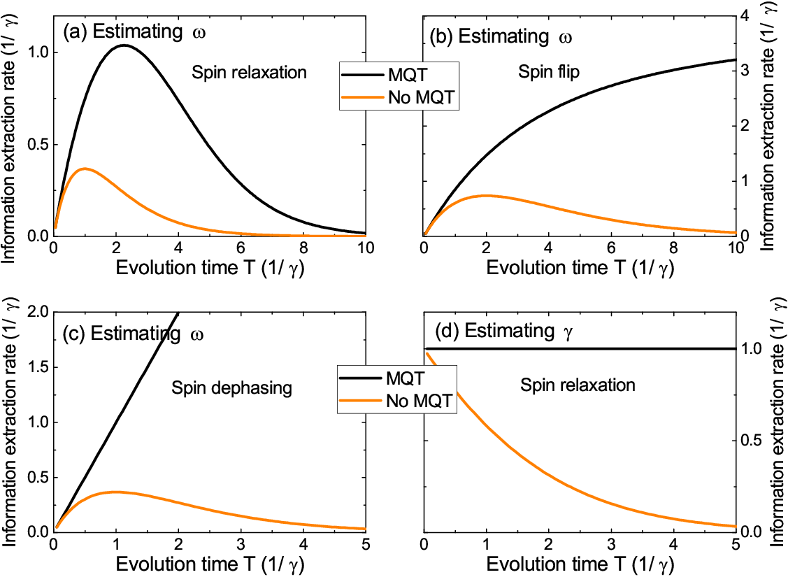
For deterministic parameter estimation, we should take into account the occurrence probabilities of the quantum trajectories. The estimation precision of MQT is determined by
where is the QFI of the conventional approach. For small , the enhancement of relative to could be very large when . In addition, MQT also shortens the total time cost: once a quantum jump is detected, we should immediately stop the current measurement cycle (because the trajectory with a quantum jump has no QFI) and start the next measurement cycle. In this case, the average time cost for each measurement cycle is
| (29) |
which is shorter than , especially when is small. Since the total time cost of repeated measurement cycles is , the estimation precision per unit time, i.e., the sensitivity [cf. Eq. (27)], is determined by the information extraction rate
where the inequality is saturated at . For comparison, the information extracting rate of the conventional method is
where the inequality is saturated at . Therefore, MQT enhances the long-time information extraction rate by a factor although both and exhibit the same exponential decay, as shown in Fig. 3(a).
For the spin flip channel, the jumpless trajectory [Eq. (22)] contains the QFI
that attains the Heisenberg scaling with respect to , while the trajectory with quantum jumps at [Eq. (23)] contains the QFI
where starts from at and reverses its sign at . Physically, every quantum jump reverses the direction of the phase accumulation [manifested as the sign reversal of ] and is the “net” phase accumulation time. For example, we consider the trajectory with a single quantum jump at . Starting from an initial state , the quantum probe first evolves as and then undergoes a spin flip into the state , and then evolve into the final state , so its “net” phase accumulation time is , which coincides with .
Here the Heisenberg scaling of again motivates a probabilistic parameter estimation protocol based on preparing the jumpless trajectory: successful preparations with evolution time and herald the estimation precision , which attains the Heisenberg scaling with respect to . The drawback is that the success probability for each preparation decreases with increasing , so this probabilistic protocol reduces the workload of data processing at the cost of reducing the fundamental estimation precision. For deterministic parameter estimation, we average the QFIs of every trajectory over their occurrence probabilities to obtain
For comparison, the information extraction rate of the conventional method is
Thus MQT avoids the long-time exponential decay of the sensitivity (i.e., precision per unit time), as shown in Fig. 3(b). Physically, the jumpless trajectory has a negligible occurrence probability, so the long-time linear scaling comes from the QFIs of other trajectories: the random quantum jumps leads to random sign reversal of , so and hence the QFI of each trajectory increase linearly with on average, similar to a random walk. MQT gives access to this trajectory-resolved QFI, as opposed to the ensemble QFI from the conventional method.
When we take into account the finite interval between successive syndrome measurements in QEC-based MQT for the spin-flip channel, we obtain
| (30) |
under the condition and , where and is the total number of syndrome measurements during the interval . When the syndrome measurements are much faster than the decoherence (), approaches the ideal results in Table 1. When each syndrome measurement is imperfect, we can combine several adjacent imperfect syndrome measurements into a composite measurement to suppress the measurement error exponentially.
Finally, we turn to the spin dephasing channel. Interestingly, each quantum jump merely flips the phase between and without affecting the phase accumulation [Eq. (25)], so every quantum trajectory contain the same QFI
| (31) |
in contrast to the conventional method:
So MQT can restore the Heisenberg scaling of the estimation precision, as shown in Fig. 3(c). Unfortunately, QEC-based MQT for the dephasing channel of a single spin-1/2 is not possible, so direct measurement over the environment is necessary. For multiple qubits, the key to the recovery of the Heisenberg scaling for estimating is and the preservation of the QFI under the quantum jump [see the discussions after Eq. (18)]. When this condition is satisifed, QEC-based MQT can be used to recover the Heisenberg scaling (see Appendix B for an example).
III.3 Estimation of
For the spin relaxation channel, the estimation precision of MQT is determined by at . By contrast, the estimation precision of the conventional method is determined by at . Thus MQT avoids the exponential loss of the QFI in the conventional method. In addition, it also shortens the total time cost from to [Eq. (29)]. The information extraction rate, which determines the sensitivity , is
| (32) |
where the inequality is saturated at . The information extracting rate of the conventional method is
| (33) |
where the inequality is saturated at . Therefore, MQT avoids the long-time exponential loss of the sensitivity, as shown in Fig. 3(d).
For the spin flip channel, the information about is entirely the CFI in the timings of the quantum jumps: . The information extraction rate from the MQT is
| (34) |
The information extraction rate of the conventional method is
| (35) |
where are the populations of in the initial state and the inequality is saturated at and . Equation (35) is also the ultimate precision bound [102] for adaptive estimation of the dephasing rate without MQT. Comparing Eq. (34) to Eq. (35), we see that MQT avoids the long-time exponential loss of the sensitivity. At , including the finite interval between successive syndrome measurements in QEC-based MQT for the spin-flip channel amounts to a multiplicative factor (with and ) to . When , approaches the ideal results in Table 1. For the spin dephasing channel, we obtain exactly the same results, with () playing the role of (.
IV Conclusion
Quantum enhanced parameter estimation has widespread applications in many fields. An important issue is to protect the estimation precision against the noise-induced decoherence. For this purpose, we have developed a general theoretical framework for improving the precision of parameter estimation by monitoring the noise-induced quantum trajectories (MQT) of the quantum probe and further establish its connection to the purification-based approach to quantum parameter estimation [61]. For Markovian environment, we provide a superoperator approach to determining the fundamental bounds on the estimation precision. This approach may provide exact analytical expressions for some simple models. MQT can be achieved in two ways: (i) Any quantum trajectories can be monitored by directly monitoring the environment, which is experimentally challenging for realistic noises. (ii) Certain quantum trajectories can also be monitored by frequently measuring the quantum probe (without monitoring the environment) via ancilla-assisted encoding and error detection, as used in quantum error correction (QEC). This QEC-based MQT makes certain MQT feasible and further establishes an interesting connection between MQT and the metrology protocols based on full QEC [21, 22, 23, 24, 25, 26, 27, 28]. We apply MQT to the estimation of the level splitting and the decoherence rate of a spin-1/2 under three decoherence channels: spin relaxation, spin flip, and spin dephasing. We find that it can significantly improve the precision for estimating under the spin relaxation channel, avoid the exponential loss of the precision for estimating (estimating ) under all the decoherence channels (under the spin flip channel) and recover the Heisenberg scaling for estimating under the spin dephasing channel.
Acknowledgements.
This work was supported by the MOST of China (Grants No. 2014CB848700), the NSFC (Grants No. 11322542, No. 11704308, No. 11604261, and No. 11547166), and the NSFC program for “Scientific Research Center” (Grant No. U1530401).Appendix A Framework of quantum parameter estimation

Here we provide a self-contained introduction to the typical framework and important concepts in quantum parameter estimation. A typical (non-adaptive) parameter estimation protocol using a quantum probe to estimate an unknown, real parameter consists of three steps (Fig. 4):
- 1.
The quantum probe starts from an initial state and undergoes certain -dependent evolution into a final state that depends on . This step imprints the information about into the final state . The information contained in is quantified by the quantum Fisher information (QFI).
- 2.
The quantum probe undergoes a measurement, which produces an outcome according to certain probability distribution. In this step, the quantum Fisher information contained in is transferred into the classical information in the measurement outcome. The information contained in each outcome is quantified by the classical Fisher information (CFI) , which obeys
(36) - 3.
Steps 1-2 are repeated times and the outcomes are processed to yield an estimator to the unknown parameter . In this step, the total CFI contained in the outcomes is converted to the estimation precision, as quantified by the statistical error of the estimator:
(37) where denotes the average over a lot of estimators obtained by repeating steps 1-3 many times. For unbiased estimators obeying , the precision is fundamentally limited by the inequality
(38)
A.1 Quantum Fisher information
The amount of information about contained in a general -dependent quantum state is quantified by its QFI [80]
where is the so-called symmetric logarithmic derivative operator: it is an Hermitian operator defined through [79]
The QFI is invariant under any -independent unitary transformations. For a pure state , we have and hence
| (39) |
For a general mixed state with the spectral decomposition , its QFI is [103, 104, 105, 106]
where are nonzero eigenvalues of , are the corresponding ortho-normalized eigenstates, and is the QFI of the pure state [see Eq. (39)]. For a two-level system, its density matrix can always be expressed in terms of the Pauli matrices as , where is the Bloch vector. The QFI for such a state is [107, 108, 16]
where the second term is absent when , i.e., when is a pure state. When is the direct product state of quantum probes, its QFI is additive: .
The importance of the QFI for parameter estimation is manifested in the inequalities Eqs. (36) and (38). Namely, given and hence , the precision of any unbiased estimator from repetitions of any measurement is limited by the inequality
| (40) |
known as the quantum Cramér-Rao bound [79, 80]. Saturating this bound requires saturating Eqs. (36) and (38) simultaneously, i.e., using optimal measurements to convert all the QFI into the CFI and using optimal unbiased estimators to convert all the CFI into the precision of the estimator.
A.2 Classical Fisher information and optimal measurements
A general measurement with discrete outcomes is described by the positive-operator valued measure (POVM) elements satisfying the completeness relation . Given a quantum state , it yields an outcome according to the probability distribution that depends on . The amount of information about contained in each outcome is quantified by the CFI [78]:
| (41) |
For continuous outcomes, we need only replace by everywhere. The inequality Eq. (36) expresses the simple fact that no new information about can be generated in the measurement process: those measurements that convert all (part) of the QFI into the CFI are called optimal (non-optimal). Given , the optimal measurement is not unique. The projective measurement on the symmetric logarithmic derivative operator has been identified [80] as an optimal measurement.
A.3 Optimal unbiased estimators
Given the measurement distribution and hence the CFI of each outcome, the precision of any unbiased estimator constructed from the outcomes of repeated measurements is limited by the Cramér-Rao bound Eq. (38), which expresses the simple fact that no new information about can be generated in the data processing: optimal (non-optimal) unbiased estimators convert all (part) of the CFI into the useful information quantified by the precision . In the limit of large , two kinds of estimators are known to be unbiased and optimal: the maximum likelihood estimator and the Bayesian estimator [78], as we introduce now.
Before any measurements, our prior knowledge about the unknown parameter is quantified by certain probability distribution , e.g., a -like distribution corresponds to knowing exactly, a flat distribution corresponds to completely no knowledge about , while a Gaussian distribution corresponds to knowing to be with a typical uncertainty .
Upon getting the first outcome , our knowledge about is immediately refined from to
according to the Bayesian rule [109], where is a normalization factor ensuring is normalized to unity: . Here is the posterior probability distribution of conditioned on the outcome of the measurement being : its parametric dependence on means that different measurement outcomes leads to different refinement of knowledge about .
Upon getting the second outcome , our knowledge is immediately refined from to
where is a normalization factor for the posterior distribution . If we omit the trivial normalization factors, then the measurement-induced knowledge refinement becomes
Upon getting outcomes , our knowledge about is quantified by the posterior distribution
up to a trivial normalization factor, where is the probability for getting the outcome . The posterior distribution completely describe our state of knowledge about . Nevertheless, sometimes a single number, i.e., an unbiased estimator, is required as the best guess to . There are two well-known estimators: the maximum likelihood estimator [78]
| (42) |
is the peak position of as a function of , while the Bayesian estimator [78]
| (43) |
is the average of . For large , both estimators are unbiased and optimal: and , where or , and denotes the average over a large number of estimators obtained by repeating the -outcome estimation scheme many times and is defined as Eq. (37) or
| (44) |
Appendix B Monitoring dephasing of logical qubits
We consider an odd number of spin-1/2’s and each spin-1/2 is subjected to an independent spin dephasing channel. The quantum jump operator of the dephasing channel leads to random transitions between the two eigenstates of during the evolution. We define the -component syndrome operator , where is the Pauli matrix for the th spin-1/2. The code subspace as spanned by [21, 24]
is an eigensubspace of with eigenvalue for every component of . This allows us to monitor the simultaneous quantum jump of at most qubits [21, 24], e.g, the quantum jump of the th spin-1/2 switches the sign of the th and the th component of , while leaves other components of intact. When the Hamiltonian commutes with the syndrome operator, monitoring the quantum jump does not affect the Hamiltonian evolution. When the Hamiltonian further commutes with all the quantum jump operators , the quantum jump does not affect the Hamiltonian evolution. In this case, MQT can fully recover the estimation precision in the noiseless case.
As an example, we consider , where maps to and to . This Hamiltonian commutes with the syndrome operator and all the quantum jump operators. The initial state lies inside the code subspace. In the absence of quantum jumps, the final state is , whose QFI attains the Heisenberg scaling with respect to the time cost . By frequently measuring the syndrome operator, we can track the simultaneous phase flip of at most qubits. Since the phase flip commute with , they always map () to another eigenstate of with the same eigenvalue, thus all the detectable quantum jumps do not cause the loss of the QFI. For example, a quantum jump of the th qubit at time maps the -qubit state to , where () is still an eigenstate of with the same eigenvalue (). Afterwards, the evolution under leads to the final state , which contains the same QFI as the jumpless state. Therefore, MQT allows us to continuously track the quantum trajectory and hence recover the Heisenberg scaling of the estimation precision without error correction, as long as in between two round of syndrome measurements, the number of phase-flipped qubits do not exceed . By contrast, when the quantum trajectories are not monitored, the QFI of the non-selective final state would decay to zero on time scales single-qubit decoherence time.
The results above are consistent with the conclusion of Refs. [69, 68] since the Hamiltonian lies outside the Lindblad span of all the decoherence channels. The results above can also be generalized to logical qubits, where each logical qubit is composed of qubits through the -qubit phase-flip code and is driven by the Hamiltonian . Starting from the initial state , all the detectable quantum trajectories contain the same QFI , which gives the Heisenberg scaling for the estimation precision about .
Appendix C Estimation precision for spin-flip channel
C.1 Ideal continuous monitoring
For ideal, continuous monitoring of the quantum jump (i.e., spin flip), the normalized quantum trajectory with quantum jumps at has a QFI
with occurence probability density . For , they reduce to the QFI and the occurence probability of the jumpless trajectory. The trajectory-averaged QFI follows by straightforward calculation:
The sum is equal to with , so we obtain the listed in Table I. Since is independent of and the timings of the quantum jumps, Eq. (18) gives and
| (45) |
where
is the probability for quantum jumps during .
C.2 Realistic QEC-based monitoring
When we use QEC-based MQT with the syndrome operator with eigenvalues (see Sec. II.5), the interval between successive syndrome measurements is finite. The total evolution interval is divided into segments of length sandwiched by syndrome measurements at . At , the initial state of the spin-1/2 and the ancilla is an eigenstate of the syndrome operator with eigenvalue . For clarity we use ( or ) to denote the outcome of the th syndrome measurement, where . If the th syndrome measurement reports a sign switch, i.e., , then the spin-1/2 undergoes an odd number of quantum jumps during , otherwise (i.e., ) the spin-1/2 undergoes an even number of quantum jumps during . If , then the possibility of multiple quantum jumps between neighboring syndrome measurement is exponentially small, so the syndrome measurements can well resolve individual quantum jumps. Otherwise, the syndrome measurements only give little information about the quantum jumps.
First, we derive the evolution of the quantum trajectories between the th and the th syndrome measurements. Suppose the previous syndrome measurements give the outcomes and the un-normalized quantum trajectory immediately after the th syndrome measurement is
which is an eigenstate of with eigenvalue . The non-selective evolution during gives the non-selective final state:
where and are superoperators:
, , , and Since each quantum jump leads to the exchanges and hence and , we identify () as the un-normalized quantum trajectory containing an even (odd) number of quantum jumps during . In other words, the un-normalized quantum trajectory at is if the th syndrome measurement reports a sign switch, or otherwise. Their occurence probabilities are , so the non-selective evolution is trace-preserving:. When , the occurence probabilities of are and , respectively.
This single-step evolution can be iterated times to yield the quantum trajectories at . Specifically, if only the syndrome measurements at report sign switches, then the un-normalized quantum trajectory at is
and its occurence probability
is independent of . Since is independent of , the CFI about vanishes: , and the CFI about follows from Eq. (18) as
where is the probability for quantum jumps during and is the binomial coefficient. Next, we calculate the QFIs in the normalized quantum trajectories: .
When , we have , , and hence and , so (for even ) or (for odd ) is independent of and hence give zero trajectory QFI about . In this case, the total information from MQT is .
When , to obtain explicit analytical expression, we assume and , so that , , and hence
where
The trajectory-QFI is
Averaging the trajectory-QFI over their occurence probabilities gives
where is the largest integer not greater than and we have used and . Performing the summation gives Eq. (30) of the main text.
References
- [1] V. Giovannetti, S. Lloyd, and L. Maccone, Phys. Rev. Lett. 96, 010401 (2006).
- [2] C. L. Degen, F. Reinhard, and P. Cappellaro, Rev. Mod. Phys. 89, 035002 (2017).
- [3] C. M. Caves, Phys. Rev. D 23, 1693 (1981).
- [4] L. S. Collaboration, Nat. Photon. 7, 613 (2013).
- [5] D. J. Wineland, J. J. Bollinger, W. M. Itano, F. L. Moore, and D. J. Heinzen, Phys. Rev. A 46, R6797 (1992).
- [6] J. J. . Bollinger, W. M. Itano, D. J. Wineland, and D. J. Heinzen, Phys. Rev. A 54, R4649 (1996).
- [7] D. Budker and M. Romalis, Nat. Phys. 3, 227 (2007).
- [8] L. Rondin, J.-P. Tetienne, T. Hingant, J.-F. Roch, P. Maletinsky, and V. Jacques, Rep. Prog. Phys. 77, 056503 (2014).
- [9] J. P. Dowling, Contemp. Phys. 49, 125 (2008).
- [10] J. Borregaard and A. S. Sørensen, Phys. Rev. Lett. 111, 090801 (2013).
- [11] W. Yang, W.-L. Ma, and R.-B. Liu, Rep. Prog. Phys. 80, 016001 (2017).
- [12] J. R. Maze, P. L. Stanwix, J. S. Hodges, S. Hong, J. M. Taylor, P. Cappellaro, L. Jiang, M. V. G. Dutt, E. Togan, A. S. Zibrov, A. Yacoby, R. L. Walsworth, and M. D. Lukin, Nature 455, 644 (2008).
- [13] J. M. Taylor, P. Cappellaro, L. Childress, L. Jiang, D. Budker, P. R. Hemmer, A. Yacoby, R. Walsworth, and M. D. Lukin, Nat. Phys. 4, 810 (2008).
- [14] N. Zhao, J.-L. Hu, S.-W. Ho, J. T. K. Wan, and R.-B. Liu, Nat. Nanotechnol. 6, 242 (2011).
- [15] J. Cai, F. Jelezko, M. B. Plenio, and A. Retzker, New J. Phys. 15, 013020 (2013).
- [16] Y.-L. Li, X. Xiao, and Y. Yao, Phys. Rev. A 91, 052105 (2015).
- [17] W. Yang, Z.-Y. Wang, and R.-B. Liu, Front. Phys. 6, 2 (2011).
- [18] Y. Matsuzaki, S. C. Benjamin, and J. Fitzsimons, Phys. Rev. A 84, 012103 (2011).
- [19] A. W. Chin, S. F. Huelga, and M. B. Plenio, Phys. Rev. Lett. 109, 233601 (2012).
- [20] R. Chaves, J. B. Brask, M. Markiewicz, J. Kolodynski, and A. Acin, Phys. Rev. Lett. 111, 120401 (2013).
- [21] W. Dür, M. Skotiniotis, F. Fröwis, and B. Kraus, Phys. Rev. Lett. 112, 080801 (2014).
- [22] E. M. Kessler, I. Lovchinsky, A. O. Sushkov, and M. D. Lukin, Phys. Rev. Lett. 112, 150802 (2014).
- [23] G. Arrad, Y. Vinkler, D. Aharonov, and A. Retzker, Phys. Rev. Lett. 112, 150801 (2014).
- [24] X.-M. Lu, S. Yu, and C. H. Oh, Nat. Commun. 6, 7282 (2015).
- [25] D. A. Herrera-Martí, T. Gefen, D. Aharonov, N. Katz, and A. Retzker, Phys. Rev. Lett. 115, 200501 (2015).
- [26] T. Unden, P. Balasubramanian, D. Louzon, Y. Vinkler, M. B. Plenio, M. Markham, D. Twitchen, A. Stacey, I. Lovchinsky, A. O. Sushkov, M. D. Lukin, A. Retzker, B. Naydenov, L. P. McGuinness, and F. Jelezko, Phys. Rev. Lett. 116, 230502 (2016).
- [27] M. Bergmann and P. van Loock, Phys. Rev. A 94, 012311 (2016).
- [28] Y. Matsuzaki and S. Benjamin, Phys. Rev. A 95, 032303 (2017).
- [29] Q. Zheng, L. Ge, Y. Yao, and Q.-j. Zhi, Phys. Rev. A 91, 033805 (2015).
- [30] M. Hirose and P. Cappellaro, Nature 532, 77 (2016).
- [31] J. Liu and H. Yuan, Phys. Rev. A 96, 012117 (2017).
- [32] Y. Watanabe, T. Sagawa, and M. Ueda, Phys. Rev. Lett. 104, 020401 (2010).
- [33] A. Laraoui, F. Dolde, C. Burk, F. Reinhard, J. Wrachtrup, and C. A. Meriles, Nat. Commun. 4, 1651 (2013).
- [34] Q.-S. Tan, Y. Huang, X. Yin, L.-M. Kuang, and X. Wang, Phys. Rev. A 87, 032102 (2013).
- [35] N. Zhao, J. Wrachtrup, and R.-B. Liu, Phys. Rev. A 90, 032319 (2014).
- [36] N. Zhao and Z. Q. Yin, Phys. Rev. A 90, 042118 (2014).
- [37] J. M. Boss, K. Chang, J. Armijo, K. Cujia, T. Rosskopf, J. R. Maze, and C. L. Degen, Phys. Rev. Lett. 116, 197601 (2016).
- [38] W.-L. Ma and R.-B. Liu, Phys. Rev. Applied 6, 054012 (2016a).
- [39] W.-L. Ma and R.-B. Liu, Phys. Rev. Applied 6, 024019 (2016b).
- [40] F. Yan, S. Gustavsson, J. Bylander, X. Jin, F. Yoshihara, D. G. Cory, Y. Nakamura, T. P. Orlando, and W. D. Oliver, Nat. Commun. 4, 2337 (2013).
- [41] M. Loretz, T. Rosskopf, and C. L. Degen, Phys. Rev. Lett. 110, 017602 (2013).
- [42] J. E. Lang, R. B. Liu, and T. S. Monteiro, Phys. Rev. X 5, 041016 (2015).
- [43] S. Kotler, N. Akerman, Y. Glickman, A. Keselman, and R. Ozeri, Nature 473, 61 (2011).
- [44] G. de Lange, D. Ristè, V. V. Dobrovitski, and R. Hanson, Phys. Rev. Lett. 106, 080802 (2011).
- [45] G. de Lange, Z. H. Wang, D. Riste, V. V. Dobrovitski, and R. Hanson, Science 330, 60 (2010).
- [46] G. A. Álvarez and D. Suter, Phys. Rev. Lett. 107, 230501 (2011).
- [47] J. Medford, L. Cywiński, C. Barthel, C. M. Marcus, M. P. Hanson, and A. C. Gossard, Phys. Rev. Lett. 108, 086802 (2012).
- [48] N. Bar-Gill, L. Pham, C. Belthangady, D. Le Sage, P. Cappellaro, J. Maze, M. Lukin, A. Yacoby, and R. Walsworth, Nat. Commun. 3, 858 (2012).
- [49] J. T. Muhonen, J. P. Dehollain, A. Laucht, F. E. Hudson, R. Kalra, T. Sekiguchi, K. M. Itoh, D. N. Jamieson, J. C. McCallum, A. S. Dzurak, and A. Morello, Nat Nano 9, 986 (2014).
- [50] N. Zhao, J. Honert, B. Schmid, M. Klas, J. Isoya, M. Markham, D. Twitchen, F. Jelezko, R.-B. Liu, H. Fedder, and J. Wrachtrup, Nat Nano 7, 657 (2012).
- [51] S. Kolkowitz, Q. P. Unterreithmeier, S. D. Bennett, and M. D. Lukin, Phys. Rev. Lett. 109, 137601 (2012).
- [52] T. H. Taminiau, J. J. T. Wagenaar, T. van der Sar, F. Jelezko, V. V. Dobrovitski, and R. Hanson, Phys. Rev. Lett. 109, 137602 (2012).
- [53] P. London, J. Scheuer, J.-M. Cai, I. Schwarz, A. Retzker, M. B. Plenio, M. Katagiri, T. Teraji, S. Koizumi, J. Isoya, R. Fischer, L. P. McGuinness, B. Naydenov, and F. Jelezko, Phys. Rev. Lett. 111, 067601 (2013).
- [54] T. Staudacher, F. Shi, S. Pezzagna, J. Meijer, J. Du, C. a. Meriles, F. Reinhard, and J. Wrachtrup, Science 339, 561 (2013).
- [55] H. J. Mamin, M. Kim, M. H. Sherwood, C. T. Rettner, K. Ohno, D. D. Awschalom, and D. Rugar, Science 339, 557 (2013).
- [56] F. Shi, X. Kong, P. Wang, F. Kong, N. Zhao, R.-B. Liu, and J. Du, Nat. Phys. 10, 21 (2014).
- [57] X.-M. Lu, X. Wang, and C. P. Sun, Phys. Rev. A 82, 042103 (2010).
- [58] K. Berrada, Phys. Rev. A 88, 035806 (2013).
- [59] P. Sekatski, M. Skotiniotis, and W. Dür, New Journal of Physics 18, 073034 (2016).
- [60] Y.-S. Wang, C. Chen, and J.-H. An, New J. Phys. 19, 113019 (2017).
- [61] A. Fujiwara and H. Imai, Journal of Physics A: Mathematical and Theoretical 41, 255304 (2008).
- [62] B. M. Escher, R. L. de Matos Filho, and L. Davidovich, Nat. Phys. 7, 406 (2011).
- [63] R. Demkowicz-Dobrzanski, J. Kolodynski, and M. Guta, Nat. Commun. 3, 1063 (2012).
- [64] B. M. Escher, L. Davidovich, N. Zagury, and R. L. de Matos Filho, Phys. Rev. Lett. 109, 190404 (2012).
- [65] M. Jarzyna and R. Demkowicz-Dobrzański, Phys. Rev. Lett. 110, 240405 (2013).
- [66] R. Demkowicz-Dobrzański and L. Maccone, Phys. Rev. Lett. 113, 250801 (2014).
- [67] R. Demkowicz-Dobrzański, M. Jarzyna, and J. Kołodyński, Chapter Four - Quantum Limits in Optical Interferometry, edited by E. Wolf, Progress in Optics, Vol. 60 (Elsevier, 2015) pp. 345 – 435.
- [68] R. Demkowicz-Dobrzański, J. Czajkowski, and P. Sekatski, Phys. Rev. X 7, 041009 (2017).
- [69] S. Zhou, M. Zhang, J. Preskill, and L. Jiang, Nature Communications 9, 78 (2018).
- [70] C. Catana and M. u. u. u. u. Guţă, Phys. Rev. A 90, 012330 (2014).
- [71] F. Albarelli, M. A. C. Rossi, M. G. A. Paris, and M. G. Genoni, New J. Phys. 19, 123011 (2017).
- [72] F. Albarelli, M. A. C. Rossi, D. Tamascelli, and M. G. Genoni, Quantum 2, 110 (2018).
- [73] S. Gammelmark and K. Mølmer, Phys. Rev. A 87, 032115 (2013).
- [74] S. Gammelmark and K. Mølmer, Phys. Rev. Lett. 112, 170401 (2014).
- [75] M. G. Genoni, Phys. Rev. A 95, 012116 (2017).
- [76] H. Yuan and C.-H. F. Fung, Phys. Rev. A 96, 012310 (2017).
- [77] P. Sekatski, M. Skotiniotis, J. Kolodynski, and W. Dur, Quantum 1, 27 (2017).
- [78] S. M. Kay, Fundamentals of Statistical Signal Processing: Estimation Theory (Prentice-Hall, 1993).
- [79] C. W. Helstrom, Quantum Detection and Estimation Theory (Academic press, New York, 1976).
- [80] S. L. Braunstein and C. M. Caves, Phys. Rev. Lett. 72, 3439 (1994).
- [81] C. M. Kropf, C. Gneiting, and A. Buchleitner, Phys. Rev. X 6, 031023 (2016).
- [82] A. Smirne, J. Kołodyński, S. F. Huelga, and R. Demkowicz-Dobrzański, Phys. Rev. Lett. 116, 120801 (2016).
- [83] J. Combes, C. Ferrie, Z. Jiang, and C. M. Caves, Phys. Rev. A 89, 052117 (2014).
- [84] C. Ferrie, Phys. Rev. A 90, 014101 (2014).
- [85] S. Alipour and A. T. Rezakhani, Phys. Rev. A 91, 042104 (2015).
- [86] S. Ng, S. Z. Ang, T. A. Wheatley, H. Yonezawa, A. Furusawa, E. H. Huntington, and M. Tsang, Phys. Rev. A 93, 042121 (2016).
- [87] J. Kolodynski and R. Demkowicz-Dobrzanski, New J. Phys. 15, 073043 (2013).
- [88] M. B. Plenio and P. L. Knight, Rev. Mod. Phys. 70, 101 (1998).
- [89] S. Gleyzes, S. Kuhr, C. Guerlin, J. Bernu, S. Deléglise, U. Busk Hoff, M. Brune, J.-M. Raimond, and S. Haroche, Nature 446, 297 (2007).
- [90] J. Piilo, S. Maniscalco, K. Härkönen, and K.-A. Suominen, Phys. Rev. Lett. 100, 180402 (2008).
- [91] Y. Yu, S.-L. Zhu, G. Sun, X. Wen, N. Dong, J. Chen, P. Wu, and S. Han, Phys. Rev. Lett. 101, 157001 (2008).
- [92] A. N. Vamivakas, C.-Y. Lu, C. Matthiesen, Y. Zhao, S. Falt, A. Badolato, and M. Atature, Nature 467, 297 (2010).
- [93] A. Delteil, W. B. Gao, P. Fallahi, J. Miguel-Sanchez, and A. Imamoglu, Phys. Rev. Lett. 112, 116802 (2014).
- [94] P. Campagne-Ibarcq, P. Six, L. Bretheau, A. Sarlette, M. Mirrahimi, P. Rouchon, and B. Huard, Phys. Rev. X 6, 011002 (2016).
- [95] M. Naghiloo, N. Foroozani, D. Tan, A. Jadbabaie, and K. W. Murch, Nat. Commun. 7, 11527 (2016).
- [96] A. G. Kofman, S. Ashhab, and F. Nori, Physics Reports 520, 43 (2012).
- [97] J. Dressel, M. Malik, F. M. Miatto, A. N. Jordan, and R. W. Boyd, Rev. Mod. Phys. 86, 307 (2014).
- [98] A. N. Jordan, J. Martínez-Rincón, and J. C. Howell, Phys. Rev. X 4, 011031 (2014).
- [99] C. Ferrie and J. Combes, Phys. Rev. Lett. 112, 040406 (2014).
- [100] R. Schirhagl, K. Chang, M. Loretz, and C. L. Degen, Annual Review of Physical Chemistry, Annu. Rev. Phys. Chem. 65, 83 (2014).
- [101] M. A. Nielsen and I. L. Chuang, Quantum Computation and Quantum Information (Cambridge University, Cambridge, England, 2000).
- [102] S. Pirandola and C. Lupo, Phys. Rev. Lett. 118, 100502 (2017).
- [103] S. Knysh, V. N. Smelyanskiy, and G. A. Durkin, Phys. Rev. A 83, 021804 (2011).
- [104] Y. M. Zhang, X. W. Li, W. Yang, and G. R. Jin, Phys. Rev. A 88, 043832 (2013).
- [105] J. Liu, X. Jing, and X. Wang, Phys. Rev. A 88, 042316 (2013).
- [106] X.-X. Jing, J. Liu, W. Zhong, and X.-G. Wang, Communications in Theoretical Physics 61, 115 (2014).
- [107] J. Dittmann, J. Phys. A: Math. Gen. 32, 2663 (1999).
- [108] W. Zhong, Z. Sun, J. Ma, X. Wang, and F. Nori, Phys. Rev. A 87, 022337 (2013).
- [109] U. von Toussaint, Rev. Mod. Phys. 83, 943 (2011).