Neutrino masses and gauged lepton number
Abstract
We investigate the tree-level neutrino mass generation in the gauged lepton model recently proposed by us [1]. With the addition of one Standard Model(SM) singlet, , and one SM triplet scalar, , realistic lepton masses can be accommodated. The resulting magnitude of neutrino mass is given by , where and are the vacuum expectation values of and , respectively, and it is automatically of the inverse see-saw type. Since is the lepton number violation scale we take it to be high, i.e. . Moreover, the induced lepton flavor violating processes and the phenomenology of the peculiar triplet are studied. An interesting bound, GeV, is obtained when taking into account the neutrino mass generation, , and the limits from oblique parameters, and . Collider phenomenology of the SM triplets is also discussed.
1 Introduction
It is now generally accepted that neutrino oscillation data indicate that at least two of the three active neutrinos have nonvanishing masses. This cannot be accommodated in the minimal Standard Model (SM)without adding new degrees of freedom such as two or more SM right-handed neutrinos. However, neutrino masses can be generated by the addition of the Weinberg operator [2], . This nonrenormalizable dimension five operator takes the form of , where is the SM Higgs field, denotes a SM lefthanded lepton doublet, is a free dimensionless parameter, and is an unknown high scale. After takes on a vacuum expectation value GeV, the electroweak symmetry is spontaneously broken, and we get a neutrino mass . Since data indicate that eV, depending on the value of , the scale can range from 1 to TeV. This elegant way of generating neutrino masses using only SM fields comes with the price of nonrenomalizability. Furthermore, it reinforces the idea that the SM is an effective theory and the neutrino masses call for its extension.
Neutrino mass generated from the Weinberg operator is of the Majorana type, and it has lepton number provided the conventional lepton number assignments that all SM charged leptons and their associated neutrinos have and all other SM fields carry are assumed. Also the anti-leptons have . This is a natural consequence if lepton number is a symmetry. Thus, the SM is largely invariant under this symmetry with a very small breaking by the Weinberg operator. However, the nature of this symmetry is unknown. Usually, the total lepton number is taken to be a global symmetry that is broken at a very high scale GeV by two or more SM singlet righthanded neutrinos with Majorana masses of . Integrating them out gives rise to the Weinberg operator, and this is the celebrated type I seesaw mechanism [3, 4, 5, 6, 7]. Doing so raises the question of the origin of the Majorana mass bestowed to . One can add a Majorana mass for by hand. However, our current understanding is that masses of fermions are generated by the Higgs mechanism. It is interesting to also to apply this to . Doing so will lead to the existence of a Goldstone boson in the physical spectrum which can act as a candidate for dark radiation [8, 9].
Moreover, it is phenomenologically and theoretically interesting to investigate the possibility of a gauged and study the spontaneously broken gauge theory. There are several possibilities. One can gauge the total lepton number as in [10]11 1 For other constructions in conjunction with gauged baryon number see[11, 12, 13, 14, 15].. One can also gauge a combination of lepton generation number such as [16, 17]. In Ref.([1]), hereafter referred to as (I), we gauged each lepton family with the usual lepton number assignments for them. Of the just mentioned three examples only the second one is anomaly-free with only the SM fields. Gauging the total lepton will require extra leptons with very exotic lepton charges such as to cancel the anomalies from . In (I), the extra anomalies cancelations require two extra pairs of vector-like doublet leptons with eigenvalues for each family. We also did not include any singlet field, and the Weinberg operator is generated radiatively at 1-loop. The principal source of lepton number violation comes from a SM singlet scalar with which picks up a vacuum expectation value.
In this paper, we study a different mechanism of neutrino mass generation in the gauged lepton number scheme introduced in (I). The extra leptons presented before is sufficient to generate neutrino masses with the aid of a SM triplet scalar and a SM singlet scalar . has whereas is given , with both fields being Higgssed. This naturally leads to an inverse seesaw mechanism (ISM)[18, 19, 20] for active neutrino mass. The novel feature here is that we do not add by hand any SM singlet leptons to implement ISM as is commonly done. The required leptons are dictated by anomaly cancelations. Details will be given in Sec. 3. Since the physics involved with the gauge new gauge boson and the extra leptons are the same as in (I), we will not repeat their phenomenology here. Instead, we focus on neutrino physics and the phenomenology of . We find that has interesting different signatures at high energy colliders from previous studies of Higgs triplets[21, 22, 23, 24, 25], which are commonly employed in the type-II see-saw model[26, 27, 28, 29, 30, 31]. For a recent review see [32].
We organize the paper as follows. The next section we present our anomalies solution for completeness. Then we discuss lepton mass generation for one generation to illustrate the physics. This is followed by a realistic 3-generation study. Sec. 4 gives fits to the neutrino oscillation data. Constraints from charged lepton flavor changing neutral currents are given in Sec.5. Important electroweak precision constraints are studied in Sec. 6. The productions of different new triplet scalars at the LHC and CLIC are examined in Sec. 7. Our conclusions are given in Sec. 8.
2 anomalies cancelations and new fields
We extend the SM gauged group by adding a and is explicitly given as . All SM leptons have the conventional value of . We will concentrate on one family. This can be trivially extended for all 3 SM families.
The new anomaly coefficients are
| (1a) | |||||
| (1b) | |||||
| (1c) | |||||
| (1d) | |||||
| (1e) | |||||
where stands for the lepton-graviton anomaly. While new chiral leptons are introduced to cancel Eq.(1), one also needs to make sure that the SM anomalies of , , and are canceled. It is easy to check that the new leptons in Table.1 cancel the above anomalies.
| Field | |||
|---|---|---|---|
| 2 | |||
| 1 | |||
| 2 | |||
| 1 | |||
| 2 | |||
| 1 |
Since the pair of new leptons are vectorlike, the SM anomalies , , and cancelations are not affected.
The minimal set of scalar fields, by utilizing the triplet scalar for neutrino mass generation, can be obtained by examining the gauge invariant set of lepton bilinears that can be formed from the above fields. They are given in Table.2.
| Field | |||
|---|---|---|---|
| 2 | |||
| 3 | |||
| 1 |
where all , and develop non-zero VEVs.
The Yukawa interactions are
| (2) | |||||
where all the generation indices are suppressed. The full gauge invariant and renormalizable scalar potential reads,
| (3) | |||||
where we have used the bi-doublet form for as below22 2 If a doublet, , transforms under as , then .
| (4) |
The following conditions must hold ()
| (5) |
so as to ensure that the potential is bounded from below.
After SSB,
| (6) |
and the fields can be expanded around their VEVs as
| (7) |
And the minimal condition for the scalar potential become
| (8) | |||
| (9) | |||
| (10) |
Note that do not come into play here. From the above equations, the tree-level mass squared for and are
| (11) |
From phenomenology we expect that (see Sec.8) and before scalar mixings considerations we have
| (12) |
which are above a TeV if takes a phenomenologically interesting value around the electroweak scale. However, in general, is a free parameter.
The scalar potential after SSB gives a small mass splitting between and . The mass squared difference can be worked out to be
| (13) |
which is provided is not much smaller than . Therefore, it is a good approximation to assume that and are degenerate. However, we should keep in mind the mass splitting could be about the Fermi scale.
Similarly, ignoring the contribution from , we have
| (14) | |||
| (15) |
Since we expect that , i.e. lepton symmetry breaking to be above the Fermi scale, we obtain
| (16) |
Thus, it is also required to have . As expected, there will be mixing among the three neutral scalars . They are related to the physical states via the usual unitary rotation given by
| (17) |
Details of this transformation are not important for this study and we will not present them.
For completeness, we discuss the imaginary parts of the scalar fields. is the would-be Goldstone for the gauge boson . Moreover, the would-be Goldstone bosons eaten by , the physical singly charged scalars, , and the pseudoscalar, , can be identified as:
| (18) |
Since from the electroweak precision studies (see Sec. 8), it is a good approximation to treat and as the physical states. Being the only degree of freedom with two units of electric charge, are the physical scalars.
Since the symmetry forbids from coupling to two SM fermions simultaneously, its gauge interactions become the most relevant for phenomenology. From the -covariant derivative we obtain the Feynman rules for its triple couplings to gauge bosons, displayed in Table 3, where stands for the photon, and all the momenta are incoming.
| : | : | ||||
| : | : | ||||
| : | : | ||||
| : | : | ||||
| : | : |
3 Lepton masses for 1 generation
The physics of how the new leptons affect the SM charged leptons is best seen in the one family scenario. In the basis , the Dirac mass matrix is
| (19) |
where . In general the electron will mix with and the mixing depends on and . In that case, the charged-current interaction of the SM leptons could deviate from the canonical SM form due to their mixings with and . Moreover, the SM gauge couplings are flavor non-diagonal. Physically, this mixing must be very small and we can take the limiting case of and eliminate the mixing of the electron with the new charged leptons33 3 Theoretically, these two Yukawa couplings can not be forbidden by any or charge assignment in this model. However, one can obtain the desired Yukawa hierarchy in the split-fermion model if the 5D wave-functions centers are in the order of , where “,” and “;” mean large and small separations in between two adjacent wave functions, respectively, along the fifth dimension, see [33, 34, 35] for some other examples of achieving the hierarchical 4D Yukawa. . In general, we can write the physical mass eigenstates where as
| (20) |
where is the left-handed/right-handed unitary matrix that diagonalizes the charged lepton mass matrix so that . For the limiting case of and with , the mass eigenvalues can be worked out to be
| (21) |
One can see that the leading mass splitting between and , apart from the phase convention, comes from the SM Higgs Yukawa interaction, , and to a very good approximation,
| (22) |
In the basis , the neutrino mass matrix is
| (23) |
and . Again, we consider the case that and . The eigenvalues can be worked out to be around , , and in units of . It is natural to identify the first term as the mass of the active neutrino. For GeV and TeV, the resulting active neutrino mass is about eV. From electroweak precision measurements we expect GeV. We see that the desired neutrino mass can be obtained without much tuning of the Yukawa couplings.
4 3-generation lepton masses
One can extend the above to the realistic 3-generation case. Without losing any generality, we can start with the basis that the Yukawa couplings for are diagonal. And we can go to the basis where the SM charged leptons are in their mass eigenstates by bi-unitary transformation among the and . Similarly, we have the freedom to start with diagonal and sub-matrices.
4.1 Charged lepton mass matrix
For simplicity, let’s consider that , , and the heavy charged lepton are roughly degenerate. Then, in the basis where each entry is a 3-vector in family space, the most general mass matrix for charged leptons looks like
| (24) |
where and are diagonal matrices and is the unit matrix. For convenience, which encodes the small splitting of the heavy charged leptons are separated out from the leading term. One can first perform a rotation among the heavy charged leptons by , which is a generalization of Eq.(22). Then the small perturbation can be separated from the leading order mass eigenvalues,
One can further diagonalize the diagonal block, , by a bi-unitary transformation such that . Or by using
| (33) |
so that
It is clear that the 6 heavy charged leptons will form 3 nearly degenerate pairs. And as in the 1-generation case, the mass splitting for each pair is mainly controlled by . Moreover, they decouple from the SM charged leptons.
4.2 Neutral lepton mass matrix
Using the notation of the charged leptons and factor out the common mass, we write the general neutrino mass matrix as
| (38) |
where is a symmetric matrix with elements , is a general matrix with elements , and now is a diagonal matrix , , to accommodate the small non-degeneracy among the three heavy s. First, the leading mass diagonalization can be made by the same rotation , similar to Eq.(22), as in the charged lepton case. This results in a symmetric matrix, , in the diagonal blocks as the perturbation. Assume there exists an orthogonal transformation , such that , and . Then by using , the re-scaled neutrino mass matrix can be brought into the following form
where , , and . One can see that after this rotation, the leading mass eigenstates are nothing but the Cartesian basis. By the standard perturbation techniques, it is easy to see that the SM neutrinos will acquire nonzero masses at the second order perturbation. For example, at this order,
| (46) |
and it is indeed of the order of as in the 1-generation case.
The active neutrino masses can also be understood diagrammatically. By integrating out the heavy , the corresponding Feynman diagram in the weak basis, displayed in Fig.1, and can be seen to give the same conclusion. It also reveals that the low energy effective operator for active neutrino mass is not given by the Weinberg operator. If we assume a hierarchy that , and is the only beyond SM degree of freedom left below , the active neutrino masses are generated by a dimension six operator where is a constant and is the lepton number breaking scale related to . After picks up a VEV, , the neutrino mass is given by . It is also clear that has a higher dimension than the Weinberg operator. Together with the fact that ., they allow the lepton breaking scale to be much lower than the usual type I seesaw mechanism.

Now, the upper-left sub-matrix, denoted as , of for active neutrinos is in general non-unitary, . This non-unitarity will result in various observable effects. However, one expects that the off-diagonal elements of are of the order of , which is roughly below the current experimental limits, [36, 37]. Therefore, we will leave the comprehensive study of these precision tests to future work.
5 Neutrino oscillations and data fitting
First, we provide a simple, realistic solution which can accommodate the neutrino data. Then we move on to the more general numerical survey where the solutions will be fed into the later study of lepton flavor changing processes.
To simplify the discussion, we assume that the heavy ’s are degenerate(), , and all the Yukawa couplings in are of the same order and there is no hierarchy among them. The mass matrix looks like
| (47) |
where is an unknown overall constant which controls the amplitude of perturbation and the elements of are of . As discussed previously, in the leading approximation, the active neutrino mass matrix reads
| (48) |
If is highly democratic, namely,
| (49) |
the resulting active neutrino mass matrix also has the pattern which is of rank one and it has two zero eigenvalues. It naturally leads to the normal hierarchical neutrino masses. Taking into account the data, the realistic mass matrix for normal hierarchy(NH) instead takes the form
| (50) |
if , and, to simplify the discussion we set . A simple solution to arrive such pattern is
| (51) |
which has the apparent symmetry. This can be realized in the extra-dimensional models by arranging the amount of overlap in higher dimensional fermion wavefunctions, see for example [34, 35, 33].
On the other hand, a more subtle construction of is required to accommodate the inverted hierarchy( IH ) case. For example, if , the following realistic neutrino masses matrix
| (52) |
can be generated by
| (53) |
For both NH and IH cases, . Taking GeV and TeV, we have . This simple solution with gives us a rough idea of the Yukawa coupling strengths.
For the realistic data fitting, we perform a comprehensive numerical scan with the working assumption that and that the heavy ’s are nearly degenerate. These assumption can be relaxed giving rise to more free parameters to fit the data. Moreover, the Yukawa couplings are taken to be complex in the numerical study to accommodate the nonzero CP phase, which current data give a hint of. However, it is clear that the resulting neutrino mass is about . We adopt the following ranges from [38] for the neutrino oscillation parameters. For NH,
| (54) |
As for the IH case, the corresponding ranges are:
| (55) |
The lightest neutrino masses, , for both NH and IH are allowed to vary in the range between eV and eV so that the cosmological bound, eV at C.L.(from CMB spectrum and gravitational lensing data only)[39]44 4 This upper limit has been improved to eV ( or eV ) at C.L.[40] recently. , can be met. Once is fixed, can be determined from the measured mass squared differences. Then the effective active neutrino mass matrix can be obtained by
| (56) |
In the standard parametrization, the rotation matrix is given by55 5 In general where is the unitary matrix that diagonalizes the SM charged leptons mass matrix and is the neutrino rotation matrix. In the limit that the decouples from the we can take .
| (57) |
where the shorthand and the like are used. Each element of the Yukawa matrix is a random number in between and times an overall unknown factor with either sign. And we require that the ratio of the largest to the smallest absolute values in to be smaller than . About such solutions are prepared for both NH and IH cases. The realistic Yukawa coupling configurations can be used for predicting the lepton flavor violating processes. The results will be displayed in the next section.
6 , and
With this rich exotic leptons introduced for anomaly cancelations it is important to examine the constraints from charged lepton flavor violation (CLFV) searches. The process can be mediated by triplet running in the loop, see Fig.2.

In the lepton mass basis, with the rotation, the triplet coupling can be approximated as
| (58) | |||||
where are the generation indices, and denote the different mass eigenstates within each generation.
The 1-loop contributions can be calculated to be
| (59) |
where , , and
| (60) |
See Fig.3 for the plot of this function.
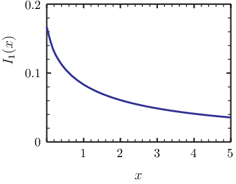
When and , the loop function can be expanded as
| (61) | |||||
| (62) |
The first term in the square bracket of Eq.(59) is the contribution where the photon attaches to the heavy charged lepton. The second and third terms are the contributions where the photon attaches to the and , respectively. Because of the electric charge, the contribution has an extra factor 2. Note also the one half factor associated with the contribution which is due to the extra factor in the singly charged triplet-fermion vertex coupling. Moreover, assuming that ( so that all ) the can be related to the neutrino mass and eliminating the dependence,
| (63) |
which is negligibly small.
Similar calculation can be carried out for the dipole transition amplitude.
| (64) |
where is the photon 4-momentum, and . Then, the branching ratio is[41]
| (65) |
Or, assuming that , the LFV process can be related to the neutrino mass,
| (66) |
Note that the mass squared of heavy leptons in numerator and denominator cancel out, and the branching ratios is not very sensitive to the masses of heavy degree of freedom.

As can be seen from the plot, it is easier to find the solutions for larger in the IH case. For , the branching ratio is right below the current experimental limit for eV. Note that the branching ratios have lower bounds, around for NH/IH case with . Therefore, for this model to admit a realistic solution which accommodates simultaneously the neutrino oscillation data and the current bound, the predicted lower bounds must stay below the experimental limit. It is required that
| (67) |
for NH(IH). Thus, we arrive an interesting lower bound on the triplet VEV that
| (68) |
for the NH(IH) case, where the ultima bound is obtained by taking the strong coupling limit .
From Eq.(11), this lower bound implies that the triplet mass is roughly below TeV if .
Since in our model the triplet does not carry lepton number, there is no tree-level contribution to and the similar decays. The dipole induced will be small comparing to . The ratio[41] is given by
| (69) |
which makes in this model. Similarly, the branching ratios of are
| (70) |
and we adopt the measured [43]. The predicted branching ratios of in our model are displayed in Fig.5 which are much smaller than the current experimental bound; and at 90%C.L.[43].


Note that in the IH cases the two have same statistics which is due to the complex conjugated pair solutions to the Yukawa for a given and . As pointed out in [44], the double ratios, for example, , are independent of the unknown parameters and the masses of the heavy degrees of freedom. They are complementary handles to the long baseline experiments for determining the type of neutrino mass hierarchy. Unfortunately, we have not found any notable statistical difference between the double ratios of NH and IH in this model.
7 Triplets at colliders
The phenomenology of the and the charged heavy leptons are the same as in (I), and we shall not repeat them here. The triplets are the new players and we will discuss their signatures at the LHC below. We start with a list of their dominant decay modes.
7.1 Decays of the triplet
Due to the gauge couplings and SSB, the triplet scalar can decay into (a) two SM gauge bosons collectively called (b) a lighter triplet partner plus a V, e.g. , and (c) two light triplets, e.g. . The later two require huge mass splitting or the rates are suppressed by , thus can be ignored here66 6 For example, , where and . However, there is no allowed phase space if the mass squared difference between and is at most .. Therefore, are the dominant decays since does not couple to two SM fermions simultaneously in the weak basis. This is very different from the cases of triplet with as discussed, for example, in [45]. Parameterizing the vertex Feynman rule as , it’s straightforward to calculate the following decay widthes:
| (71) | |||||
| (72) | |||||
| (73) |
where and . The couplings are listed in Table. 4.
| Vertex | |||||
|---|---|---|---|---|---|
The typical decay widthes for charged triplets are narrow, around MeV, for GeV and TeV. However, the charged triplet still decays promptly once produced. Moreover, the signal of triplet will be 4 fermion final state from the decay of two gauge bosons or 2 fermion plus a high energy photon.
On the other hand, if there is mixing between and the Higgs boson, can decay into fermion pairs. The two body decay width of is given by
| (74) |
where is given in Eq.(17). This will be dominated by the final state if GeV. LHC-1 gave a bound on the SM signal strength that [46], which implies that at level. For TeV, the 2-body decay width has an upper bound MeV, and MeV. The mixing with the SM Higgs will also provide additional 2 gauge bosons decay widthes,
| (75) |
where . For TeV, GeV.
Finally, we discuss the decay. Since , the relevant Lagrangian is roughly
| (76) |
and the term dominates. We have
| (77) |
for TeV. With non-zero mixing with Higgs, the two gauge bosons are still the dominant decay channel of . Moreover, for , the decay branching ratios of and are quite robust.
7.2 Triplet production at hadron colliders
As seen in the previous section, the production and decay of is very sensitive to its mixing with the SM Higgs. We will start with the case that the mixing between is negligible and focus on the production of the charged triplet at the collider. The pair production at the LHC is mainly by the Drell-Yan processes through the vertices. The gauge boson associated production cross section, , is proportional to and negligible. If ignoring the mixing and mass differences, and for they have the same couplings and mediated by the s-channel -exchange diagrams. The cross sections at LHC14 for some typical triplet masses, listed in Table.5, are evaluated by the program CalcHep[47] with the CTEQ6l1[48] PDF.
Note that will be dominant SM background for . After applying proper cuts, a doubly charged of mass up to about TeV, and it decays mainly into di-boson, can be probed at LHC14 with an integrated luminosity of [45]. However, we defer a full study of the signal and proper treatment of the background to a future study.
| (TeV) | ||||
|---|---|---|---|---|
In contrast, the real part of the neutral triplet77 7 The single production of can be ignored for it has a suppressing mixing with the Goldstone , otherwise it couples only to one SM lepton doublet and one , Eq.(2). can be singly produced via gluon fusion through the mixing . Our estimates of the production cross sections at the LHC and future hadron colliders are given in Table. 6. The SM backgrounds are estimated by evaluating the production cross section with the di-boson invariant mass in the range. Derived from the numbers listed in Table. 6, the limits on the 2-dimensional and effective luminosity plane is shown in Fig.6. The limit is determined by
| (78) |
where is the efficiency of detection of final states, and is the integrated luminosity. It can be seen that with a mass of TeV and could be directly studied at the LHC14 with effective luminosity.
| (TeV) | (TeV) | |||
|---|---|---|---|---|

7.3 Triplet pair productions at the machine
The triplet pair productions at the machine are mediated by the s-channel photon and Z diagrams. Ignoring the mixing between and , the cross sections can be easily calculated to be:
| (79) | |||||
| (80) | |||||
| (81) |
The cross sections are displayed in Fig7. Note that the interference between photon and contributions is destructive/constructive for / production cross section. Because the electric charge squared, has the largest production cross section. We use CalcHEP to estimate the SM backgrounds and find that they are about three orders of magnitude smaller than the signals, and thus negligible.

8 EW precision, and from the exotic fermions and scalars
8.1 Tree-level parameter
Since gets a VEV, , the tree-level parameter is less than unit:
| (82) |
Therefore, the loop-induced can be compensated by . For [43], the range is
| (83) |
The above only uses tree level contributions from the SM triplet implies that GeV. Combining with neutrino mass generation and the limit, we obtain the following interesting limit
| (84) |
8.2 Loop corrections
Since anomaly cancelation mandates the addition of extra leptons, it is important to know how quantum corrections to and from these new states will alter the above bound on .
For each generation, the contributions from exotic leptons are [1]
| (85) | |||||
| (86) |
where . From the triplet , they are
| (87) | |||||
| (88) |
To simplify the discussion, we assume that all the exotic charged(neutral) leptons have the same mass , and are degenerate, and implement the current limit [43]. To proceed, we assume that the mass squared differences, , are at most (see Sec. 2). It is easy to generalize to other values. We define two variables, and , for the discussion. In terms of these variables
| (89) | |||||
| (90) |
where
| (91) |
The function and it is monotonically increasing when goes to zero, . The range of , , amounts to
| (92) |
Apparently, is preferred, and one needs either , or both to satisfy the requirement form . Since we assume the mass squared difference is at most . In the cases of largest mass squared splitting, can be related to ’s as
| (93) |
We consider two simple cases: , and . For , the direct search of charged Higgs sets a bound GeV[43]. requires that . From , one has
| (94) |
The largest comes from the smallest , namely, the largest mass squared difference. By using Eq.(93), one obtains GeV, with GeV, and GeV.
By the same token, when , one has , GeV, with GeV, and GeV. Since does not carry lepton number, it interacts with SM fermions through the mixing and will be the dominant decay channel. However has the SM gauge interaction, see Table 4, and the process can go with an effective mixing squared . The effective mixing squared agrees with the bound, , from the direct search of neutral scalar at LEP2 for this mass[49].
A full analysis yields an upper bound
| (95) |
which corresponds to , GeV, GeV. The solution agrees with the current direct search bounds on the masses of charged heavy lepton, GeV[50], and Higgs, GeV[43]. Moreover, and are larger than the LEP2 bound from the decay and the direct search for the neutral Higgs. Comparing to the previous bound, Eq.(84), where loop contributions are not included, the upper bound for is pushed up by around factor of five.
This much has been said about the upper bound on . We should remark that the oblique parameters do not impose any lower bound on . For example, even , all requirements from and also that the mass squared differences are less than can be met when , GeV, and GeV.
9 Higgs to
New electrically charged degrees of freedom which couple to modify the SM Higgs di-photon decay width. In addition to the new charged leptons introduced for anomaly cancelation, which have been studied in [1], the charged components of the triplet also contribute. For di-photon decay, the relevant Lagrangian are the terms,
| (96) |
assuming that . Although the terms also contribute to and vertices, their strengthes are doubly suppressed by and , and thus can be ignored. The di-photon decay width is thus
| (97) | |||||
where , and all the loop functions can be found in [51]. For the exotic leptons, the Yukawa couplings are parameterized as in the mass basis. Assuming that and are degenerate, the width reads
| (98) | |||||
for GeV, and TeV. The first two numbers are the dominate SM contributions from and top quark, respectively. The dominant SM Higgs production channel at the LHC is through gluon fusion which is intact in this model. Therefore, the signal strength of is
| (99) | |||||
It is expected that [1], and the charged leptons contribution can be ignored. Comparing to the data [52], it is safe even . This agrees with the general analysis given in [53].
10 Conclusions
We have studied a novel neutrino mass generation mechanism in the recently proposed gauged lepton number model by us [1]. The model is free of anomalies by the addition of two sets of exotic chiral leptons for each generation. The gauge symmetry is spontaneously broken when a SM singlet, , gets a VEV, . In addition, one SM triplet, , is introduced for neutrino mass generation. The triplet in this model differs from the well-studied triplet in the type-II see-saw model. Since it carries no lepton number, the triplet does not couple to the SM leptons. An immediate consequence is that there is no doubly charged triplet contribution to the neutrino-less double decays of nuclei which in our model is given mainly by the exchange of light neutrinos. The VEV of the charge-neutral parts of , , and the SM Higgs , GeV, breaks the SM electroweak gauge symmetry and the custodial symmetry. With only two exotic scalars, and , and no RH SM singlet neutrino, the resulting neutrino mass is of the inverse see-saw type. Since the phenomenology of the obligatory new gauge boson and the exotic leptons have been studied in [1], we have focused on the physics of neutrino mass and the new triplet in this work.
We begin the discussion of the one-generation case since the physics is clear in this simple setting. Since the exotic leptons required for anomaly cancelations will in general mix with the SM leptons we require that the Yukawa couplings to be very small. This discussion is later extended to the realistic three-generation case, and we have carefully investigated the physics of active neutrino masses in this model. The active neutrino masses are of the order of given by the dimension-six operator . Since the electroweak precision requires a relatively small , no further parameter fine-tuning is required other than taking mentioned before. Both realistic NH and IH neutrino masses can be accommodated in this model. If assuming a democratic structure of the Yukawa couplings, it is more natural to get an NH pattern. For IH, it requires a more subtle Yukawa pattern and prefers to have the lightest neutrino mass eV, which is promising for the neutrinoless double beta decays searches.
It is worth noting that produces elements of the active neutrino mass matrix that is Majorana-like, i.e of the form where are family indices. This is the same as would. Thus, low energy neutrino measurements such as neutrinoless double beta decays of nuclei, tritium decays spectrum endpoint, and cosmological neutrino mass bounds cannot distinguish between or the Weinberg operator as the origin of neutrino masses. In order to do that one needs to explore the TeV scale to discover whether there are new degrees of freedom. assumes that there are none whereas requires new leptons below 10 TeV88 8 We have seen previously that the mass splitting . Leptons with the mass around TeV will give a splitting of GeV. This is much smaller than what we have encountered and will require very delicate tuning of parameters.. In addition, a detailed program searching for CLFV decays of muon and will also be useful since and have very different UV completions and thus will yield different results for these processes.
We have calculated the 1-loop triplet contributions to and the LFV processes . is negative but negligible in this model. Thus, it cannot resolve the discrepancy between the data and the SM expectation [54]. On the other hand, we have found an interesting connection between the neutrino masses and the LFV branching ratios. Taking into account the current limit on , we have obtained an interesting lower bound on GeV. Since does not couple to SM leptons, the LFV process and the counterparts are mediated by the photon dipole transition and thus predicted to be very small, .
The triplet gets a VEV so that the constraint from can be relaxed. We have carefully analyzed the limits from both and and arrived an upper bound for GeV if assuming the mass squared differences among the isospin components of the triplet and the heavy leptons to be at most electroweak, . Combing with the neutrino masses and LFV bounds, we have GeV in this model. The lower bound of also implies that TeV provided that .
We have studied the decays of the triplet. For and , the dominant decay channel is into di-boson. Depending on the scalar potential, the component of the triplet in general mixes with the SM Higgs doublet, although the mixing squared is limited to be smaller than at level[46]. However, even allowing for this mixing the dominant decay channel of is still the SM di-boson modes. Due to their SM gauge interactions, the charged triplets can be pair produced via Drell-Yan processes at the LHC. In addition to the SM gauge couplings, due to its mixing with the SM Higgs, the neutral triplet can be singly produced via the gluon fusion. At LHC14, it is possible to probe of mass up to 1TeV and with an integrated luminosity of . At the linear colliders, the signal of triplet pair production will be very clean once the center-of-mass energy is higher than the mass threshold. For the mass range of triplet we are interested in, we have found that the bound from the current measurement is weak.
Acknowledgements.
WFC is supported by the Taiwan Minister of Science and Technology under Grant No.106-2112-M-007-009-MY3 and No.105-2112-M-007-029. TRIUMF receives federal funding via a contribution through the National Research Council of Canada.References
- (1) W.-F. Chang and J. N. Ng, Study of Gauged Lepton Symmetry Signatures at Colliders, Phys. Rev. D98 (2018) 035015, [1805.10382].
- (2) S. Weinberg, Baryon and Lepton Nonconserving Processes, Phys. Rev. Lett. 43 (1979) 1566–1570.
- (3) S. L. Glashow, The Future of Elementary Particle Physics, NATO Sci. Ser. B 61 (1980) 687.
- (4) M. Gell-Mann, P. Ramond and R. Slansky, Complex Spinors and Unified Theories, Conf. Proc. C790927 (1979) 315–321, [1306.4669].
- (5) T. Yanagida, Horizontal symmetry and masses of Neurinos, Conf. Proc. C7902131 (1979) 95–99.
- (6) R. N. Mohapatra and G. Senjanovic, Neutrino Mass and Spontaneous Parity Violation, Phys. Rev. Lett. 44 (1980) 912.
- (7) J. Schechter and J. W. F. Valle, Neutrino Decay and Spontaneous Violation of Lepton Number, Phys. Rev. D25 (1982) 774.
- (8) W.-F. Chang, J. N. Ng and J. M. S. Wu, Some consequences of the Majoron being the dark radiation, Phys. Lett. B730 (2014) 347–352, [1310.6513].
- (9) W.-F. Chang and J. N. Ng, Minimal model of Majoronic dark radiation and dark matter, Phys. Rev. D90 (2014) 065034, [1406.4601].
- (10) P. Schwaller, T. M. P. Tait and R. Vega-Morales, Dark Matter and Vectorlike Leptons from Gauged Lepton Number, Phys. Rev. D88 (2013) 035001, [1305.1108].
- (11) P. Fileviez Perez and M. B. Wise, Baryon and lepton number as local gauge symmetries, Phys. Rev. D82 (2010) 011901, [1002.1754].
- (12) P. Fileviez Perez and M. B. Wise, Breaking Local Baryon and Lepton Number at the TeV Scale, JHEP 08 (2011) 068, [1106.0343].
- (13) M. Duerr, P. Fileviez Perez and M. B. Wise, Gauge Theory for Baryon and Lepton Numbers with Leptoquarks, Phys. Rev. Lett. 110 (2013) 231801, [1304.0576].
- (14) P. Fileviez Perez, S. Ohmer and H. H. Patel, Minimal Theory for Lepto-Baryons, Phys. Lett. B735 (2014) 283–287, [1403.8029].
- (15) S. Ohmer and H. H. Patel, Leptobaryons as Majorana Dark Matter, Phys. Rev. D92 (2015) 055020, [1506.00954].
- (16) X. G. He, G. C. Joshi, H. Lew and R. R. Volkas, NEW Z-prime PHENOMENOLOGY, Phys. Rev. D43 (1991) 22–24.
- (17) X.-G. He, G. C. Joshi, H. Lew and R. R. Volkas, Simplest Z-prime model, Phys. Rev. D44 (1991) 2118–2132.
- (18) D. Wyler and L. Wolfenstein, Massless Neutrinos in Left-right Symmetric Models, Nucl. Phys. B218 (1983) 205.
- (19) R. Mohapatra and J. Valle, Neutrino Mass and Baryon Number Nonconservation in Superstring Models, Phys. Rev. D34 (1986) 1642.
- (20) A. Abada and M. Lucente, Looking for the Minimal Inverse Seesaw Realisation, Nucl. Phys. B885 (2014) 651, [1401.1507].
- (21) T. G. Rizzo, Doubly Charged Higgs Bosons and Lepton Number Violating Processes, Phys. Rev. D25 (1982) 1355–1364.
- (22) A. G. Akeroyd and M. Aoki, Single and pair production of doubly charged Higgs bosons at hadron colliders, Phys. Rev. D72 (2005) 035011, [hep-ph/0506176].
- (23) P. Fileviez Perez, T. Han, G.-y. Huang, T. Li and K. Wang, Neutrino Masses and the CERN LHC: Testing Type II Seesaw, Phys. Rev. D78 (2008) 015018, [0805.3536].
- (24) G. Bambhaniya, J. Chakrabortty, J. Gluza, M. Kordiaczyska and R. Szafron, Left-Right Symmetry and the Charged Higgs Bosons at the LHC, JHEP 05 (2014) 033, [1311.4144].
- (25) A. Das, P. S. B. Dev and R. N. Mohapatra, Same Sign versus Opposite Sign Dileptons as a Probe of Low Scale Seesaw Mechanisms, Phys. Rev. D97 (2018) 015018, [1709.06553].
- (26) J. Schechter and J. W. F. Valle, Neutrino Masses in SU(2) x U(1) Theories, Phys. Rev. D22 (1980) 2227.
- (27) W. Konetschny and W. Kummer, Nonconservation of Total Lepton Number with Scalar Bosons, Phys. Lett. 70B (1977) 433–435.
- (28) T. P. Cheng and L.-F. Li, Neutrino Masses, Mixings and Oscillations in SU(2) x U(1) Models of Electroweak Interactions, Phys. Rev. D22 (1980) 2860.
- (29) G. Lazarides, Q. Shafi and C. Wetterich, Proton Lifetime and Fermion Masses in an SO(10) Model, Nucl. Phys. B181 (1981) 287–300.
- (30) R. N. Mohapatra and G. Senjanovic, Neutrino Masses and Mixings in Gauge Models with Spontaneous Parity Violation, Phys. Rev. D23 (1981) 165.
- (31) E. Ma and U. Sarkar, Neutrino masses and leptogenesis with heavy Higgs triplets, Phys. Rev. Lett. 80 (1998) 5716–5719, [hep-ph/9802445].
- (32) Y. Cai, T. Han, T. Li and R. Ruiz, Lepton Number Violation: Seesaw Models and Their Collider Tests, Front.in Phys. 6 (2018) 40, [1711.02180].
- (33) W.-F. Chang, I.-T. Chen and S.-C. Liou, Neutrino Masses via the Zee Mechanism in 5D split fermions model, Phys. Rev. D83 (2011) 025017, [1008.5095].
- (34) W.-F. Chang, J. N. Ng and J. M. S. Wu, Testing Realistic Quark Mass Matrices in the Custodial Randall-Sundrum Model with Flavor Changing Top Decays, Phys. Rev. D78 (2008) 096003, [0806.0667].
- (35) W.-F. Chang, J. N. Ng and J. M. S. Wu, Flavour Changing Neutral Current Constraints from Kaluza-Klein Gluons and Quark Mass Matrices in RS1, Phys. Rev. D79 (2009) 056007, [0809.1390].
- (36) G. C. Branco, R. G. Felipe and F. R. Joaquim, Leptonic CP Violation, Rev. Mod. Phys. 84 (2012) 515–565, [1111.5332].
- (37) F. J. Escrihuela, D. V. Forero, O. G. Miranda, M. Tortola and J. W. F. Valle, Probing CP violation with non-unitary mixing in long-baseline neutrino oscillation experiments: DUNE as a case study, New J. Phys. 19 (2017) 093005, [1612.07377].
- (38) I. Esteban, M. C. Gonzalez-Garcia, M. Maltoni, I. Martinez-Soler and T. Schwetz, Updated fit to three neutrino mixing: exploring the accelerator-reactor complementarity, JHEP 01 (2017) 087, [1611.01514].
- (39) Planck collaboration, P. A. R. Ade et al., Planck 2015 results. XIII. Cosmological parameters, Astron. Astrophys. 594 (2016) A13, [1502.01589].
- (40) Planck collaboration, N. Aghanim et al., Planck 2018 results. VI. Cosmological parameters, 1807.06209.
- (41) W.-F. Chang and J. N. Ng, Lepton flavor violation in extra dimension models, Phys. Rev. D71 (2005) 053003, [hep-ph/0501161].
- (42) MEG collaboration, A. M. Baldini et al., Search for the lepton flavour violating decay with the full dataset of the MEG experiment, Eur. Phys. J. C76 (2016) 434, [1605.05081].
- (43) Particle Data Group collaboration, C. Patrignani et al., Review of Particle Physics, Chin. Phys. C40 (2016) 100001.
- (44) W.-F. Chang, S.-C. Liou, C.-F. Wong and F. Xu, Charged Lepton Flavor Violating Processes and Scalar Leptoquark Decay Branching Ratios in the Colored Zee-Babu Model, JHEP 10 (2016) 106, [1608.05511].
- (45) T. Han, B. Mukhopadhyaya, Z. Si and K. Wang, Pair production of doubly-charged scalars: Neutrino mass constraints and signals at the LHC, Phys. Rev. D76 (2007) 075013, [0706.0441].
- (46) ATLAS, CMS collaboration, G. Aad et al., Measurements of the Higgs boson production and decay rates and constraints on its couplings from a combined ATLAS and CMS analysis of the LHC pp collision data at and 8 TeV, JHEP 08 (2016) 045, [1606.02266].
- (47) A. Belyaev, N. D. Christensen and A. Pukhov, CalcHEP 3.4 for collider physics within and beyond the Standard Model, Comput. Phys. Commun. 184 (2013) 1729–1769, [1207.6082].
- (48) J. Pumplin, D. R. Stump, J. Huston, H. L. Lai, P. M. Nadolsky and W. K. Tung, New generation of parton distributions with uncertainties from global QCD analysis, JHEP 07 (2002) 012, [hep-ph/0201195].
- (49) OPAL, DELPHI, LEP Working Group for Higgs boson searches, ALEPH, L3 collaboration, R. Barate et al., Search for the standard model Higgs boson at LEP, Phys. Lett. B565 (2003) 61–75, [hep-ex/0306033].
- (50) L3 collaboration, P. Achard et al., Search for heavy neutral and charged leptons in annihilation at LEP, Phys. Lett. B517 (2001) 75–85, [hep-ex/0107015].
- (51) A. Djouadi, The Anatomy of electro-weak symmetry breaking. I: The Higgs boson in the standard model, Phys. Rept. 457 (2008) 1–216, [hep-ph/0503172].
- (52) CMS collaboration, A. M. Sirunyan et al., Measurements of Higgs boson properties in the diphoton decay channel in proton-proton collisions at 13 TeV, 1804.02716.
- (53) W.-F. Chang, J. N. Ng and J. M. S. Wu, Constraints on New Scalars from the LHC 125 GeV Higgs Signal, Phys. Rev. D86 (2012) 033003, [1206.5047].
- (54) Particle Data Group collaboration, C. Patrignani et al., Review of Particle Physics, Chin. Phys. C40 (2016) 636.