Does a robot path have clearance c?
Abstract
Most path planning problems among polygonal obstacles ask to find a path that avoids the obstacles and is optimal with respect to some measure or a combination of measures, for example an -to- shortest path of clearance at least , where and are points in the free space and is a positive constant. In practical applications, such as emergency interventions/evacuations and medical treatment planning, a number of -to- paths are suggested by experts and the question is whether such paths satisfy specific requirements, such as a given clearance from the obstacles. We address the following path query problem: Given a set of disjoint simple polygons in the plane, with a total of vertices, preprocess them so that for a query consisting of a positive constant and a simple polygonal path with vertices, from a point to a point in free space, where is much smaller than , one can quickly decide whether has clearance at least (that is, there is no polygonal obstacle within distance of ). To do so, we show how to solve the following related problem: Given a set S of m simple polygons in , preprocess S into a data structure so that the polygon in S closest to a query line segment can be reported quickly. We present an time, space preprocessing, query time solution for this problem, for any . For a path with segments, this results in query time, which is a significant improvement over algorithms that can be derived from existing computational geometry methods when is small.
Keywords:
Path Query Polygonal obstacles Clearance Proximity queries.1 Introduction
Path planning problems among polygonal obstacles in the plane usually ask to find a path that avoids the obstacles and is optimal with respect to some measure or a combination of measures, for example a shortest -to- path [18, 13, 12] or an -to- shortest path of clearance at least [19, 20], where and are points in the free space and is a positive constant. In some practical applications however, such as emergency interventions/evacuations and medical treatment planning, a number of -to- (polygonal or circular arc) paths are suggested by experts and the question is whether such paths satisfy specific requirements, such as a given clearance from the polygonal obstacles. This is illustrated in Figure 1. In this paper we address the following path query problem:

Path-Obstacles Proximity Queries: Given a set of disjoint simple polygons in the plane, with a total of vertices, preprocess it to quickly answer queries of the following type: for a positive constant and a simple polygonal path , from a point to a point in free space, decide whether has clearance at least , that is, there is no polygonal obstacle within distance of .
Somehow surprisingly, it seems this problem has not been addressed in computational geometry. To solve it, we show how to solve the following related problem:
Object-Obstacles Proximity Queries: Given a set S of m polygonal obstacles with a total of vertices, preprocess S into a data structure so that the obstacle in S closest to a query object can be reported quickly.
In this paper we consider the set S as a collection of disjoint simple polygons and the query object corresponds to a line segment (or line).
Once the segment-polygon proximity problem is solved, one can check for each of the segments of the given path whether the segment has a clearance of or not, and also report the minimum clearance of the path, defined as the minimum of the clearances of the line segments along the path.
1.1 Related Work
A simple, brute force solution to the path clearance problem would be to take each line segment along the path and find its distance (zero in case of intersections) to each of the line segments defining the boundary of the polygonal obstacles, which can be done in constant time per pair of segments. The clearance of the path would be reported as the minimum clearance over its line segments. For a path with line segments, among a set of polygonal obstacles with a total of vertices, this leads to an time, space solution that requires no preprocessing. This is linear in and thus inefficient for a query type problem. It is good however to contrast this with results that can be extracted from using complex data structures, such as the Visibility-Voronoi Complex (VVC) [19]. The Visibility-Voronoi diagram for clearance , , introduced in [19], encodes the visibility graph of the obstacles dilated with a disc of radius and can be used to compute paths of clearance and other desired properties between two points and by a search in this graph. The Visibility-Voronoi complex is a generalization of , that allows to find -to- paths for any given clearance value without having to first construct the , by performing a Dijkstra like search on the graph encoding the VVC. and the VVC require preprocessing time and can report an -to- path of clearance at least in time, where is the number of visibility edges and is the number of edges of the diagram encountered during the search; both and are in the worst case. However, neither or VVC can be used directly to check whether a given path has clearance at least , since the edges of the path are in general not encoded by the underlying graphs.
For finding a closest point to a query line, Cole and Yap [6] and Lee and Ching [9] reported a solution with preprocessing time and space in and query time in . Mitra and Chaudhuri [14] presented an algorithm with preprocessing time, space, and query time. Mukhopadhyay [16], used the simplicial partition technique of Matousek [10] to improve the query time to ) for arbitrary , with ) preprocessing time and space.
The problem of locating the nearest point to a query line segment among a set of points in the plane was addressed in [4]. If the query line segment is known to lie outside the convex hull of , an size data structure can be constructed in time, which can answer the nearest neighbor of a line segment in time. If non-intersecting line segments are given at a time, then the nearest neighbors of all these line segments can be reported in time using divide and conquer and the data structure for queries outside the convex hull. Later on, in [3], the time was reduced to when . Moreover, given disjoint red segments and disjoint blue segments in the plane, the algorithm in [3] can be used to find the closest pair of segments of a different color in time. Thus, with the red segments the edges of polygons in and the blue segments the segments along the query path, the path-polygon proximity problem we study can be solved within time, without any preprocessing. Our goal is to obtain a query time that is sublinear in , and thus more efficient for small values of .
Goswami et al. [7] reported an algorithm for closest point to line segment queries with query time and preprocessing time and space, based on simplex range searching. Segal and Zeitlin [17] provided an algorithm which takes query time, using space and preprocessing time. However, these algorithms do not answer the segment-polygon proximity query problem as described here, as it is not enough to consider only the vertices of the polygons in .
1.2 Results
For a set of disjoint simple polygonal obstacles in the plane, with a total of vertices, the goal is to preprocess so that given a positive constant and an -to- polygonal path with edges, where is much smaller than (i.e., ) one can quickly answer whether the path has clearance at least . We have the following results.
- •
We present an time, space preprocessing, query time solution, for any , to report the closest polygon in to a query line segment.
- •
For a path with segments, we obtain query time, with time, space preprocessing, using segment-polygon proximity queries. When this gives query time with linear space and time preprocessing, improving over previous methods whenever is small (i.e. ). When it gives a query time of , which is an time improvement in query time over applying the solution derived from [4, 3], when is small. Moreover, unlike [4, 3], our result is easily parallelizable, since queries with line segments along the query path are independent of each other. Thus, with processors available, a query with a segment path would take time proportional to the time to answer a line segment query. Assuming is small, this can be easily implemented by multithreading (JAVA, C++) on modern laptop and desktop computers.
Our solutions differ from algorithms that could possibly be derived from existing visibility graph or Voronoi diagram based methods. They offer a preprocessing-query time trade-off and result in significant improvements when is much smaller than .
2 Line segment proximity queries
In a nearest neighbor query problem a set S of n geometric objects in , a positive integer constant, is preprocessed into a data structure so that the object of S closest to a query object (point, line, line segment, etc.) can be reported quickly. In this section we address nearest-neighbor queries in the plane, where the input S corresponds to a set of disjoint simple polygons and the query object corresponds to a line segment. This is illustrated in Figure 2.
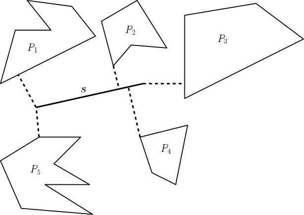
Obviously, if the query object intersects a polygon in then that polygon is a closest polygon and the closest distance from the query object to is zero. Following this observation, a query can be divided into two parts, executed in this order:
- 1.
Emptiness Query: Query if any polygon of is intersected by the query object. If there is such polygon, then report it as the answer, with a distance of zero.
- 2.
Proximity Query: (No polygon in S intersect the query object) Query for the closest polygon in .
Thus, one can separately develop data structures for the two steps above, aiming for the best trade-offs on preprocessing-space-query on both structures.
Emptiness queries have been addressed in the context of ray shooting among polygonal obstacles in the plane. Chazelle et al. [5] gave an algorithm for ray shooting queries among disjoint simple polygons with a total of edges, with preprocessing time, query time, and space. Obviously, ray shooting queries can be used to answer emptiness queries for both lines and line segments, within the same time and space bounds, by replacing each such query with two, respectively one, ray shooting queries.
Agarwal and Sharir [2] develop data structures for ray shooting queries by first building data structures for line and line segment intersection queries. They first address line intersection queries and show that a set of simple polygons with a total of vertices can be preprocessed in time into a data structure of size so that an intersection between a query line and the polygons can be detected on time. Alternately, they give a data structure with preprocessing time, space, and query time. When the query time becomes while when a query can be answered in time with space such that . For line segment intersection queries for disjoint simple polygons they give a data structure of size , that can be constructed in time and can answer whether a query segment intersects any of the polygons in time. Alternately, they gave a data structure with preprocessing time, space, and query time. For ray shooting among pairwise disjoint polygons, they give a data structure with preprocessing time, space, and query time.
We first warm up by providing a simple solution to finding the closest polygon to a query line in the following subsection. We then extend this approach to find the closest polygon to a query line segment.
2.1 Closest polygon to a query line
Given a set S of m disjoint simple polygons, with a total of vertices, to find the closest polygon to a query line we first perform an emptiness query with , as described earlier. Using the result in [2], this can be done with preprocessing time, space, and query time.
Given a simple polygon P and a line l such that l does not intersect P, the closest point of P from l is a vertex of P.
Assume that none of the polygons in intersect the query line . Based on Observation 2.1 to find the closest polygon in to the query line reduces to finding the closest point to a query line problem, where points corresponds to the vertices of the polygons in S. We further preprocess by computing the convex hull of each polygon in and taking the vertices of the convex hulls as the set of points. This requires only an additional time and storage. Thus, we have a set of points, where could be much smaller than in practice.
We can then use the results in [16, 14] for closest point to line queries. Putting things together we obtain the following result.
Lemma 1
A set S of polygons, with a total of vertices, can be preprocessed in time into a data structure of size , that can report the closest polygon to a query line in time, for arbitrary . Alternately, with time preprocessing one can construct a data structure of size that can report the closest polygon to a query line in time.
2.2 Closest polygon to a query line segment
Given a set S of m polygons, with a total of vertices, to find the closest polygon to a query line segment we first perform an emptiness query with . To facilitate that, we preprocess into a data structure for planar point location queries, which requires time and space [8]. Given a segment , we locate the endpoints of in this data structure, in query time; if any of the two endpoints is inside a polygon in then we are done.
If both endpoints of are in free space we proceed with a segment intersection query. As described earlier, this can be done with space, preprocessing time, and query time or, alternately, with query time, preprocessing time and space.
Assume that the line segment does not intersect any polygon in . Obviously, the closest distance from to is attained by a point on and a point on a line segment on the boundary of some polygon in .
Consider a line segment on the boundary of some polygon in . The closest distance between and is either along:
- 1.
A line perpendicular to and passing through an endpoint of , or
- 2.
A line perpendicular to and passing through an endpoint of , or
- 3.
A line joining an endpoint of and an endpoint of .
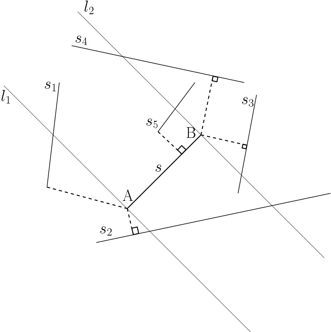
This is illustrated in Figure 3 where AB is the query segment and , and are five line segments (see also [19]). Lines and are perpendicular to segment and passing through points A and B, respectively.
Thus, we can focus on the line segments on the boundaries of the polygons in . Given a set of non-intersecting line segments, we want to build a data structure so that, for a query segment with endpoints and , the closest segment of can be quickly determined. From Observation 2.2, it is clear that the minimum distance involves an end point of at least one line segment. Therefore we can decompose this problem into the following two subproblems:
- 1.
Find the line segment of set closest to point or point .
- 2.
Let and be the lines perpendicular to at its endpoints and consider the endpoints of the line segments in M which lie between and . Find the closest such endpoint to .
Notice that for our purpose we could relax the second subproblem, and ask instead for finding the closest endpoint of to the query segment .
Subproblem 1: Given a set of line segments, preprocess so that we can efficiently find the closest line segment to a query point .
To answer Subproblem 1 we construct the Voronoi diagram of the line segments in and preprocess it for point location queries. Yap [21] provided an time algorithm to construct the Voronoi diagram of non intersecting line segments. After constructing the Voronoi diagram, preprocessing for point location takes time with storage, and a point location query can be answered in time [8].
Lemma 2
A set of non-intersecting line segments can be preprocessed in time into a data structure of size that can report the closest line segment to a query point in time.
For a given line segment , slab(s) is defined as the region bounded by the lines and perpendicular to the endpoints of and containing (see [4]).
Subproblem 2: Given a set of points, preprocess into a data structure so that one can efficiently answer the following query: For a line segment , find the closest point in to . This is illustrated in Figure 4.

To solve this problem, we use a multilevel data structure based on Matousek’s [11] decomposition scheme. Refer to Figure 4. Specifically, the first level is for halfplane range queries, to separates the points that are on the side of that contains , and the second level is for halfplane range queries on the resulting points to separate those that are on the side of and contain . These two levels are used to isolate the points in . The third level is for halfplane range queries bounded by the line supporting , to isolate the subsets of that are on either side of . The subsets on this level are further processed for closest point to line segment queries, when the query segment is outside the convex hull of the points, as in [4].
Using Theorem 6.1 from [11], we obtain the following trade-off.
Lemma 3
A set of points in the plane can be preprocessed in time and space into a data structure that can answer the query in Subproblem 2 in time, for any and .
Summing up, we have the following result.
Lemma 4
Given a set of disjoint simple polygons, it can be preprocessed in time into a data structure of size that can report the closest polygon in to a query line segment in time, for any and .
3 Closest polygon to path queries
We now turn our attention to finding the closest polygon to a query path. Given a set of disjoint simple polygons in the plane, with a total of vertices, we want to preprocess into a data structure so that for a query consisting of a positive constant and a simple polygonal path with vertices, from a point to a point in free space, one can quickly decide whether there is no polygonal obstacle within distance of .
Our solution actually works even if has self intersections, however we do not see the practical aspect of such paths.
To solve the path-polygons proximity query problem we proceed as follows.
Preprocessing. We build the following data structures.
- 1.
A point location data structure for the polygons is . It can be built with space and time, and can answer point location queries in time.
- 2.
A segment intersection data structure for the polygons of . As described earlier, this can be done with space, preprocessing time, and query time or, alternately, with query time, preprocessing time and space.
- 3.
The Voronoi diagram of the polygons in , enhanced with a point location data structure, . It can be built with space and time, and can answer point location and closest polygon to point queries in time.
- 4.
With the set of vertices of the polygons in , a data structure to find the closest point of to , for a query segment , as described in the previous section. It can be built with space and time, and can answer a query in time, for any and .
Query. Given a simple polygonal path with vertices, to answer a query we proceed as follows.
- 1.
Query with the vertices of . If any such vertex is inside some polygon of we stop and report it as the closest polygon to , with a zero distance (or an intersection flag). Otherwise, all vertices of are in free space and we proceed with the next step. This step takes time per query and thus time overall.
- 2.
Query with the line segments on . If it is found that a line segment intersects a polygon in then stop and report it as the closest polygon to , with a zero distance (or an intersection flag).
- 3.
Query with the vertices of and keep tract of the closest distance found. That distance gives the closest polygon of to the vertices of . This step takes time per query and thus time overall.
- 4.
Query to find the closest obstacle vertex in , for each segment of . This takes time per query and time overall, for any and .
Theorem 3.1
A set of disjoint simple polygons in the plane, with a total of vertices, can be preprocessed in time into a data structure of size so that given a query consisting of a positive value and a simple polygonal path with vertices one can answer if has clearance at least in time, for any and .
4 Conclusion and Extensions
In this paper, we studied the problem of finding the closest polygon of a set S of disjoint simple polygons to a query line segment or simple polygonal path. We proposed solutions that are significantly better in query time, when is small relative to , than what could be obtained from existing, non-query based approaches. Since queries with line segments along the query path are independent of each other, our result is easily parallelizable: with processors available, a query with a segment path would take time proportional to the time to answer a line segment query. When is small, this can be easily implemented by multithreading (JAVA, C++) on modern laptop and desktop computers.
A possible extension of our work, that we leave as an open problem, is to query with paths that are not polygonal, but formed of, or including, circular arcs. This version has direct applications in minimally invasive surgery, for instruments formed of circular tubes [15]. This problem seems significantly harder, even when the clearance (diameter of the tube) is known in advance. We sketch a possible approach here and underline the missing data structures needed to address this version.
It is easy to see that the minimum distance between a circular arc and a line segment could be achieved by a point and a point neither of which is an endpoint of or .
For the general version, with clearance given at query time one would need data structures for the following two types of queries: (1) circular arc intersection queries for disjoint polygons and (2) circular arc proximity queries for disjoint polygons. So far, neither of these data structures have been described in the computational geometry literature. There are however data structures for ray shooting queries among circular arcs [1], so if is comparable to one could instead answer ray shooting queries against at query time. Such method however seems inefficient.
Consider now the case when the clearance is known at preprocessing time. As before, we have a set of disjoint simple polygons in the plane, with a total of vertices. In addition, we also know the clearance , given as a positive real value. A query consists of a path with circular arcs and asks whether has clearance at least . To solve it, one can proceed as follows.
Preprocessing. Build the following data structures.
- 1.
Find the Minkowski sum of the obstacles in with a disk of radius and compute the union of the resulting objects, which can be done with space and time [19]. The boundary of consists of both line segments and circular arcs. Further process for point location queries, for an additional space and time. A point location query in the resulting data structure can be answered in time.
- 2.
Preporcess for circular ray shooting queries: given a circular arc determine the first line segment or arc on the boundary of hit by . Notice that the radius for the query circular arc is known in advance.
Thus, in this case, we are dealing only with a special case of circular ray shooting queries among disjoint line segments and circular arcs, where the radius of all circular arcs given at preprocessing time is the same. Still, we are not aware of any data structure that can efficiently handle such queries.
References
- [1] Agarwal, Pankaj K., Marc van Kreveld, and Mark Overmars. ”Intersection queries for curved objects.” Proceedings of the seventh annual symposium on Computational geometry. ACM, 1991.
- [2] Agarwal, Pankaj K., and Micha Sharir. ”Ray shooting amidst convex polygons in 2D.” Journal of Algorithms 21.3 (1996): 508-519.
- [3] Bespamyatnikh, Sergei. ”Computing closest points for segments.” International Journal of Computational Geometry Applications 13.05 (2003): 419-438.
- [4] Bespamyatnikh, Sergei, and Jack Snoeyink. ”Queries with segments in Voronoi diagrams.” Proceedings of the tenth annual ACM-SIAM symposium on Discrete algorithms. Society for Industrial and Applied Mathematics, 1999.
- [5] Chazelle, Bernard, et al. ”Ray shooting in polygons using geodesic triangulations.” Algorithmica 12.1 (1994): 54-68.
- [6] Cole, Richard, and Chee K. Yap. ”Geometric retrieval problems.” Foundations of Computer Science, 1983., 24th Annual Symposium on. IEEE, 1983.
- [7] Goswami, Partha P., Sandip Das, and Subhas C. Nandy. ”Triangular range counting query in 2D and its application in finding k nearest neighbors of a line segment.” Computational Geometry 29.3 (2004): 163-175.
- [8] Kirkpatrick, David. ”Optimal search in planar subdivisions.” SIAM Journal on Computing 12.1 (1983): 28-35.
- [9] Lee, D., Ching, Y., et al.: The power of geometric duality revisited. Info. Processing Letters 21 pp. 117–122 (1985)
- [10] Matousek, Jiri. ”Efficient partition trees.” Discrete Computational Geometry 8.3 (1992): 315-334.
- [11] Matousek, Jiri. ”Range searching with efficient hierarchical cuttings.” Discrete Computational Geometry 10.2 (1993): 157-182.
- [12] Mitchell, J.S.: Shortest paths among obstacles in the plane. International Journal of Computational Geometry Applications 6(03), 309–332 (1996)
- [13] Mitchell, J.S.: Geometric shortest paths and network optimization. Handbook of computational geometry 334, 633–702 (2000)
- [14] Mitra, P., Chaudhuri, B.: Efficiently computing the closest point to a query line1. Pattern Recognition Letters 19(11), 1027–1035 (1998)
- [15] Morimoto, T.K., Cerrolaza, J.J., Hsieh, M.H., Cleary, K., Okamura, A.M., Lingu- raru, M.G.: Design of patient-specific concentric tube robots using path planning from 3-d ultrasound. In: Engineering in Medicine and Biology Society (EMBC), 2017 39th Annual International Conference of the IEEE. pp. 165–168. IEEE (2017)
- [16] Mukhopadhyay, A.: Using simplicial partitions to determine a closest point to a query line. Pattern Recognition Letters 24(12), 1915–1920 (2003)
- [17] Segal, M., Zeitlin, E.: Computing closest and farthest points for a query segment. Theoretical Computer Science 393(1-3), 294–300 (2008)
- [18] Storer, J.A., Reif, J.H.: Shortest paths in the plane with polygonal obstacles. Jour- nal of the ACM (JACM) 41(5), 982–1012 (1994)
- [19] Wein, R., Van Den Berg, J., Halperin, D.: Planning high-quality paths and corri- dors amidst obstacles. The International Journal of Robotics Research 27(11-12), 1213–1231 (2008)
- [20] Weina, R., van den Bergb, J.P., Halperina, D.: The visibility–voronoi complex and its applications. Computational Geometry 36, 66–87 (2007)
- [21] Yap, C.K.: Ano (n logn) algorithm for the voronoi diagram of a set of simple curve segments. Discrete Computational Geometry 2(4), 365–393 (1987)