On sampling from a log-concave density using kinetic Langevin diffusions

Markov processes and, more particularly, diffusion processes are often used in order to solve the problem of sampling from a given density $\pi$. This problem can be formulated as follows. Assume that we are able to generate an arbitrary number of independent standard Gaussian random variables $\xi_{1},\ldots,\xi_{K}$. For a given precision level $\varepsilon>0$ and a given metric $d$ on the space of probability measures, the goal is to devise a function $F_{\varepsilon}$ such that the distribution $\nu_{K}$ of the random variable $\vartheta_{K}=F_{\varepsilon}(\xi_{1},\ldots,\xi_{K})$ satisfies $d(\mu_{K},\pi)\leq\varepsilon$. For solving this task, it is often assumed that we can have access to the evaluations of the probability density function of $\pi$ as well as its derivatives. Among different functions $F_{\varepsilon}$ having the aforementioned property, the most interesting are those that require the smallest number of computations.

Markov Chain Monte Carlo methods hinge on random variables $\vartheta_{K}$ and associated functions $F_{\varepsilon}$ defined by recursion $\vartheta_{k}=G_{\varepsilon}(\vartheta_{k-1},\xi_{k})$, $k=1,\ldots,K$, where $G_{\varepsilon}$ is some function of two arguments. For a given target distribution $\pi$, if one succeeds to design a function $G_{\varepsilon}$ such that the Markov process $\{\vartheta_{k};k\in\mathbb{N}\}$ is ergodic with invariant density $\pi$ then, for large $K$, the distribution of $\vartheta_{K}$ will be close to $\pi$. Therefore, if the evaluation of $G_{\varepsilon}$ involves only simple operations, we get a solution of the task of approximate sampling from $\pi$. Of course, it is important to address the problem of the choice of the number of iterations $K$ ensuring that the sampling error is smaller than $\varepsilon$. However, it is even more important to be able to design functions $G_{\varepsilon}$, often referred to as the update rule, with desired properties presented above.

Discretization of continuous-time Markov processes is a successful generic method for defining update rules. The idea is to start by specifying a continuous-time Markov process, $\{L_{t}:t\geq 0\}$, which is provably positive recurrent and has the target $\pi$ as invariant distribution¹¹ 1 More generally, one can consider a Markov process having an invariant distribution that is close to $\pi$. . The second step is to set-up a suitable time-discretization of the continuous-time process. More precisely, since $\{L_{t}\}$ is a Markov process, for any step-size $h>0$, there is a mapping $G$ such that $L_{kh}\stackrel{{\scriptstyle\mathscr{D}}}{{=}}G(L_{(k-1)h},\xi_{k})$, $k=1,\ldots,K$, where $\xi_{k}$ is a standard Gaussian random variable independent of $L_{(k-1)h}$. This mapping $G$ might not be available in a closed form. Therefore, the last step is to approximate $G$ by a tractable mapping $G_{\varepsilon}$. Langevin diffusions are a class of continuous-time Markov processes for which the invariant density is available in closed-form. For this reason, they are suitable candidates for applying the generic approach of the previous paragraph.

Let $m$ and $M$ be two positive constants such that $m\leq M$. Throughout this work, we will assume that the target distribution $\pi$ has a density with respect to the Lebesgue measure on $\mathbb{R}^{p}$, which is of the form $\pi(\boldsymbol{\theta})=Ce^{-f(\boldsymbol{\theta})}$ for a function $f$ that is $m$-strongly convex and with an $M$-Lipschitz gradient. The (highly overdamped) Langevin diffusion having $\pi$ as invariant distribution is defined as a strong solution to the stochastic differential equation

where $\boldsymbol{W}$ is a $p$-dimensional standard Brownian motion. The update rule associated to this process, obtained by using the Euler discretization, is given by the equation $G_{\varepsilon}(\boldsymbol{L}_{(k-1)h},\boldsymbol{\xi}_{k})=-h\nabla f(\boldsymbol{L}_{(k-1)h})+\sqrt{2h}\,\boldsymbol{\xi}_{k}$ with $\boldsymbol{\xi}_{k}\stackrel{{\scriptstyle\mathscr{D}}}{{=}}h^{-1/2}(\boldsymbol{W}_{kh}-\boldsymbol{W}_{(k-1)h})$ being a $p$-dimension standard Gaussian vector. The resulting approximate sampling method is often called Langevin Monte Carlo (LMC) or Unadjusted Langevin Algorithm (ULA). Its update rule follows from (2) by replacing the function $t\mapsto\nabla f(\boldsymbol{L}_{t})$ by its piecewise constant approximation. Therefore, the behavior of the LMC is governed by the following two characteristics of the continuous-time process: the mixing rate and the smoothness of the sample paths. A quantitative bound on the mixing rate allows us to choose a time horizon $T$ such that the distribution of the random vector $\boldsymbol{L}_{T}$ is within a distance $\varepsilon/2$ of the target distribution, whereas the smoothness of sample paths helps us to design a step-size $h$ so that the distribution of the discretized process at $K=T/h$ is within a distance $\varepsilon/2$ of the distribution of $\boldsymbol{L}_{T}$. For the LMC, we know that the Langevin diffusion mixes exponentially fast with the precise rate $e^{-mt}$. In addition, almost all sample paths of $\boldsymbol{L}$ are Hölder continuous of degree $\alpha$, for every $\alpha<1/2$. Combining these properties, it has been shown that it suffices $K_{\varepsilon}=O((p/\varepsilon^{2})\log(p/\varepsilon^{2}))$ iterations for the LMC algorithm to achieve an error smaller than $\varepsilon$ (both in total-variation and Wasserstein distances); see (Dalalyan, 2017b) for the first nonasymptotic result of this type and (Durmus and Moulines, 2016; Durmus and Moulines, 2017; Dalalyan and Karagulyan, 2017) for improved versions of it.

Under the same assumptions on the log-target $f$, one can consider the kinetic Langevin diffusion, also known as the second-order Langevin process, defined by

where $\gamma>0$ is the friction coefficient and $u>0$ is the inverse mass. As proved in (Nelson, 1967, Theorem 10.1), the highly overdamped Langevin diffusion (2) is obtained as a limit of the rescaled kinetic diffusion $\bar{\boldsymbol{L}}_{t}=\boldsymbol{L}_{\gamma t}$, where $\boldsymbol{L}$ is defined as in (3) with $u=1$, when the friction coefficient $\gamma$ tends to infinity.

The continuous-time Markov process $(\boldsymbol{L}_{t},\boldsymbol{V}_{t})$ is positive recurrent and its invariant distribution is absolutely continuous with respect to the Lebesgue measure on $\mathbb{R}^{2p}$. The corresponding invariant density is given by

This means that under the invariant distribution, the components $\boldsymbol{L}$ and $\boldsymbol{V}$ are independent, $\boldsymbol{L}$ is distributed according to the target $\pi$, whereas $\boldsymbol{V}/\sqrt{u}$ is a standard Gaussian vector. Therefore, one can use this process for solving the problem of sampling from $\pi$. As discussed above, the quality of the resulting sampler will depend on two key properties of the process: rate of mixing and smoothness of sample paths. The rate of mixing of kinetic diffusions has been recently studied by Eberle et al. (2017) under conditions that are more general than strong convexity of $f$. In strongly convex case, a more tractable result has been obtained by Cheng et al. (2017). It establishes that for $\gamma=2$ and $u=1/M$, the mixing rate in the Wasserstein distance is $e^{-(m/2M)t}$; see Theorem 5 in (Cheng et al., 2017). On the other hand, sample paths of the process $\{\boldsymbol{L}\}$ defined in (3) are smooth of order $1+\alpha$, for every $\alpha\in[0,1/2[$. Combining these two properties, (Cheng et al., 2017) prove that a suitable discretization of (3) leads to a sampler that achieves an error smaller than $\varepsilon$ in a number of iterations $K$ satisfying $K=O((p/\varepsilon^{2})^{1/2}\log(p/\varepsilon))$.

It follows from the discussion of previous paragraphs that the kinetic LMC based on (3) converges faster than the standard LMC based on (2). Furthermore, this improved rate of convergence is mainly due to the higher smoothness of sample paths of the underlying Markov process. The main purpose of the present work is to pursue the investigation of the kinetic Langevin Monte Carlo (KLMC) initiated in (Cheng et al., 2017) by addressing the following questions:

• Q1.

  What is the rate of mixing of the continuous-time kinetic Langevin diffusion for general values of the parameters $u$ and $\gamma$?

• Q2.

  Is it possible to improve the rate of convergence of the KLMC by optimizing it over the choice of $u$, $\gamma$ and the step-size ?

• Q3.

  If the function $f$ happens to have a Lipschitz-continuous Hessian, is it possible to devise a discretization that takes advantage of this additional smoothness and leads to improved rates of convergence?

The rest of the paper is devoted to answering these questions. The rate of mixing for the continuous-time process is discussed in Section 2. In a nutshell, we show that if $\gamma\geq\sqrt{(M+m)u}$, then the rate of mixing is of order $e^{-(um/\gamma)t}$. Non-asymptotic guarantees for the KLMC algorithm are stated and discussed in Section 3. They are in the same spirit as those established in (Cheng et al., 2017), but have an improved dependence on the condition number, the ratio of the Lipschitz constant $M$ and the strong convexity constant $m$. Our result has also improved constants and is much less sensitive to the choice of the initial distribution. These improvements are achieved thanks to a more careful analysis of the discretization error of the Langevin process. Finally, we present in Section 4 a new discretization, termed second-order KLMC, of the kinetic Langevin diffusion that exploits the knowledge of the Hessian of $f$. Its error, measured in the Wasserstein distance $W_{2}$ is shown to be bounded by $\varepsilon$ for a number of iterations that scales as $(p/\varepsilon)^{1/2}$. Thus, we get an improvement of order $(1/\varepsilon)^{1/2}$ over the first-order KLMC algorithm.

Let us denote by $\mathbf{P}_{t}^{\boldsymbol{L}}$ the transition probability at time $t$ of the kinetic diffusion $\boldsymbol{L}$ defined by (3). This means that $\mathbf{P}_{t}^{\boldsymbol{L}}$ is a Markov kernel given by $\mathbf{P}_{t}^{\boldsymbol{L}}((\boldsymbol{x},\boldsymbol{v}),B)=\mathbf{P}(\boldsymbol{L}_{t}\in B|\boldsymbol{V}_{0}=\boldsymbol{v},\boldsymbol{L}_{0}=\boldsymbol{x})$, for every $\boldsymbol{v},\boldsymbol{x}\in\mathbb{R}^{p}$ and any Borel set $B\subset\mathbb{R}^{p}$. For any probability distribution $\mu$ on $\mathbb{R}^{p}\times\mathbb{R}^{p}$, we denote $\mu\mathbf{P}_{t}^{\boldsymbol{L}}$ the (unconditional) distribution of the random variable $\boldsymbol{L}_{t}$ when the starting distribution of the process $(\boldsymbol{V},\boldsymbol{L})$ is $\mu$ (i.e., when $(\boldsymbol{V},\boldsymbol{L}_{0})\sim\mu$).

Since the process $(\boldsymbol{V},\boldsymbol{L})$ is ergodic, whatever the initial distribution, for large values of $t$ the distribution of $\boldsymbol{L}_{t}$ is close to the invariant distribution. We want to quantify how fast does this convergence occur. Furthermore, we are interested in a nonasymptotic result in the Wasserstein-Kantorovich distance $W_{2}$, valid for a large set of possible values $(\gamma,u)$.

A first observation is that, without loss of generality, we can focus our attention to the case $u=1$. This is made formal in the next lemma.

The proof of this result is straightforward and therefore is omitted. Note that it shows that the parameter $u$ merely represents a time scale (the speed of running over the path of the process $\boldsymbol{L}$). Therefore, in the rest of this paper, we will consider the parameter $u$ to be equal to 1.

The proof of this result is postponed to Section 7. Here, we will discuss some consequences of it and present the main ingredient of the proof. First of all, note that this result implies that for $\gamma^{2}>2\vee M$, the operator $\mathbf{P}_{t}^{\boldsymbol{L}}$ is a contraction. The rate of this contraction is characterized by the parameter $\beta$. If we optimize the exponent in (6) with respect to $v$, we get the optimal rates of contraction reported in Table 1.

If we consider the case $\gamma=2\sqrt{Mu}=2\sqrt{M}$ previously studied in (Cheng et al., 2017), then the best rate of contraction provided by (6) corresponds to $v=\sqrt{M}-\sqrt{M-m}$, and the upper bound of Theorem 1 reads as

One can check that the constant $\sqrt{M}-\sqrt{M-m}$ that we obtain within the exponential is optimal, in the sense that one gets exactly this constant in the case where $f$ is the bivariate quadratic function $f(x_{1},x_{2})=(m/2)x_{1}^{2}+(M/2)x_{2}^{2}$. This constant is slightly better than the one obtained in (Cheng et al., 2017, Lemma 8) for the particular choice of the time scale $u=1/M$. Indeed, if we rewrite the two results in the common time-scale $u=1$, (Cheng et al., 2017, Lemma 8) provides the contraction rate $\beta=m/(2\sqrt{M})$, which is smaller than (but asymptotically equivalent to) $\sqrt{M}-\sqrt{M-m}$.

Another relevant consequence is obtained by instantiating (5) to the case $\gamma\geq\sqrt{M+m}$. This leads to the bound

This result is interesting since it allows to optimize the argument of the exponent with respect to $\gamma$ for fixed $t$. The corresponding optimized constant is $m/\sqrt{M+m}$, which improves on the constant obtained in (7) for $\gamma=2\sqrt{M}$. When $M/m$ becomes large, the improvement factor gets close to 2.

We now describe the main steps of the proof of Theorem 1. The main idea is to consider along with the process $(\boldsymbol{V},\boldsymbol{L})$, another process $(\boldsymbol{V}^{\prime},\boldsymbol{L}^{\prime})$ that satisfies the same SDE (3) as $(\boldsymbol{V},\boldsymbol{L})$, with the same Brownian motion but with different initial conditions. One easily checks that

Using the mean value theorem, we infer that for a suitable symmetric matrix $\mathbf{H}_{t}$, we have $\nabla f(\boldsymbol{L}_{t})-\nabla f(\boldsymbol{L}^{\prime}_{t})=\mathbf{H}_{t}(\boldsymbol{L}_{t}-\boldsymbol{L}^{\prime}_{t})$. Furthermore, $\mathbf{H}_{t}$ being the Hessian of a strongly convex function satisfies $\mathbf{H}_{t}\succeq m\mathbf{I}_{p}$. Then, (9) can be rewritten as

In a small neighborhood of any fixed time instance $t_{0}$, (10) is close to a linear differential equation with the associated matrix

It is well-known that the solution of such a differential equation will tend to zero if and only if the real parts of all the eigenvalues of $\mathbf{M}(t_{0})$ are negative. The matrix $\mathbf{M}(t_{0})$ is not symmetric; it is in most cases diagonalizable but its eigenvectors generally depend on $t_{0}$. To circumvent this difficulty, we determine the transformations diagonalizing the surrogate matrix

This yields an invertible matrix $\mathbf{P}$ such that $\mathbf{P}^{-1}\mathbf{M}\mathbf{P}$ is diagonal. We can thus rewrite (10) in the form

Interestingly, we prove that the quadratic form associated with the matrix $\mathbf{P}^{-1}\mathbf{M}(t)\mathbf{P}$ is negative definite and this provides the desired result. Furthermore, we use this same matrix $\mathbf{P}$ for analyzing the discretized version of the kinetic Langevin diffusion and proving the main result of the next section.

Let us start this section by recalling the KLMC algorithm, the sampler derived from a suitable time-discretization of the kinetic diffusion, introduced by Cheng et al. (2017). Let us define the sequence of functions $\psi_{k}$ by $\psi_{0}(t)=e^{-\gamma t}$ and $\psi_{k+1}(t)=\int_{0}^{t}\psi_{k}(s)\,ds$. Recall that $f$ is assumed twice differentiable and, without loss of generality, the parameter $u$ is assumed to be equal to one. The discretization involves a step-size $h>0$ and is defined by the following recursion:

where $(\boldsymbol{\xi}_{k+1},\boldsymbol{\xi}^{\prime}_{k+1})$ is a $2p$-dimensional centered Gaussian vector satisfying the following conditions:

• •

  $(\boldsymbol{\xi}_{j},\boldsymbol{\xi}^{\prime}_{j})$’s are iid and independent of the initial condition $(\boldsymbol{v}_{0},\boldsymbol{\vartheta}_{0})$,

• •

  for any fixed $j$, the random vectors $\big((\boldsymbol{\xi}_{j})_{1},(\boldsymbol{\xi}^{\prime}_{j})_{1}\big)$, $\big((\boldsymbol{\xi}_{j})_{2},(\boldsymbol{\xi}^{\prime}_{j})_{2}\big)$, $\ldots$, $\big((\boldsymbol{\xi}_{j})_{p},(\boldsymbol{\xi}^{\prime}_{j})_{p}\big)$ are iid with the covariance matrix

  $$\mathbf{C}=\int_{0}^{h}[\psi_{0}(t)\ \psi_{1}(t)]^{\top}[\psi_{0}(t)\ \psi_{1}(t)]\,dt.$$

This recursion may appear surprizing, but one can check that it is obtained by first replacing in (3), on each time interval $t\in[kh,(k+1)h]$, the gradient $\nabla f(\boldsymbol{L}_{t})$ by $\nabla f(\boldsymbol{L}_{kh})$, by renaming $(\boldsymbol{V}_{kh},\boldsymbol{L}_{kh})$ into $(\boldsymbol{v}_{k},\boldsymbol{\vartheta}_{k})$ and by explicitly solving the obtained linear SDE (which leads to an Ornstein-Uhlenbeck process). To the best of our knowledge, the algorithm (12), that we will refer to as KLMC, has been first proposed by Cheng et al. (2017). The next result characterizes its approximation properties.

The proof of this theorem, postponed to Section 8, is inspired by the proof in (Cheng et al., 2017), but with a better control of the discretization error. This allows us to achieve the following improvements as compared to aforementioned paper:

• •

  The second term in the upper bound provided by Theorem 2 scales linearly as a function of the condition number $\varkappa\triangleq M/m$, whereas the corresponding term in (Cheng et al., 2017) scales as $\varkappa^{3/2}$.

• •

  The impact of the initial distribution $\nu_{0}$ on the overall error of sampling appears only in the first term, which is multiplied by a sequence that has an exponential decay in $k$. As a consequence, if we denote by $K$ the number of iterations sufficient for the error to be smaller than a prescribed level $\varepsilon$, our result leads to an expression of $K$ in which $W_{2}(\nu_{0},\pi)$ is within a logarithm. Recall that the expression of $K$ in (Cheng et al., 2017, Theorem 1) scales linearly in $W_{2}(\nu_{0},\pi)$.

• •

  The numerical constants of Theorem 2 are much smaller than those of the corresponding result in (Cheng et al., 2017).

In order to ease the comparison of our result to (Cheng et al., 2017, Theorem 1), let us apply Theorem 2 to

and $\gamma=\sqrt{m+M}$, which corresponds to the tightest upper bound furnished by our theorem. Note that in (Cheng et al., 2017) it is implicitly assumed that $p/\varepsilon^{2}$ is large enough so that the second term in the minimum appearing in (14) is smaller than the first term. From (14) we obtain that³³ 3 This value of $K$ is obtained by choosing $h$ and $K$ so that the second term in the upper bound of Theorem 2 is equal to $(1-\sqrt{2}/24)\epsilon$ whereas the first term is smaller than $(\sqrt{2}/24)\epsilon$.

iterations are sufficient for having $W_{2}(\nu_{K},\pi)\leq\varepsilon$. After some simplifications, we get

Remind that the corresponding result in Cheng et al. (2017) requires $K$ to satisfy⁴⁴ 4 This lower bound on $K$ is obtained by replacing $\mathcal{D}^{2}\triangleq\|\boldsymbol{\theta}_{0}-\boldsymbol{\theta}^{*}\|_{2}$ by 0 in (Cheng et al., 2017, Theorem 1).

Thus, the improvement in terms of the number of iterations we obtain is at least by a factor $17\sqrt{\varkappa}$, whenever $\kappa\leq p/(16m\varepsilon^{2})$.

It is also helpful to compare the obtained result (16) to the analogous result for the highly overdamped Langevin diffusion (Durmus and Moulines, 2016). Using (Durmus et al., 2018, Eq. (22)), one can check that this is enough to choose an integer

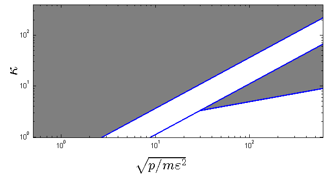
such that $K_{\rm LMC}$ iterations of the LMC algorithm are sufficient to arrive at an error bounded by $\varepsilon$. Comparing (16) and (18), we see that the KLMC is preferable to the LMC when $p/(m\varepsilon^{2})$ is large as compared to the condition number $\varkappa$. This is typically the case when the dimensionality is high or a high precision approximation is required. The order of preference is reversed when the condition number $\varkappa$ is large as compared to $p/(m\varepsilon^{2})$. Such a situation corresponds to settings where the target log-density $f$ is nearly flat ($m$ is small) or has a gradient that may increase very fast ($M$ is large). As an important conclusion, we can note that none of these two methods is superior to the other in general. The plot in Figure 1 illustrates this fact by showing in gray the regions where LMC outperforms KLMC.

In this section, we propose another discretization of the kinetic Langevin process, which is applicable when the function $f$ is twice differentiable. We show below that this new discretization leads to a provably better sampling error under the condition that the Hessian matrix of $f$ is Lipschitz-continuous with respect to the spectral norm. At any iteration $k\in\mathbb{N}$, we define $\mathbf{H}_{k}=\nabla^{2}f(\boldsymbol{\vartheta}_{k})$ and

where

• •

  $\psi_{0},\psi_{1},\psi_{2}$ are defined as in the beginning of the previous section,

• •

  $\varphi_{k+1}(t)=\int_{0}^{t}e^{-\gamma(t-s)}\psi_{k}(s)\,ds$ for every $t>0$,

• •

  the $4p$ dimensional random vectors $(\boldsymbol{\xi}_{k+1}^{(1)},\boldsymbol{\xi}_{k+1}^{(2)},\boldsymbol{\xi}_{k+1}^{(3)},\boldsymbol{\xi}_{k+1}^{(4)})$ are iid Gaussian with zero mean,

• •

  for any fixed $j$, the $4$-dimensional random vectors $\big([(\boldsymbol{\xi}_{j}^{(1)})_{1},(\boldsymbol{\xi}_{j}^{(2)})_{1},(\boldsymbol{\xi}_{j}^{(3)})_{1},(\boldsymbol{\xi}_{j}^{(4)})_{1}]$, $\ldots$,
  $[(\boldsymbol{\xi}_{j}^{(1)})_{p},(\boldsymbol{\xi}_{j}^{(2)})_{p},(\boldsymbol{\xi}_{j}^{(3)})_{p},(\boldsymbol{\xi}_{j}^{(4)})_{p}]\big)$ are iid with the covariance matrix

  (20)

  $\displaystyle\bar{\mathbf{C}}=\int_{0}^{h}[\psi_{0}(t);\,\psi_{1}(t);\,\varphi_{2}(t);\,\varphi_{3}(t)]^{\top}[\psi_{0}(t);\,\psi_{1}(t);\,\varphi_{2}(t);\,\varphi_{3}(t)]\,dt.$

This definition is somewhat complicated, but it follows from an application of the second-order Taylor approximation to the drift term of the kinetic Langevin diffusion⁵⁵ 5 For more detailed explanations, see Section 9.1. At this stage, one can note that if the Hessian $\mathbf{H}_{k}$ is zero, then the update rule (19) boils down to the update rule of the KLMC algorithm in (12). Iterating the update rule (19) we get a random variable that will be henceforth called KLMC2 or second-order kinetic Langevin Monte-Carlo algorithm.

Several important consequences can be drawn from this result. First, the value of the parameter $\gamma$ minimizing the right hand side is its smallest possible value $\gamma=\sqrt{m+M}$. Second, one can note that the last term of the obtained upper bound is independent of dimension $p$ and decreases exponentially fast in $1/h$. This term is in most cases negligible with respect to the other terms involved in the upper bound. In particular, we deduce from this result that if the Lipschitz constants $M$ and $M_{2}$ are bounded and the strong convexity constant $m$ is bounded away from zero, then the KLMC2 algorithm achieves the precision level $\varepsilon$ after $K_{\varepsilon}$ iterations, with $K_{\varepsilon}$ being of order $\sqrt{p/\varepsilon}$, up to a logarithmic factor. Finally, if we neglect the last term in the upper bound of Theorem 3, and choose the parameters $h$ and $k$ so that the other terms are equal to $\varepsilon/\sqrt{4m}$, we get that the number of iteration $K_{\varepsilon}$ to achieve an error $\varepsilon/\sqrt{m}$ scales, up to a logarithmic factor, as $\sqrt{M}/(mh_{\varepsilon})=\sqrt{p}\,\varkappa_{2}^{2}+\sqrt{p/\varepsilon}\,\varkappa_{2}^{5/4}$, where $\varkappa_{2}=(M_{2}^{2/3}+Mp^{-1/3})/m$ is a version of the condition number taking into account the Hessian-Lipschitz assumption.

It is interesting to compare this result to the convergence result for the LMCO algorithm established in (Dalalyan and Karagulyan, 2017). We can note that the number of iterations that are sufficient for the KLMC2 to achieve the error $\varepsilon$ is much smaller than the corresponding number for the LMCO: $\sqrt{p/\varepsilon}$ versus $p/\varepsilon$. In addition, the KLMC2 algorithm does not need to compute matrix exponentials neither to do matrix inversion. The most costly operations are that of computing the products of the $p\times p$ Hessian and the vectors $\boldsymbol{v}_{k}$, $\boldsymbol{\xi}_{k+1}^{3}$ and $\boldsymbol{\xi}_{k+1}^{3}$. In most cases, the complexity of these computations scales linearly in $p$.

As a conclusion, to the best of our knowledge, the second-order KLMC algorithm provides the best known convergence rate $\sqrt{p/\varepsilon}$ for a target density $\pi$ having a log-density that is concave and Hessian-Lipschitz.

The idea of using the Langevin diffusion (see (Pavliotis, 2014) for an introduction to this topic) for approximating a random variable drawn from its invariant distribution is quite old and can be traced back at least to (Roberts and Tweedie, 1996). Since then, many papers focused on analyzing the asymptotic behavior of the Langevin-based methods under various assumptions, see (Lamberton and Pagès, 2003; Lamberton and Pagès, 2002; Stramer and Tweedie, 1999a; Stramer and Tweedie, 1999b; Douc et al., 2004; Pillai et al., 2012; Xifara et al., 2014; Roberts and Stramer, 2002; Roberts and Rosenthal, 1998; Bou-Rabee and Hairer, 2013) and the references therein. Convergence to the invariant distribution for Langevin processes is studied in (Desvillettes and Villani, 2001; Helffer and Nier, 2005; Dolbeault et al., 2015).

Non-asymptotic and computable bounds on the convergence to equilibrium of the kinetic Langevin diffusion have been recently obtained in (Eberle et al., 2017; Cheng et al., 2018; Cheng et al., 2017). While (Cheng et al., 2017) considers only the convex case, (Eberle et al., 2017; Cheng et al., 2018) deal also with nonconvexity. On the one hand, (Cheng et al., 2018) provide results only for a fixed value of parameters $(\gamma,u)=(2,1/M)$. On the other hand, if we instantiate results of (Eberle et al., 2017) to the case of convex functions $f$, convergence to the invariant density is proved under the condition $\gamma^{2}\geq 30Mu$. This is to be compared to the conditions of Theorem 1 that establishes exponential convergence as soon as $\gamma^{2}>Mu$.

Nonasymptotic bounds on the precision of the Langevin Monte Carlo under strong convexity have been established in (Dalalyan, 2017b) and then extended and refined in a series of papers (Durmus and Moulines, 2016; Bubeck et al., 2015; Dalalyan, 2017a; Cheng and Bartlett, 2017; Durmus and Moulines, 2017; Brosse et al., 2017; Durmus et al., 2018; Luu et al., 2017; Bernton, 2018). Very recently, it was proved in (Dwivedi et al., 2018) that applying a Metropolis-Hastings correction to the LMC leads to improved dependence on the target precision $\epsilon$ of the number of gradient evaluations. The fact that the discretized version of the kinetic Langevin diffusion may outperform its highly overdamped counterpart was observed and quantified in (Cheng et al., 2017).

Previous work has also studied the precision of Langevin algorithms in the case when the gradient evaluations are contaminated by some noise (Dalalyan, 2017a; Dalalyan and Karagulyan, 2017; Cheng et al., 2017; Baker et al., 2018; Chatterji et al., 2018) and the relation with stochastic optimization (Raginsky et al., 2017; Zhang et al., 2017; Xu et al., 2017; Dieuleveut et al., 2017). There are certainly many other papers related to the present work that are not mentioned in this section. There is a vast literature on this topic and it will be impossible to quote all the papers. We believe that the papers cited here and the references therein provide a good overview of the state of the art.

In order to summarize the content of the previous sections, let us return, on by one, to the questions raised in the introduction. First, concerning the mixing properties of the kinetic Langevin diffusion for general values of $u$ and $\gamma$, we have established that as soon as $\gamma^{2}>Mu$, the process mixes exponentially fast with a rate at least equal to $\{mu\wedge(\gamma^{2}-Mu)\}/\gamma$. Therefore, for fixed values of $m$, $M$ and $u$, the nearly fastest rate of mixing is obtained for $\gamma^{2}=(m+M)u$ and is equal to $m/\sqrt{m+M}$.

To answer the second question, we have seen that optimization with respect to $\gamma$ and $u$ leads to improved constants but does not improve the rate. Indeed, if we use the values of $\gamma$ and $u$ used in (Cheng et al., 2017) (that is $\gamma=2$ and $u=1/M$, which in view of Lemma 1 are equivalent to $\gamma=2\sqrt{M}$ and $u=1$) lead to a bound on the number of iterates sufficient to achieve a precision $\varepsilon$ that is of the same order as the optimized one given in (15). Interestingly, our analysis revealed that not only the numerical constants of the result in (Cheng et al., 2017) can be improved, but also the dependence on the condition number $\varkappa=M/m$ can be made better. Indeed, we have managed to replace the factor $\varkappa^{2}$ by $\varkappa^{3/2}$. Such an improvement might have important consequences in generalizing the results to the case of a convex function which is not strongly convex. This line of research will be explored in a future work. Our bound exhibits also a better dependence on the error of the first step: it is logarithmic in our result while it was linear in (Cheng et al., 2017).

Finally, we have given an affirmative answer to the third question. We have shown that leveraging second-order information may reduce the number of steps of the algorithm by a factor proportional to $1/\sqrt{\varepsilon}$, where $\varepsilon$ is the target precision. In order to better situate this improvement in the context of prior work, the table below reports the order of magnitude of the number of steps⁷⁷ 7 To ease the comparison, we consider $\varkappa$ as a fixed constant and do not report the dependence on $\varkappa$ in this table. of Langevin related algorithms in the strongly convex case:

This section is devoted to proofs of the results stated in Section 2. Let $\boldsymbol{L}_{0},\boldsymbol{L}_{0}^{\prime}$ and $\boldsymbol{V}_{0}$ be three $p$-dimensional random vectors defined on the same probability space such that

• •

  $\boldsymbol{V}_{0}$ is independent of $(\boldsymbol{L}_{0},\boldsymbol{L}_{0}^{\prime})$,

• •

  $\boldsymbol{V}_{0}\sim\mu_{1}$, whereas $\boldsymbol{L}_{0}\sim\mu_{2}$ and $\boldsymbol{L}^{\prime}_{0}\sim\mu_{2}^{\prime}$,

• •

  $W_{2}^{2}(\mu_{2},\mu_{2}^{\prime})=\mathbf{E}[\|\boldsymbol{L}_{0}-\boldsymbol{L}_{0}^{\prime}\|_{2}^{2}]$.

Let $\boldsymbol{W}$ be a Brownian motion on the same probability space. We define $(\boldsymbol{V},\boldsymbol{L})$ and $(\boldsymbol{V}^{\prime},\boldsymbol{L}^{\prime})$ as kinetic Langevin diffusion processes driven by the same Brownian motion $\boldsymbol{W}$ and satisfying the initial condition $\boldsymbol{V}^{\prime}_{0}=\boldsymbol{V}_{0}$. From the definition of the Wasserstein distance, it follows that

In view of this inequality, it suffices to find an appropriate upper bound on the right hand side of the last display, in order to prove Theorem 1. This upper bound is provided below in Proposition 1.

References

• Baker et al. (2018) Baker, J., Fearnhead, P., Fox, E. B., and Nemeth, C. (2018). Control variates for stochastic gradient mcmc. Statistics and Computing.
• Bernton (2018) Bernton, E. (2018). Langevin Monte Carlo and JKO splitting. In Bubeck, S., Perchet, V., and Rigollet, P., editors, Proceedings of the 31st Conference On Learning Theory, volume 75 of Proceedings of Machine Learning Research, pages 1777–1798.
• Bou-Rabee and Hairer (2013) Bou-Rabee, N. and Hairer, M. (2013). Nonasymptotic mixing of the MALA algorithm. IMA J. Numer. Anal., 33(1):80–110.
• Brosse et al. (2017) Brosse, N., Durmus, A., Moulines, E., and Pereyra, M. (2017). Sampling from a log-concave distribution with compact support with proximal langevin monte carlo. In Kale, S. and Shamir, O., editors, Proceedings of the 2017 Conference on Learning Theory, volume 65 of Proceedings of Machine Learning Research, pages 319–342, Amsterdam, Netherlands.
• Bubeck et al. (2015) Bubeck, S., Eldan, R., and Lehec, J. (2015). Sampling from a log-concave distribution with Projected Langevin Monte Carlo. ArXiv e-prints.
• Chatterji et al. (2018) Chatterji, N., Flammarion, N., Ma, Y., Bartlett, P., and Jordan, M. (2018). On the theory of variance reduction for stochastic gradient Monte Carlo. In Dy, J. and Krause, A., editors, Proceedings of the 35th International Conference on Machine Learning, volume 80 of Proceedings of Machine Learning Research, pages 764–773, Stockholmsmassan, Stockholm Sweden.
• Cheng and Bartlett (2017) Cheng, X. and Bartlett, P. (2017). Convergence of Langevin MCMC in KL-divergence. ArXiv e-prints.
• Cheng et al. (2018) Cheng, X., Chatterji, N. S., Abbasi-Yadkori, Y., Bartlett, P. L., and Jordan, M. I. (2018). Sharp Convergence Rates for Langevin Dynamics in the Nonconvex Setting. ArXiv e-prints.
• Cheng et al. (2017) Cheng, X., Chatterji, N. S., Bartlett, P. L., and Jordan, M. I. (2017). Underdamped Langevin MCMC: A non-asymptotic analysis. ArXiv e-prints.
• Collier and Dalalyan (2017) Collier, O. and Dalalyan, A. S. (2017). Minimax estimation of a p-dimensional linear functional in sparse gaussian models and robust estimation of the mean. submitted 1712.05495, arXiv.
• Dalalyan (2017a) Dalalyan, A. (2017a). Further and stronger analogy between sampling and optimization: Langevin monte carlo and gradient descent. In Kale, S. and Shamir, O., editors, Proceedings of the 2017 Conference on Learning Theory, volume 65 of Proceedings of Machine Learning Research, pages 678–689.
• Dalalyan (2017b) Dalalyan, A. S. (2017b). Theoretical guarantees for approximate sampling from a smooth and log-concave density. J. R. Stat. Soc. B, 79:651–676.
• Dalalyan and Karagulyan (2017) Dalalyan, A. S. and Karagulyan, A. (2017). User-friendly guarantees for the langevin monte carlo with inaccurate gradient. submitted 1710.00095, arXiv.
• Desvillettes and Villani (2001) Desvillettes, L. and Villani, C. (2001). On the trend to global equilibrium in spatially inhomogeneous entropy-dissipating systems: the linear Fokker-Planck equation. Comm. Pure Appl. Math., 54(1):1–42.
• Dieuleveut et al. (2017) Dieuleveut, A., Durmus, A., and Bach, F. (2017). Bridging the Gap between Constant Step Size Stochastic Gradient Descent and Markov Chains. ArXiv e-prints.
• Dolbeault et al. (2015) Dolbeault, J., Mouhot, C., and Schmeiser, C. (2015). Hypocoercivity for linear kinetic equations conserving mass. Trans. Amer. Math. Soc., 367(6):3807–3828.
• Douc et al. (2004) Douc, R., Moulines, E., and Rosenthal, J. S. (2004). Quantitative bounds on convergence of time-inhomogeneous Markov chains. Ann. Appl. Probab., 14(4):1643–1665.
• Durmus et al. (2018) Durmus, A., Majewski, S., and Miasojedow, B. (2018). Analysis of Langevin Monte Carlo via convex optimization. ArXiv e-prints.
• Durmus and Moulines (2016) Durmus, A. and Moulines, E. (2016). High-dimensional Bayesian inference via the Unadjusted Langevin Algorithm. ArXiv e-prints.
• Durmus and Moulines (2017) Durmus, A. and Moulines, E. (2017). Nonasymptotic convergence analysis for the unadjusted Langevin algorithm. Ann. Appl. Probab., 27(3):1551–1587.
• Dwivedi et al. (2018) Dwivedi, R., Chen, Y., Wainwright, M. J., and Yu, B. (2018). Log-concave sampling: Metropolis-hastings algorithms are fast! In Proceedings of the 31st Conference On Learning Theory, volume 75 of Proceedings of Machine Learning Research, pages 793–797.
• Eberle et al. (2017) Eberle, A., Guillin, A., and Zimmer, R. (2017). Couplings and quantitative contraction rates for Langevin dynamics. ArXiv e-prints.
• Helffer and Nier (2005) Helffer, B. and Nier, F. (2005). Hypoelliptic estimates and spectral theory for Fokker-Planck operators and Witten Laplacians, volume 1862 of Lecture Notes in Mathematics. Springer-Verlag, Berlin.
• Lamberton and Pagès (2002) Lamberton, D. and Pagès, G. (2002). Recursive computation of the invariant distribution of a diffusion. Bernoulli, 8(3):367–405.
• Lamberton and Pagès (2003) Lamberton, D. and Pagès, G. (2003). Recursive computation of the invariant distribution of a diffusion: the case of a weakly mean reverting drift. Stoch. Dyn., 3(4):435–451.
• Luu et al. (2017) Luu, T. D., Fadili, J., and Chesneau, C. (2017). Sampling from non-smooth distribution through Langevin diffusion. working paper or preprint.
• Nelson (1967) Nelson, E. (1967). Dynamical Theories of Brownian Motion. Department of Mathematics. Princeton University.
• Pavliotis (2014) Pavliotis, G. A. (2014). Stochastic processes and applications, volume 60 of Texts in Applied Mathematics. Springer, New York. Diffusion processes, the Fokker-Planck and Langevin equations.
• Pillai et al. (2012) Pillai, N. S., Stuart, A. M., and Thiéry, A. H. (2012). Optimal scaling and diffusion limits for the Langevin algorithm in high dimensions. Ann. Appl. Probab., 22(6):2320–2356.
• Raginsky et al. (2017) Raginsky, M., Rakhlin, A., and Telgarsky, M. (2017). Non-convex learning via stochastic gradient langevin dynamics: a nonasymptotic analysis. In Kale, S. and Shamir, O., editors, Proceedings of the 2017 Conference on Learning Theory, volume 65 of Proceedings of Machine Learning Research, pages 1674–1703, Amsterdam, Netherlands.
• Roberts and Rosenthal (1998) Roberts, G. O. and Rosenthal, J. S. (1998). Optimal scaling of discrete approximations to Langevin diffusions. J. R. Stat. Soc. Ser. B Stat. Methodol., 60(1):255–268.
• Roberts and Stramer (2002) Roberts, G. O. and Stramer, O. (2002). Langevin diffusions and Metropolis-Hastings algorithms. Methodol. Comput. Appl. Probab., 4(4):337–357 (2003).
• Roberts and Tweedie (1996) Roberts, G. O. and Tweedie, R. L. (1996). Exponential convergence of Langevin distributions and their discrete approximations. Bernoulli, 2(4):341–363.
• Stramer and Tweedie (1999a) Stramer, O. and Tweedie, R. L. (1999a). Langevin-type models. I. Diffusions with given stationary distributions and their discretizations. Methodol. Comput. Appl. Probab., 1(3):283–306.
• Stramer and Tweedie (1999b) Stramer, O. and Tweedie, R. L. (1999b). Langevin-type models. II. Self-targeting candidates for MCMC algorithms. Methodol. Comput. Appl. Probab., 1(3):307–328.
• Xifara et al. (2014) Xifara, T., Sherlock, C., Livingstone, S., Byrne, S., and Girolami, M. (2014). Langevin diffusions and the Metropolis-adjusted Langevin algorithm. Statist. Probab. Lett., 91:14–19.
• Xu et al. (2017) Xu, P., Chen, J., Zou, D., and Gu, Q. (2017). Global Convergence of Langevin Dynamics Based Algorithms for Nonconvex Optimization. ArXiv e-prints.
• Zhang et al. (2017) Zhang, Y., Liang, P., and Charikar, M. (2017). A hitting time analysis of stochastic gradient langevin dynamics. In Kale, S. and Shamir, O., editors, Proceedings of the 2017 Conference on Learning Theory, volume 65 of Proceedings of Machine Learning Research, pages 1980–2022, Amsterdam, Netherlands.