Role of stable modes in driven shear-flow turbulence

The stability of parallel shear flows is generally investigated by examining infinitesimal perturbations about equilibrium solutions to the Navier-Stokes equation. When considering a 2D, inviscid, incompressible flow that is perturbed from an equilibrium, the vorticity equation becomes

where $V(x)$ is the $y$-directed equilibrium shear flow, and $\phi(x,y,t)$ is the streamfunction of the perturbation $\mathbf{v}=\nabla\phi\times\hat{\mathbf{z}}$. The linear dynamics can then be explored by dropping the nonlinearities and using the normal mode ansatz

yielding

Equation (3) is known as Rayleigh’s stability equation, or as the Orr-Sommerfeld equation when the effect of viscosity on $\phi$ is included. It can be solved as an eigenvalue problem, yielding a set of eigenvalues $\omega_{j}$ and eigenmodes $\hat{\phi}_{j}$, with $j$ enumerating the eigenmodes at a given $k_{y}$. The eigenvalue $\omega_{j}$ is complex, with real frequency $\mathrm{Re}(\omega_{j})$ and growth rate $\gamma_{j}=-\mathrm{Im}(\omega_{j})$. If any eigenmode has a positive growth rate, the flow is unstable. Furthermore, taking the complex conjugate of Eq. (3) shows that for each unstable solution there exists a stable solution with equal and opposite growth rate [6]. Previous work [13] demonstrated that nonlinear interactions with these stable modes play an important role in saturating the growth of unstable modes. In the present work we perform nonlinear simulations of an unstable shear flow and examine the role played by stable modes beyond the onset of saturation.

One unstable flow profile of relevance in fusion and astrophysical systems is a sinusoidal equilibrium flow with periodic boundary conditions [25, 27, 28, 26, 29, 30, 31, 2, 4, 21]. For a sinusoidal flow profile $V(x)=V_{0}\cos(k_{x}^{\text{eq}}x)$ in a periodic domain, Eq. (3) lends itself well to being solved using spectral methods. Defining $\tilde{\phi}_{j}(k_{x},k_{y})$ as the Fourier series expansion of $\hat{\phi}_{j}(x,k_{y})$, the Fourier representation of Eq. (3) is

where $\tilde{\phi}_{j}^{\pm}\equiv\tilde{\phi}_{j}(k_{x}\pm k_{x}^{\text{eq}},k_{y})$. Equation (4) immediately demonstrates that each eigenmode exhibits a discrete, comb-like structure when viewed through a Fourier transform: for a given eigenmode $\hat{\phi}_{j}(x,k_{y})$, if its Fourier transform $\tilde{\phi}_{j}(k_{x},k_{y})$ is nonzero at some $k_{x}$, then it is also nonzero at $k_{x}+nk_{x}^{\text{eq}}$ for every integer $n$ (though $\tilde{\phi}_{j}$ is still expected to fall off at large $|k_{x}|$, so that calculations with a finite number of $k_{x}$ can be expected to capture the structure well). This property of the system will have important consequences in later sections when we compare simulations with different box sizes, and when we explore the possibility of approximating the turbulent state by truncating the summation over $j$ in Eq. (2) to a reduced number of modes.

We perform simulations of a KH-unstable sinusoidal $E\times B$ flow using the gyrokinetic framework [36] as implemented in the Gene code [18, 17]. The gyrokinetic framework applies to systems with a strong guide field, where the parallel length scale of fluctuations is much larger than the perpendicular length scale, and the relevant frequencies are much smaller than the ion cyclotron frequency. The use of gyrokinetics for this work is motivated by Gene’s unique tools for performing eigenmode decompositions [19, 20]. We simulate a system with two spatial dimensions, with a $y$-directed flow that varies sinusoidally in $x$, a strong guide field in the $z$ direction, and no variations in $z$. Our simulation domain is a periodic box of dimensions $L_{x}\times L_{y}$ with no curvature or magnetic shear. The flow arises from the $E\times B$ drift of the particles, allowing the electrostatic potential $\phi$ to serve as the streamfunction for the flow. We model the plasma with gyrokinetic ions and electrons with hydrogen mass ratio, ion and electron background temperatures $T_{\mathrm{i}}=T_{\mathrm{e}}$, no collisions, and no electromagnetic fluctuations (plasma $\beta=0$).

We drive instability with a potential and corresponding distribution function that vary sinusoidally in $x$. Gene uses a $\delta f$ formalism, where the full distribution function is separated into equilibrium $F_{0}$ and fluctuation $f$, with the code solving for the evolution of the fluctuation. We let $f(x,y,v_{\parallel},\mu,s,t)$ and $\tilde{f}(k_{x},k_{y},v_{\parallel},\mu,s,t)$ denote the (guiding-center) distribution function for species $s$ in real and Fourier space. For the remainder of this paper, we will generally use notation that suppresses the species and velocity dependence of $f$, and instead focus on its dependence on the spatial coordinates and time.

For benchmarking against previous work [21], the instability is first examined by implementing the sinusoidal flow with low-amplitude white noise as an initial condition in the fluctuation, formally evolving the system nonlinearly, with a homogeneous Maxwellian equilibrium $F_{0}$. This corresponds to solving the equation

with a sinusoidal initial condition $f(t=0),\phi(t=0)\sim\sin(k_{x}^{\text{eq}}x)$ and low-amplitude noise to seed instability. The only term on the right-hand side of Eq. (5),

is the $E\times B$ nonlinearity, whose Fourier transform becomes $\sum_{k_{x}^{\prime},k_{y}^{\prime}}\left(k_{x}^{\prime}k_{y}-k_{x}k_{y}^{\prime}\right)\tilde{\bar{\phi}}(k_{x}^{\prime},k_{y}^{\prime})\tilde{f}(k_{x}-k_{x}^{\prime},k_{y}-k_{y}^{\prime})$. Here, $\bar{\phi}$ is the gyro-averaged $\phi$, whose Fourier transform is given by $\tilde{\bar{\phi}}(k_{x},k_{y},\mu,s)=J_{0}(\sqrt{k_{x}^{2}+k_{y}^{2}}\rho)\tilde{\phi}(k_{x},k_{y})$, where $J_{0}$ is a Bessel function, and $\rho$ is the gyroradius of species $s$ with magnetic moment $\mu$. The code evolves $f$ according to Eq. (5) and calculates $\phi$ using Gauss’s law as described in Refs. [37] and [38]. The normalizations used by Gene are described in Ref. [37]; however, in this paper we will follow the standard convention used in the fluids community and normalize quantities with respect to the equilibrium flow velocity $V_{0}$ and its wavelength $k_{x}^{\text{eq}}$, which are normalized in the code by $V=V_{\text{phys}}\rho_{\text{ref}}c_{\text{ref}}/L_{\text{ref}}$ and $k_{x}=k_{x\text{phys}}/\rho_{\text{ref}}$.

Consistent with fluid theory, our system is unstable to perturbations of the same form as Eq. (2) for a range of perturbation wavenumbers $k_{y}$, with the growth rate scaling with the base flow amplitude $V_{0}$. Growth rates from this formally nonlinear setup are indicated by crosses in Fig. 1. For direct comparison with previous work [21], the wavenumber of the equilibrium $k_{x}^{\text{eq}}$ was varied at fixed $k_{y}$, where perturbations are unstable for $0<k_{y}/k_{x}^{\text{eq}}<1$. For this reason, in the remainder of this paper we focus our discussion on modes that lie in this range.

As demonstrated in Fig. 1, nonlinear simulations with appropriate initial conditions can be used to investigate some of the linear dynamics of this system, such as the growth rate and mode structure of the most unstable mode at each $k_{y}$. However, to solve for other linear modes, which are known to exist in fluid models [6], terms corresponding to interaction with the driving flow need to be implemented as a linear operator, so that Eq. (5) can be linearized similarly to Eq. (3), in the form

for a linear differential operator $\mathcal{L}_{\text{KH}}$. To that end, we have implemented the linear operator $\mathcal{L}_{\text{KH}}$ in the Gene code. This allows computations to be performed with $\mathcal{L}_{\text{KH}}[f]$ on the right-hand side of the equation for $\partial_{t}f$ for

where $\phi_{0}$ is the electrostatic potential (streamfunction) for the sinusoidal base flow, and $f_{0}$ is the self-consistent distribution function corresponding to $\phi_{0}$. Specifically, we use

where $\delta_{k_{x},k_{x}^{\prime}}$ is the Kronecker delta, $F_{0}(s)$, $q_{s}$, and $T_{s}$ are the equilibrium Maxwellian, charge, and temperature of species $s$, and the Bessel functions $J_{0}$ and $\Gamma_{0}$ relate to finite Larmor radius (FLR) effects as detailed in Refs. [37] and [38]. This form of $f_{0}$ is used for secondary instability tests in tokamak-relevant systems [39], and yields a sinusoidal $\phi_{0}(x)$ corresponding to a sinusoidal equilibrium flow in the $y$ direction with amplitude $V_{0}$ and wavenumber $k_{x}^{\text{eq}}$.

Note that $\mathcal{L}_{\text{KH}}$ has $x$ dependence but no $y$ dependence, so its eigenmodes will have Fourier dependence in $y$ and more complex structure in $x$, similar to the hydrodynamic case discussed in Sec. II. A. The dots in Fig. 1 are obtained by solving Eq. (7), and their agreement with the corresponding crosses demonstrates successful implementation of the linear drive. For both setups, convergence checks were performed in spatial and velocity coordinates. Well-converged growth rates generally require $33$ grid points in $x$, though far fewer points were required for $k_{y}/k_{x}^{\text{eq}}\lesssim 0.5$. For the remainder of this paper, results are presented with $V_{0}=10$ and $k_{x}^{\text{eq}}=0.1$ using the linearized $\mathcal{L}_{\text{KH}}$. A convenient consequence of these parameters is that times and frequencies have the same value when expressed in standard Gene normalizations as they do in typical normalizations used in calculations of unstable shear flow in the fluids community, where $t$ is often measured in units of $(k_{x}^{\text{eq}}V_{0})^{-1}$.

Cyan triangles in Fig. 1 are obtained from solving the Orr-Sommerfeld equation with the Dedalus code [40, 41] (where $k_{x}^{\text{eq}}$ is the only length scale in the system) with a Reynolds number $Re=400$. Their agreement with the other curves supports the notion that kinetic effects do not play a significant role in determining the growth rate of this mode. Crosses and dots in Fig. 1 corresponding to lower values of $k_{y}$ show especially good agreement with the fluid results. As each curve represents a fixed $k_{y}$ with varying $k_{x}^{\text{eq}}$, finite Larmor radius (FLR) effects become more important as $k_{x}^{\text{eq}}$ increases (i.e. as $k_{y}/k_{x}^{\text{eq}}$ decreases), suggesting that the reduced growth rates in the $k_{y}=0.2$ simulations relative to the fluid results are due to FLR effects. In non-periodic shear layers, such as $V\sim\tanh(x)$, it is observed that FLR effects can be stabilizing or destabilizing depending on the alignment of the equilibrium vorticity and magnetic field [3, 12]. Due to the sinusoidal nature of the flow studied here, the simulation domain includes regions where vorticity and magnetic field are aligned and where they are anti-aligned, suggesting that the FLR stabilization observed in our system is qualitatively different from what is found in shear layers. We speculate that the FLR stabilization is due to a reduction in the gyro-averaged potential $\bar{\phi}$, as $\bar{\phi}/\phi$ generally decreases with increasing $k$.

In this paper, nonlinear calculations often include additional terms corresponding to forcing and dissipation, which we introduce here. Hyperdissipation $-D_{\perp}(k_{x}^{4}+k_{y}^{4})\tilde{f}$ [42] is employed to provide small-scale dissipation in place of collisions, which are not expected to sufficiently dissipate small-scale fluctuations at achievable resolutions within valid limits of collision models. We note that our hyperdissipation term differs from what is more standard in the fluids community, where $k_{x}^{4}+k_{y}^{4}$ is replaced by $(k_{x}^{2}+k_{y}^{2})^{2}$. A second dissipative term $-D_{\text{rad}}\tilde{f}$ is spatially uniform and sometimes referred to as radiative damping or friction [43]. It absorbs energy transferred to large scales [43, 44], while also serving as a “symmetry-breaking” parameter that adjusts the relative growth rates of linear modes without modifying their structure.

Finally, we introduce a Krook operator $-D_{\text{Krook}}\delta_{k_{x},\pm k_{x}^{\text{eq}}}\delta_{k_{y},0}\tilde{f}$, where $\delta_{i,j}$ is the Kronecker delta, to represent forcing of the unstable equilibrium and prevent it from decaying due to turbulent fluctuations [33]. Aside from being linear in $f$ and therefore not constant in time, this is identical to the inhomogeneous body forcing used in studies of Kolmogorov flow [22, 23, 24]. While the sign of the Krook operator seems to suggest that it removes energy from the system, that is merely a consequence of our separation between equilibrium and perturbation. As explained in Ref. [45], the kinetic energy of the full flow is $E=\int|\mathbf{V}+\mathbf{v}|^{2}dxdy$, so that if the $(k_{x},k_{y})=(k_{x}^{\text{eq}},0)$ component of $\mathbf{v}$ opposes that of $\mathbf{V}$ and is not larger in magnitude, as we will see to be the case in Sec. IV, terms that appear to dissipate the “perturbation energy” $\int|\mathbf{v}|^{2}dxdy$ at that wavenumber will actually increase the true energy $E$.

Having constructed a linear operator that yields consistent results for the most unstable eigenmode’s growth rate, we now address the rest of the spectrum of eigenvalues.

At each $k_{y}$ there exists a spectrum of eigenmodes $\hat{f}_{j}$ and eigenvalues $\omega_{j}$, with corresponding potential structures $\hat{\phi}_{j}$. For $0<k_{y}/k_{x}^{\text{eq}}<1$, we let $j=1$ denote the fastest-growing mode. The KH instability has been investigated in gyrokinetics before, but previous calculations did not address linear modes other than $\hat{f}_{1}$ or their role in saturation. With the linear operator $\mathcal{L}_{\text{KH}}$ now implemented in Gene, its full spectrum of eigenmodes and eigenvalues can be obtained [46, 19, 20]. Like the inviscid fluid analog, for each $k_{y}$ in the unstable range there exist one unstable mode, one stable (damped) mode with equal and opposite growth rate [6], and a continuum of marginally stable modes [47], shown in Fig. 2 (a) for $k_{y}/k_{x}^{\text{eq}}=2/3$. The additional degrees of freedom gained in gyrokinetics relative to a fluid calculation, by taking into account the velocity-space structure of multiple species, increases the rank of the discretized linear operator considerably, and leads to many more marginally stable modes. A single point on the marginally stable continuum in Fig. 2 corresponds to hundreds of eigenmodes (depending on velocity-space resolution), each with similar electrostatic potentials but significantly different velocity-space structure.

Despite the added degrees of freedom in gyrokinetics, there are still only one stable and one unstable eigenmode per $k_{y}$ for $0<k_{y}/k_{x}^{\text{eq}}<1$ when the box size $L_{x}$ equals the wavelength of the equilibrium flow, denoted by $\lambda^{\text{eq}}\equiv 2\pi/k_{x}^{\text{eq}}$. Consistent with magnetohydrodynamic (MHD) studies of a similar system [25, 27], we find that flows where multiple wavelengths of the equilibrium are present (i.e. setting $L_{x}=n\lambda^{\text{eq}}$ where $n\geq 2$ is an integer) exhibit pairs of subdominant unstable ($0<\gamma_{j}<\gamma_{1}$) and stable ($\gamma_{2}<\gamma_{j}<0$) modes, shown in Fig. 2 (b). This means that simulations with larger boxes but with an equilibrium flow of the same wavelength are expected to have different dynamics than simulations with $L_{x}=\lambda^{\text{eq}}$, as they include additional modes through which $\mathcal{L}_{\text{KH}}$ can inject or remove energy. In Sec. IV we will demonstrate that including $D_{\text{Krook}}$ and $D_{\text{rad}}$ admits a system where, for sufficiently large $L_{x}$, observables are converged with respect to a further increase in $L_{x}$.

As stated above, for each $k_{y}$ in $0<k_{y}/k_{x}^{\text{eq}}<1$, we let $j=1$ refer to the dominant unstable mode. We will further let $j=2$ refer to the corresponding stable mode, and $j>2$ to all other modes. Figure 3 shows the $x$-dependence of $\hat{\phi}_{1}$ at $k_{y}/k_{x}^{\text{eq}}=1/2$ alongside the streamfunction for the equilibrium flow. Consistent with the fluid case [13, 6], we find $\gamma_{2}=-\gamma_{1}$ (such that both $|\gamma_{1,2}|$ are reduced by FLR effects), and $\hat{\phi}_{2}(x,k_{y})=\hat{\phi}_{1}^{*}(x,k_{y})$. Accordingly, we refer to $f_{2}$ as a conjugate stable mode.

Consistent with the fluid case discussed in Sec. II. B, the sinusoidal nature of the equilibrium gives eigenmodes a discrete, comb-like structure in $k_{x}$, where $\tilde{f}_{j}$ is zero at every $k_{x}$ except for a countably infinite number of $k_{x}$ that are each separated by $k_{x}^{\text{eq}}$. All of the modes whose eigenvalues are plotted in Fig. 2 (a), including $\tilde{f}_{1}$ and $\tilde{f}_{2}$, have nonzero amplitudes at integer multiples of $k_{x}^{\text{eq}}$. Many of the additional modes gained in Fig. 2 (b) by extending $L_{x}$ to $2\lambda^{\text{eq}}$, such as the modes with finite growth rate and real frequency, are nonzero at half-integer multiples of $k_{x}^{\text{eq}}$. This implies that arbitrary linear combinations of the modes in Fig. 2 (a) are only nonzero at integer multiples of $k_{x}^{\text{eq}}$.

The additional physics effects introduced in Sec. II. D each modify the eigenmodes to varying degrees. The Krook operator enters the Vlasov equation only at $k_{y}=0$, so it has no impact on the $k_{y}>0$ eigenmode spectra. The radiative damping term reduces the growth rate of every eigenmode by $D_{\text{rad}}$ without changing the mode structure. The hyperdissipation term has a more significant impact on the spectrum. It reduces the growth rate of the unstable mode with minor modifications to its structure, and replaces both the stable mode and marginal continuum with a set of damped modes that does not include any mode resembling the conjugate stable mode.

We now turn our attention the nonlinear saturation of this system.

To investigate the saturation of this instability, we include in Eq. (7) the full $E\times B$ nonlinearity, yielding

Owing to the way in which the linear drive terms were derived and implemented, the evolution of Eq. (10) with some initial condition $f_{\text{init}}$ is identical to the evolution of Eq. (5) with the initial condition $f_{0}+f_{\text{init}}$, presuming no dissipation or drive is included. When dissipation terms are added to Eq. (10), they do not act on $f_{0}$, unlike those in Eq. (5).

As the system evolves according to Eq. (10), the nonlinearity transfers energy across a range of scales, but with zero energy injection and nonzero dissipation, the initial energy eventually decays away. In terms of saturation of a linear instability, this can be understood as quasilinear flattening, where the fluctuations reduce mean gradients until the system is linearly stable. This is observed in simulations of Eq. (10) with added hyperdissipation, as shown in Figs. 4 and 5. Once unstable wavenumbers reach a sufficient amplitude, fluctuations at the wavenumbers of the equilibrium flow, i.e. $(k_{x},k_{y})=(\pm k_{x}^{\text{eq}},0)$, quickly grow to offset the unstable profile of the mean flow. From this point the system exhibits features of decaying turbulence: the dynamics are highly intermittent, with long periods of coherent behavior punctuated by the merging of vortices. This is consistent with previous 2D KH simulations [3], and can be expected given the lack of external forcing; the linear drive in Eq. (10) appears similar to an external forcing term, but as argued in the preceding paragraph, that is merely a consequence of the formal separation between the equilibrium and fluctuations.

In many physical systems where shear-flow instability saturation and turbulence are of interest, the unstable shear flow is not some ideal initial condition but is brought about by a separate process. Examples include shear flows driven by boundary conditions [48], drift-wave instabilities [4, 21] in laboratory experiments, and jets, gravity, or another instability [25] in astrophysical systems. We include a Krook operator, introduced in Sec. II, with the intent of capturing some of the effects of such continual forcing but without modeling the subtleties of any particular system where forcing produces a shear flow.

The result of including the Krook operator is readily seen in Figs. 4 and 6. When the Krook operator is added to Eq. (10), it suppresses the tendency for the $(k_{x},k_{y})=(\pm k_{x}^{\text{eq}},0)$ component of the fluctuation to cancel out $f_{0}$, thereby injecting energy into the system by reinforcing the unstable equilibrium. This in turn drives other Fourier modes via the KH instability, as is seen in the timetrace of $\tilde{\phi}(k_{x}^{\text{eq}},0)$, shown in Fig. 4: the $(k_{x},k_{y})=(\pm k_{x}^{\text{eq}},0)$ component no longer reaches the amplitude necessary to cancel out the driving shear flow, and other Fourier modes no longer decay over time, leading to a quasi-stationary state of driven turbulence where the energy injected by the Krook drive is balanced by energy dissipation. As $D_{\text{Krook}}$ increases, the saturated amplitude of $\tilde{\phi}(\pm k_{x}^{\text{eq}},0)$ decreases, corresponding to an overall increase in $\tilde{\phi}_{0}+\tilde{\phi}(\pm k_{x}^{\text{eq}},0)$. The dominant balance that determines the amplitude of $\tilde{\phi}(\pm k_{x}^{\text{eq}},0)$ in saturation is between the Krook drive and the Reynolds stress, which we explore further in Sec. IV. C.

Also observed in Fig. 5 is the tendency for the system to form coherent vortices that gradually merge to the largest scale allowed by the simulation domain. This behavior is also observed in 2D shear layer simulations [3], and is consistent with the inverse energy cascade to large scales in 2D hydrodynamics. The inverse cascade leads to a system with saturation properties that change as the box size is increased. The radiative damping term $D_{\text{rad}}$ introduced in Sec. II damps low-$k$ fluctuations, preventing energy from continuously building up at the largest scales, and thereby allowing fluctuation spectra to reach a stationary condition at low $k$. For this reason, and for the sake of presenting simulations where observables are converged with respect to the box size, the majority of our simulations were run with $L_{x}=12\lambda^{\text{eq}}$ and $D_{\text{rad}}=0.05$, a rate that is roughly $20\%$ of the maximum linear growth rate in the dissipationless case. Figure 6 shows the results of a simulation with these parameters and $D_{\text{Krook}}=1$. In contrast with Fig. 5, the system exhibits multiple excited scales in a quasi-stationary saturated state, providing the type of turbulence desired for studying momentum transport and eigenmode excitation.

We investigate the momentum transport driven by turbulent fluctuations in this system, examining the $xy$ component of the Reynolds stress tensor, denoted as $\tau$. From the average of the product of the $x$ and $y$ components of the fluctuating $E\times B$ flow in the homogeneous $y$ direction,

where $\langle A\rangle_{q}$ denotes an average of some quantity $A$ over a domain in the variable $q$. Due to the sinusoidal variation in $x$ of the equilibrium, $\tau$ changes sign along the $x$ axis as the sign of the equilibrium flow changes, an expected feature of Kolmogorov flow [23].

In nonlinear gyrokinetic simulations, numerical convergence is typically tested by measuring changes of some scalar, time-averaged transport quantity with numerical parameters such as resolution and domain size. Due to the changes in sign of $\tau$, the average of $\tau$ in the $x$ direction and time, $\langle\tau\rangle_{x,t}$, is not appropriate for testing numerical convergence because it is typically $0$. Instead, we calculate the root-mean-square (RMS) of $\tau$, i.e., $\sqrt{\langle\tau^{2}\rangle_{x}}$, and compare the time-average in the quasi-stationary state as resolution changes. For the simulation shown in Fig. 6, the time-averaged $\tau_{\text{RMS}}$ in saturation changes by at most $2\%$ when any spatial or velocity coordinate’s domain size or resolution is doubled except $L_{x}$ (expected due to the subdominant unstable modes and inverse cascade), where it changes by $9\%$. Therefore, despite creating additional unstable and stable eigenmodes as box size is increased, this simulation is numerically converged in $L_{x}$ with regards to $\tau_{\text{RMS}}$.

Consistent with studies of Kolmogorov flow (where a constant force is typically used, while our forcing is proportional to $\tilde{f}(k_{x}^{\text{eq}},0)$) [23], we find that as the forcing increases, both the mean flow velocity and the Reynolds stress increase, such that at saturation the two are in balance. This is shown in Fig. 7, where the force on the mean flow applied by $D_{\text{Krook}}$ is seen to balance the force due to $\tau$. This can also be seen by considering the effect of a similar Krook operator on Eq. (1). When Eq. (1) is Fourier transformed in both $x$ and $y$, our forcing term appears as $D_{\text{Krook}}\delta_{k_{x},\pm k_{x}^{\text{eq}}}\delta_{k_{y},0}(k_{x}^{2}+k_{y}^{2})\tilde{\phi}$. The $(k_{x},k_{y})=(k_{x}^{\text{eq}},0)$ component of the equation then becomes

where the nonlinear term is the $k_{x}=k_{x}^{\text{eq}}$ component of the Fourier-transformed Reynolds stress $\tilde{\tau}$. For a quasi-stationary, saturated state, the time-average of Eq. (12) yields a balance between the Reynolds stress and the $D_{\text{Krook}}$ term. Figure 7 compares these terms for a range of simulations with different values of $D_{\text{Krook}}$, demonstrating good agreement with expectations. A small mismatch occurs because the effect of dissipation on the flow makes a small contribution to the force balance, but the other forces are clearly dominant. Because we only include dissipation on the fluctuation, not the equilibrium $\phi_{0}$ which is independent of $D_{\text{Krook}}$, this contribution decreases as $D_{\text{Krook}}$ increases.

We investigate the role of stable modes in this system by expanding the turbulent state in a basis of the eigenmodes of the dissipationless operator $\mathcal{L}_{\text{KH}}$. We expand in eigenmodes of the dissipationless operator to focus on the role played by $f_{2}$, which vanishes in the dissipative system. This also allows for comparison with previous work [13], where the dissipationless modes were considered.

As discussed in Sec. III, the operator $\mathcal{L}_{\text{KH}}$ has a distinct set of $N_{\mathrm{ev}}$ eigenmodes $\{\hat{f}_{j}\}$ for each value of $k_{y}$. Therefore, an expansion of an arbitrary state $f(s,x,y,v_{\parallel},\mu)$ in a basis of eigenmodes $\hat{f}_{j}$ may be written as

As in Sec. III, the index $j$ is a positive integer that enumerates the eigenmodes at a given $k_{y}$, and for $0<k_{y}/k_{x}^{\text{eq}}<1,j=1$ and $j=2$ label the most unstable mode and its stable conjugate, respectively. The number of eigenmodes $N_{ev}$ obtained by the eigenmode solver is equal to the number of degrees of freedom in the discrete numerical representation, i.e., the product of the number of grid points and the number of species, and the modes were verified to be linearly independent, so expansions of this form exist and are unique assuming the numerical resolutions of both sides of Eq. (13) are identical. Figure 8 shows timetraces of $|\beta_{1}|$ and $|\beta_{2}|$, as well as the time-averaged $|\beta_{j}|$ in saturation for every $j$ at $k_{y}/k_{x}^{\text{eq}}=0.25$ for the same simulation shown in Fig. 6.

The values $\beta_{j}$, which we refer to as the amplitudes of each eigenmode, can be understood as coordinates or components of $f$ in the basis $\{f_{j}\}$. When such an expansion is performed at multiple time steps of a given simulation so that $f$ is a function of time, each $\beta_{j}$ becomes a function of time that indicates the relative contribution of eigenmode $f_{j}$ to the state of the system over time. In linear simulations, $\beta_{j}(k_{y},t)=\beta_{j}(k_{y},0)e^{i\omega_{j}t}$ for each $j$ and $k_{y}$. Previous work showed how $\beta_{1}$ and $\beta_{2}$ interact nonlinearly in a fluid system, derived equations for $\partial\beta_{j}/\partial t$ by inserting expansions of the form Eq. (13) into the governing equations of the system, and compared the relative sizes of different terms leading into instability saturation [49, 50, 13]. Here we directly calculate the evolution of each $\beta_{j}$ over time in nonlinear simulations, extending analysis beyond the onset of saturation. Our procedure for calculating each $\beta_{j}$ relies on the left eigenmodes of $\mathcal{L}_{\text{KH}}$ and is described in Refs. [20, 19].

Similar analyses have been performed for gyroradius-scale instabilities in reduced fluid models [50], and gyrokinetic models [19, 51]. These eigenmode expansions are related to the “projections” calculated in related work [16, 51, 52], defined as

(where $f_{\mathrm{NL}}$ is the nonlinearly-evolved distribution function, and the summations are over each species), but the two are generally quite different. Identifying $\langle g,h\rangle\equiv\int d\mathbf{x}d\mathbf{v}g^{*}h$ as an inner product on the space of distribution functions $f$, projections $p_{j}$ are inner products normalized by the lengths of $f_{j}$ and $f$ so that $p_{j}=0$ if they are orthogonal (under this inner product) and $p_{j}=1$ if they are parallel. The eigenvectors of an arbitrary linear operator are not guaranteed to be mutually orthogonal under a given inner product (we have verified that the eigenmodes of our system are not mutually orthogonal under the above inner product), which leads to the possibility that the projection onto one eigenvector depends on the amplitudes of every eigenvector. For example, one could find that the projection $p_{j}$ onto a stable mode counterintuitively grows over time in a linear simulation due to nonorthogonality, even though the amplitude $\beta_{j}$ of the stable mode decays. Likewise, if the projection onto a stable mode is large in the saturated state, it is not immediately clear whether this is due to a large stable mode amplitude, significant nonorthogonality with the dominant unstable mode, or even due to nonorthogonality with an entirely different mode that has a large amplitude. This situation is avoided if the linear operator has mutually orthogonal eigenvectors (e.g. if it is Hermitian), if the set of modes $f_{j}$ are replaced by an orthogonal set, such as from a proper orthogonal decomposition [19], or by applying an orthogonalization procedure like Gram-Schmidt [51]. However, the relationship between the eigenmode amplitudes and the orthogonalized mode amplitudes is not immediately clear. We focus our attention on the eigenmode amplitudes $\beta_{j}$ rather than projections $p$ because linear energy transfer due to $\mathcal{L}_{\text{KH}}$ is directly related to $\beta_{j}$, not $p$ [49], and to facilitate comparison with Ref. [13].

For the simulation shown in Fig. 6, we use the parameters $L_{x}=12\lambda^{\text{eq}},D_{\text{Krook}}=1,D_{\text{rad}}=0.05$, and $D_{\perp}=1.6$, with $512$ grid points in the $x$ direction. Calculating every eigenmode of the system at that resolution is prohibitively expensive. Instead, to generate Fig. 8 we perform eigenvalue computations with $L_{x}=\lambda^{\text{eq}}$. Due to the discrete, comb-like eigenmode structure in $k_{x}$ discussed in Secs. II. B and III. B, this reduced set of modes does not describe the full state of Eq. (13) because it lacks modes obtained when $L_{x}>\lambda^{\text{eq}}$ [see Fig. 2]. But this does allow for a full expansion of the components of $\tilde{f}(k_{x},k_{y})$ given by $k_{x}=nk_{x}^{\text{eq}}$ for integer $n$, and this does not affect the obtained values of $\beta_{1}$ and $\beta_{2}$.

Consistent with analytical calculations and reduced models [49, 50, 13], Fig. 8 shows that $|\beta_{2}|$ decays before being nonlinearly driven at a rate faster than the unstable mode’s concurrent exponential growth. We stress that the evolution of $|\beta_{2}|$ is remarkably consistent with the inviscid fluid problem [13] despite the influence of nonzero $D_{\perp}$ in the nonlinear simulation, which modifies the structure of $f_{1}$ and eliminates the conjugate stable mode $f_{2}$ from the eigenmode spectrum of the dissipative operator. A similar observation was made in studies of ITG pseudospectra, where a similar conjugate stable mode vanished in the dissipative case, but was nonetheless a part of the pseudospectrum and was significantly excited in saturation [53]. Figure 8 only shows amplitudes for the $k_{y}/k_{x}^{\text{eq}}=0.25$ eigenmodes, but every other $k_{y}$ in $0<k_{y}/k_{x}^{\text{eq}}<1$ exhibits similar results. The amplitude of $f_{2}$ in saturation nearly matches that of $f_{1}$ both at saturation onset and for the rest of the simulation. Since the two modes are nearly conjugate symmetric, this suggests that the linear energy dissipation due to $f_{2}$ is a significant fraction of the linear energy injection due to $f_{1}$ at the onset of saturation and throughout the quasi-stationary state. This suggests that the predictive capabilities of the threshold parameter $P_{t}$ analysis studied in Refs. [49, 50] carry over to systems more general than plasma microturbulence, and that a significant amount of the energy transferred to $k_{y}>0$ fluctuations via $\mathcal{L}_{\text{KH}}$ makes its way back into the mean flow rather than smaller scales.

In turbulence models, it is common practice to separate the flow into mean and fluctuating parts. If there is further separation between large and small scale structures, the former are often approximated by the most unstable eigenmode [7, 9, 10]. Here we demonstrate the potential for improving such models by including the stable mode in the approximation for the large scales.

Figure 9 compares part of the flow structure at $t\approx 501(V_{0}k_{x}^{\text{eq}})^{-1}$ to three different expansions. The top-left contours show the electrostatic potential $\phi$ for the simulation described in Fig. 8. To focus on the components of $\phi$ where the eigenmodes discussed in Figs. 1 and 2 can be used to approximate the flow, a filtering procedure has been applied in Fig. 9 to remove all but a subset of Fourier components $(k_{x},k_{y})$ have been artificially removed. Only $k_{y}$ in $0<k_{y}/k_{x}^{\text{eq}}<1$ are included, and only $k_{x}=nk_{x}^{\text{eq}}$ for integer $n$ are included. This allows the eigenmodes in Fig. 8, and the equivalent eigenmodes at other unstable $k_{y}$, to be used as a basis in the sense of Eq. (13). The top-right contours show the $\phi$ structure obtained from summing over these eigenmodes at each unstable $k_{y}$, verifying that they indeed serve as a basis. The excellent agreement helps demonstrate that the wavenumber filtering only affects the amplitudes $\beta_{j}$ of eigenmodes that arise from having $L_{x}>\lambda^{\text{eq}}$, and fully captures the structure and amplitudes of the $L_{x}=\lambda^{\text{eq}}$ eigenmodes. Extremely minor differences between the top-left and top-right contours arise due to the higher $x$ resolution in the nonlinear simulation than in the linear eigenmode calculations. To investigate the differences between these large-scale flows and the results of approximating them using just the unstable mode, the bottom-left contours show the result of excluding every eigenmode in Eq. (13) except the most unstable at each $k_{y}$, as is often done in reduced models. The bottom-right contours are obtained similarly, but both the most unstable mode $\phi_{1}$ and the conjugate stable mode $\phi_{2}$ at each $k_{y}$ are included. Including $\phi_{2}$ produces a flow structure that is remarkably similar to the top-left and top-right flow structures, unlike what one obtains when only $\phi_{1}$ is included. Unsurprisingly, the more accurate flow structure leads to a more accurate Reynolds stress (not shown).

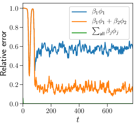
To compare the efficacy of these three eigenmode expansions over time, rather than the one timestep shown in Fig. 9, we calculate the error $\text{error}=||\phi-\sum_{j}\beta_{j}\phi_{j}||/||\phi||$ of each relative to the filtered nonlinear data (the top-left plot in Fig. 9). Here $\phi$ refers to the filtered nonlinear $\phi$, and $||.||$ is the standard $L_{2}$ norm. Due to differences in $x$ resolution, the full expansion (in green) has minor errors that decay away as the simulation progresses. Errors in both the unstable-only expansion (blue) and the combined unstable-stable expansion (orange) start large due to choice of initial condition, gradually decay as the most unstable mode grows in the linear phase, and peak at the onset of saturation before fluctuating about an average value in the quasi-stationary state, with the inclusion of the stable mode reducing the average error in the saturated state by a factor of three.

Figure 8 shows significant excitation of the stable mode in the saturated state for a simulation with $D_{\text{Krook}}=1$, $D_{\text{rad}}=0.05$, and $D_{\perp}=1.6$, with Figs. 9 and 10 demonstrating its importance in describing the large-scale fluctuations in $\phi$. To investigate the role of these parameters in determining the influence of stable modes in saturation, we vary them between different simulations. In particular, we pay close attention to the relative amplitudes of $\beta_{1}$ and $\beta_{2}$ as $D_{\text{rad}}$ and $D_{\text{Krook}}$ are varied. Because $D_{\text{rad}}$ is a symmetry-breaking term in the sense that it decreases the growth rate of $f_{1}$ and increases the damping of $f_{2}$ without changing their mode structures, it reduces the parametric driving of $f_{2}$ by $f_{1}$. (The parametric driving of $f_{2}$ by $f_{1}$ depends on their mode structures, the form of the nonlinearity, and $\gamma_{2}/\gamma_{1}$ [49, 35, 50, 13]. Of those, only $\gamma_{2}/\gamma_{1}$ is affected by $D_{\text{rad}}$, making its influence on $|\beta_{1}/\beta_{2}|$ more transparent.) Figure 11 shows that this leads to significantly smaller $|\beta_{2}|$ relative to $|\beta_{1}|$ in the saturated state. This also suggests that for unstable shear flow in systems without radiative damping $|\beta_{2}|\approx|\beta_{1}|$ is expected, consistent with Ref. [13]. The $k_{y}$ dependence of the ratio $|\beta_{1}/\beta_{2}|$ roughly follows that of $\gamma_{1}$, except that it approaches $1$, rather than $0$, at $k_{y}=0$ and $k_{y}=k_{x}^{\text{eq}}$.

Figure 12 shows how the time-averaged large-scale values of $|\beta_{2}/\beta_{2}|$ in saturation vary with $D_{\text{Krook}}$. The shape of the curves remains fairly consistent as $D_{\text{Krook}}$ changes. Two regimes are apparent: below $D_{\text{Krook}}=4$, increasing $D_{\text{Krook}}$ drives the ratio $|\beta_{1}/\beta_{2}|$ closer to unity, while above $D_{\text{Krook}}=4$ the ratio is significantly less affected. This behavior is consistent with the notion that reinforcement of the unstable profile by larger $D_{\text{Krook}}$ allows $\beta_{2}$ to be nonlinearly pumped to its maximal level, whereas for smaller $D_{\text{Krook}}$ the quasilinear depletion of the profile cuts off the pumping of $\beta_{2}$ before it reaches its maximal level. Note that $f_{2}$ tends to reduce the Reynolds stress $\tau$, suggesting that the increase in $\tau$ with $D_{\text{Krook}}$ must be due to an increase in overall fluctuation level, rather than a change in $|\beta_{1}/\beta_{2}|$.

To better understand how the unstable and stable modes affect the mean flow in saturation, we develop a reduced model that expresses the mean flow amplitude in terms of $\beta_{1}$ and $\beta_{2}$. The model considers a 2D inviscid, incompressible fluid, assumes $\phi\approx\beta_{1}\phi_{1}+\beta_{2}\phi_{2}$ for $0<k_{y}/k_{x}^{\text{eq}}<1$, and assumes that the force applied by the Krook operator balances the turbulent Reynolds stress in saturation. These assumptions are consistent with the findings presented in Figs. 7 and 9.

For perturbations about a sinusoidal equilibrium flow, the linearized system becomes Eq. (4), which was derived in Sec. II but is repeated here:

Equation (4) can be expressed as a matrix equation $\omega_{j}\vec{\phi}_{j}+\mathbf{M}\vec{\phi}_{j}=0$ where the components of $\vec{\phi}_{j}$ are $\tilde{\phi}_{j}$ at different $k_{x}$ and the dimension of $\tilde{\phi}_{j}$ and $\mathbf{M}$ is infinite. Reasonable approximations of the eigenmodes and eigenvalues can be obtained by solving the matrix equation with $\tilde{\phi}_{j}{\color[rgb]{0,0,0}\neq 0}$ for some finite number of $k_{x}$ values, and $\tilde{\phi}_{j}=0$ for all other $k_{x}$. This has previously been found useful in similar KH and tearing mode calculations [28]. For example, solving the system with $k_{x}=0,\pm k_{x}^{\text{eq}}$ yields

where the vectors are written in the form $(\tilde{\phi}(-k_{x}^{\text{eq}}),\tilde{\phi}(0),\tilde{\phi}(k_{x}^{\text{eq}}))^{T}$ and $\kappa(k_{y})\equiv\sqrt{2((k_{x}^{\text{eq}})^{2}+k_{y}^{2})/((k_{x}^{\text{eq}})^{2}-k_{y}^{2})}$.

To arrive at an expression of force balance between the Reynolds stress and Krook drive, we return to Eq. (12), which we repeat here:

Considering a steady state where $\partial\tilde{\phi}(k_{x}^{\text{eq}},0)/\partial t=0$, and assuming $\tilde{\phi}=\beta_{1}\tilde{\phi}_{1}+\beta_{2}\tilde{\phi}_{2}$ with just the $k_{x}=0,\pm k_{x}^{\text{eq}}$ Fourier modes considered, Eq. (12) can be manipulated to yield

From here, values for $|\beta_{1}|$ and $|\beta_{2}|$ can be inserted to arrive at values for the mean flow amplitude. In other systems, $|\beta_{j}|$ have been calculated using statistical closures [54, 55, 15]. Extending the above approach with such a calculation would yield a complete model, but is outside the scope of this paper. Instead, we insert values of $|\beta_{1}|$ and $|\beta_{2}|$ from nonlinear simulations into Eq. (15). Our interest is in the scaling of $\tilde{\phi}(k_{x}^{\text{eq}},0)$ with $D_{\text{Krook}}$, and what role $\beta_{2}$ plays in that scaling. Thus, we perform simulations with a range of $D_{\text{Krook}}$ and compare three quantities: the time-averaged value of $\tilde{\phi}(k_{x}^{\text{eq}},0)$ in saturation, the result of Eq. (15) using both $\beta_{1}$ and $\beta_{2}$, and the result obtained when $\beta_{2}=0$ is assumed. In Fig. 13, this comparison is made for three values of $D_{\text{rad}}$, corresponding to three systems with varying degrees of stable mode excitation (recall stable modes are more excited at lower values of $D_{\text{rad}}$, see Fig. 11). For $D_{\text{rad}}=0.05$, where stable modes were shown in Fig. 8 to be significant, the $\beta_{2}=0$ model is qualitatively correct, but significantly improved when $\beta_{2}$ is properly included. For $D_{\text{rad}}=0.025$, where stable modes are even more important, the $\beta_{2}=0$ model fails to even capture the decrease in $|\tilde{\phi}(k_{x}^{\text{eq}},0)|$ with $D_{\text{Krook}}$, while the model that includes $\beta_{2}$ does capture the correct qualitative and often even quantitative behavior. At $D_{\text{rad}}=0.1$, where stable modes are significantly weakened, their inclusion does not have a significant impact on the model. For each value of $D_{\text{rad}}$, the two models are scaled by a constant so that they agree with the simulation results at $D_{\text{Krook}}=4$, which is where the change in scaling with respect to $D_{\text{Krook}}$ was noted in Fig. 12. (It is the scaling properties of the models that we are assessing, not the absolute values.) Note that this model neglects all eigenmodes except $\phi_{1}$ and $\phi_{2}$, including the modes with nonzero $k_{x}$ at noninteger multiples of $k_{x}^{\text{eq}}$.

Comparing the two models at different values of $D_{\text{rad}}$ demonstrates that when stable modes are excited in this system as in Fig. 8, they not only modify the shape of the flow, as shown in Fig. 9, but have an important impact on how the system responds to forcing. By nonlinearly transferring energy into large-scale stable modes, the fluctuating flow adjusts in a way that changes the feedback onto the large-scale mean flow, thus affecting how the system is forced. We also note that Eq. (15) was derived assuming an inviscid fluid, while the inserted values for $|\beta_{1}|$ and $|\beta_{2}|$ were obtained from gyrokinetic simulations with finite $D_{\perp}$, suggesting gyrokinetic effects may not play a significant role in the eigenmode excitations and force balance in this system.