Improving spin-based noise sensing by adaptive measurements
Abstract
Localized spins in the solid state are attracting widespread attention as highly sensitive quantum sensors with nanoscale spatial resolution and fascinating applications. Recently, adaptive measurements were used to improve the dynamic range for spin-based sensing of deterministic Hamiltonian parameters. Here we explore a very different direction – spin-based adaptive sensing of random noises. First, we identify distinguishing features for the sensing of magnetic noises compared with the estimation of deterministic magnetic fields, such as the different dependences on the spin decoherence, the different optimal measurement schemes, the absence of the modulo-2 phase ambiguity, and the crucial role of adaptive measurement. Second, we perform numerical simulations that demonstrate significant speed up of the characterization of the spin decoherence time via adaptive measurements. This paves the way towards adaptive noise sensing and coherence protection.
Keywords:
quantum sensing, adaptive measurement, spin decoherenceI Introduction
Localized electronic spins in the solid state, such as nitrogen-vacancy centers in diamond [1], phosphorus donors [2], silicon vacancy in SiC [3], and single rare-earth ion in yttrium aluminium garnet [4], are attracting widespread attention as highly sensitive quantum sensors [5] with nanoscale spatial resolution [6, 7, 8, 9, 10, 11] and fascinating applications in condensed matter physics, materials science, and biology. The coherent Larmor precession of the spin reveals deterministic magnetic signals [12, 13, 14, 15, 16], while the decoherence of the spin reveals random magnetic noises [17, 18, 19, 20] and other quantum objects [21, 22, 23, 24, 25, 26, 27, 28]. By tracking the noises back to the environment, the localized spin can further reveal the structure and many-body physics of the environments, such as quantum criticality [29, 30] and partition functions in the complex plane [31, 32, 33, 34, 35] and the quantum work spectrum [36, 37, 38]. In these developments, the key challenge is to improve the sensing precision. For this purpose, dynamical decoupling techniques – originally developed for protecting qubits from decoherence – have been adapted for sensing alternating signals [39, 40], noises [41, 42, 43, 44, 45], and other quantum objects [21, 22, 23, 24, 25, 26, 27, 28, 46, 47, 48, 49, 50, 51, 52]. Other techniques include rotating-frame magnetometry [53, 54, 55], Floquet spectroscopy [56], two-dimensional spectroscopy [57, 58], correlative measurements [59], axillary quantum memory [60], and compressive sensing [61, 62].
Recently, there were growing interest in using adaptive measurements to mitigate the modulo-2 phase ambiguity and hence improve the dynamic range of spin-based quantum sensing [63, 64, 65, 66, 67, 68]. However, previous works focus on deterministic Hamiltonian parameters that drive the unitary evolution of the spin quantum sensor, leaving a large, important family of tasks unexplored – the spin-based quantum sensing of random noises that drive the non-unitary decoherence of the spin. It is important to identify the distinctions of spin-based noise sensing compared with the spin-based Hamiltonian parameter estimation, and further provide feasible methods to improve the key figure of merit – the sensing precision.
In this work, we explore theoretically the role of adaptive measurement in spin-based sensing of magnetic noises. First, our general analysis identifies a series of distinguishing features for sensing a random magnetic field (i.e., magnetic noises) compared with the estimation of a deterministic magnetic field (which is a paradigmatic Hamiltonian parameter), including the different dependences on the spin decoherence, the different optimal measurement schemes, and the absence of the modulo-2 phase ambiguity. Moreover, optimizing noise sensing requires knowledge about the unknown noises to be estimated, so adaptive measurements are crucial for improving the sensing precision. By contrast, in the estimation of deterministic magnetic fields, adaptive measurements are usually alternatives to non-adaptive schemes for mitigating the modulo-2 phase ambiguity and hence improving the dynamic range [64, 65] and non-adaptive measurements can even outperform adaptive ones in some cases [64]. Second, we perform numerical simulations and demonstrate that using adaptive measurements can speed up significantly the estimation of the spin decoherence time. These results pave the way towards spin-based adaptive sensing of noises. Since rapid characterization of decoherence allows us to design efficient schemes to suppress the decoherence, these results are also relevant to quantum computation.
This rest of this paper is organized as follows. In Sec. II, we outline the basic steps of a general adaptive measurement, leaving a detailed introduction to every step in Appendices A-E. In Sec. III, we analyze general spin-based sensing of magnetic noises and identify its distinguishing features. In Sec. IV, we perform numerical simulations for the adaptive estimation of the spin decoherence time. In Sec. IV, we draw the conclusion.
II Adaptive quantum parameter estimation

A general parameter estimation protocol using a quantum system to estimate an unknown, real parameter consists of three steps (Fig. 1):
- 1.
The quantum system is prepared into certain (usually nonclassical) initial state and then undergoes certain -dependent evolution into a final state . This step encodes the information about into the final state of the quantum system. The information contained in is quantified by the quantum Fisher information (QFI).
- 2.
The quantum system undergoes a measurement, which produces an outcome according to certain probability distribution. In this step, the quantum Fisher information contained in is transferred into the classical information in the measurement outcome. The information contained in each outcome is quantified by the classical Fisher information (CFI) , which obeys
(1) - 3.
Steps 1-2 are repeated times and the outcomes are processed to yield an estimator to the unknown parameter . In this step, the total CFI contained in the outcomes is converted to the estimation precision, as quantified by the statistical error of the estimator:
(2) where denotes the average over a lot of estimators obtained by repeating steps 1-3 many times. For unbiased estimators obeying , the precision is fundamentally limited by the inequality
(3)
For optimal performance, it is necessary to optimize each step of the above initialization-evolution-measurement cycle. In step 1, the initial state and the evolution process should be optimized to maximize . In step 2, appropriate measurements should be designed to convert all the QFI contained in into the CFI contained in the measurement outcome, so that attains its maximum value allowed by Eq. (1). In step 3, optimal unbiased estimators should be used to convert all the CFI contained in the outcomes into the useful information contained in the estimator. For example, for large , the Bayesian estimator or the maximum likelihood estimator are unbiased and can saturate the Cramér-Rao bound Eq. (3).
In step 1 and step 2, and may depends on , so the optimization for maximal and requires knowledge about the true value (denoted by ) of the unknown parameter . A possible solution is adaptive measurements [71, 72], i.e., using the measurement outcomes of previous initialization-evolution-measurement cycles to refine our knowledge about and then use this knowledge to optimize the next cycle. In step 2-3, the probability distribution of the measurement outcome as a function of the unknown parameter may be periodic, making it impossible to identify a unique estimator. This ambiguity problem is commonly encountered in estimating deterministic Hamiltonian parameters and can be mitigated by using either non-adaptive or adaptive measurements [64]. In this work, we explore the spin-based sensing of random noises and show that the ambiguity problem is absent, while the dependence of and on makes adaptive measurements critical for improving the sensing precision.
Our subsequent discussions are based on the general adaptive measurement protocol in Fig. 1, which involve many important concepts and techniques, such as the QFI, the CFI, optimal unbiased estimators (such as the Bayesian estimator and the maximum likelihood estimator), the Cramér-Rao bound, and adaptive measurements. A systematic, self-contained introduction to these concepts (including a simple example) are given in Appendices A-E.
III Adaptive sensing of magnetic noises
The main purpose of this section is to identify the distinguishing features of spin-based noise sensing compared with the estimation of deterministic Hamiltonian parameters. For this purpose, we consider a generic pure-dephasing model
| (4) |
describing the evolution of a spin-1/2 under a constant magnetic field and a magnetic noise along the axis, where , , and is the gyromagnetic ratio. This model is relevant to many experiments involving a localized electron spin in solid state environments (such as the semiconductor quantum dots and nitrogen-vacancy centers in diamond), where the dominant magnetic noises come from the surrounding electron spin bath or nuclear spin bath. The former can be modelled by a Ornstein–Uhlenbeck noise [41, 73, 74, 75], while the latter can be modelled by a quasi-static noise [76, 77] (see Ref. 78 for a review). Next, we follow the standard steps outlined in Sec. II and further detailed in Appendices A-E to discuss the estimation of the noise in comparison with the estimation of – a paradigmatic Hamiltonian parameter.
For step 1, we prepare the spin into a pure initial state
| (5) |
parametrized by . Next, under the Hamiltonian in Eq. (4), the spin evolves for an interval into a final mixed state
| (6) |
where is the average of the random phase over the noise distribution. For general noies, could be complex. Here we assume is symmetric about zero, then is real. Usually the fluctuation of the random phase grows with the evolution time , so decreases with , corresponding to the decay of the average spin in the plane or spin decoherence for short [78]. From Eq. (6), we see that all the information about is carried by the phase factor , while all the information about the noise is carried by the decoherence factor .
For and any parameter (denoted by ) that characterizes the noise , the QFI in the final state can be computed by Eq. (31) as
| (7a) | ||||
| (7b) | ||||
| Here and show very different dependences on the decoherence factor . This highlights the first distinguishing feature of noise sensing compared with the estimation of a deterministic magnetic field. For estimating (), we should maximize () by tuning the controlling parameters 11 1 In principle, we can also apply time-dependent control on the spin during the evolution to engineer the final state and then maximize or in the final state by optimizing this control. However, such optimization for a time-dependent, open quantum system is still an open issue [100, 101, 84]. and . The optimal value of is . The optimal value of should be chosen to maximize (. The optimal depends on the specific form of as a function of , which in turn is determined by the details of the noise (to be discussed shortly). | ||||
For step 2, we consider a general projective measurement on the spin-1/2 along an axis with polar angle and azimuth . This measurement on gives an outcome according to the probability distribution
| (8) |
Here as a function of has a period , thus the measurement cannot distinguish and (). This is the commonly encountered modulo-2 ambiguity problem in Hamiltonian parameter estimation. By contrast, are usually not periodic in the noise parameters, so the modulo-2 ambiguity is absent. This highlights the second distinguishing feature of noise sensing.

Given the measurement distribution, we can compute the CFI from Eq. (33) and obtain
| (9a) | ||||
| (9b) | ||||
| We set and (), so the CFI attains the QFI: (). Namely, the optimal measurement for estimating ( is along an axis in the plane perpendicular (parallel) to the spin in the final state, as shown in Fig. 2. This highlights the third distinguishing feature of noise sensing. | ||||
For step 3, we adopt the maximum likelihood estimator (see Appendix C for details and Appendix D for an example) and leave the detailed numerical simulation to the next section.
Finally, we discuss how to optimize the evolution time to maximize the QFI and . For any classical noise (including static noises [80] and dynamical ones, Markovian noises and non-Markovian ones [80, 78]), once the statistics of the noise is given, we can determine and hence and as functions of for any classical noise, at least in principle. Thus the method described here can be used to sensing an arbitrary classical noise, such as the abnormal static noises due to disorder averaging [80]. Moreover, although the discussions above are restricted to a single spin-1/2 (or equivalently a qubit), the method can also be used to infer the properties of noises on a general quantum system [80]. Compared with the spin-1/2 case, the difference is that the QFI should be calculated from Eq. (14) and the optimal measurement capable of converting all the QFI contained in the final density matrix of a general quantum system into the CFI is more complicated (see Appendix B).
Here for specificity we consider a widely used noise responsible for spin decoherence in electron spin baths [41, 73, 74, 75]: the Ornstein–Uhlenbeck noise, which is a Gaussian noise characterized by the auto-correlation function
with () the amplitude (memory time) of the noise. The Wick’s theorem for Gaussian noises gives [78]
| (10) |
For , the spin decoherence is Gaussian: . For , the spin decoherence is exponential on a time scale
| (11) |
Substituting Eq. (10) into Eq. (7) gives the QFI’s about and , respectively:
where
increases monotonically with till saturation. With increasing evolution time , the decoherence factor increases monotonically, so all the QFI’s first increases for small spin decoherence and then begin to decrease when the spin decoherence becomes significant. For , the QFI’s are given by
| (12a) | ||||
| (12b) | ||||
| (12c) | ||||
| For , the QFI’s are given by | ||||
| (13a) | ||||
| (13b) | ||||
| (13c) | ||||
| Next, we discuss the the optimization of the evolution time to maximize the QFI. | ||||

For Markovian noises (i.e., ), the spin coherence decays exponentially on a time scale , as shown in Fig. 3(a). Thus is well approximated by Eq. (13a), shown as the black dotted line in Fig. 3(b). With increasing evolution time , first increases quadratically and then decays exponentially. At the optimal evolution time it reaches the maximum , as shown in Fig. 3(b). For noise sensing, and as functions of differ from that of in that they exhibit three stages [Fig. 3(b)]. For , we have and . For , and increase linearly with . For , and decays exponentially with . At the optimal evolution time , and attain their maxima and . For estimating , the optimal evolution time is independent of , thus adaptive measurements are not necessary. By contrast, for estimating the noise parameter (), the optimal evolution time () depend on the parameter () to be estimated, so adaptive measurements are crucial.
For non-Markovian noises (i.e., ), the Gaussian decay for the spin coherence and the QFI’s [Eq. (12)] becomes appreciable even in the short-time regime , as shown in Fig. 3(c) and (d). In general, the peak location of the QFI as a function of depends on both and , thus adaptive measurements are crucial for estimating and , as opposed to the estimation of .
The general analysis in this section have identified a series of distinguishing features for the sensing of noises compared to the estimation of deterministic magnetic fields, including the different dependences of the QFI’s on the spin decoherence, the absence of the modulo-2 phase ambiguity, the different optimal measurement schemes, and the crucial role of adaptive measurements. In the next section, we perform numerical simulations to demonstrate the feasibility of adaptive measurements to improve the precision of noise sensing.
IV Adaptive measurement of spin decoherence time
Here we consider the decoherence of a localized spin caused by the surrounding electron spin bath in the solid state environment. The electron spin bath can be modelled by a Markovian noise [78] and leads to exponential spin decoherence on a time scale [see Eq. (11)]. The spin decoherence time is a key characteristics of spin qubits in solid state environments. Next, we consider the adaptive estimation of the spin decoherence time . The rapid estimation of the spin decoherence time is not only important for the experimental characterization of the spin decoherence, but also allows us to design efficient coherence protection schemes to suppress the decoherence. Since is a noise parameter, its adaptive estimation differs significantly from the estimation of a Hamiltonian parameter.

According to Sec. III, the optimal initial state of the spin is Eq. (5) with . In the following we consider two different protocols to measure the spin decoherence time : (i) Spin echo; (ii) Free evolution.
For spin echo, we first let the spin evolve under the Hamiltonian in Eq. (4) for an interval , next apply an instantaneous -pulse to induce the flip between and , and finally let the spin evolve under the Hamiltonian in Eq. (4) for another interval into the final state . The QFI about in this final state is
| (14) |
where we have made its dependence on the evolution time explicit. This spin echo technique [81] can eliminate quasi-static noises (such as those from the surrounding nuclear spins of the host lattice) and single out the decoherence caused by the Markovian noise under consideration. Interestingly, it also eliminates the Larmor frequency , so that the final density matrix is independent of . Finally, we perform a projective measurement on the spin along the axis. According to Sec. III, this measurement is optimal. Indeed, it gives an outcome according to the probability distribution
| (15) |
and the CFI in each outcome attains the QFI:
| (16) |
as shown in Fig. 4(a).
For free evolution, we simply let the spin evolve under the Hamiltonian in Eq. (4) for an interval into the final state , i.e., Eq. (6) with and . This final state differs from that of the spin echo protocol in that it still depends sensitively on the Larmor frequency . Consequently, in order to measure from this free-evolution final state, precise knowledge about is usually necessary (to be discussed shortly), although the QFI about contained in this final state is still given by Eq. (14), i.e., the same as the spin echo protocol. Finally, we should perform an optimal measurement to convert all the QFI into the CFI. According to Sec. III, the optimal measurement is a projective one along the azimuth in the plane (dashed blue line in Fig. 2), whose CFI is equal to the QFI in Eq. (14). However, in our adaptive measurement scheme (to be discussed shortly), the parameter and hence the measurement axis will vary in different measurement cycles. The frequent change of the measurement axis may complicates its experimental realization. To avoid this problem, we fix the measurement axis to be along the axis (i.e., we always measure ), then the measurement distribution is
| (17) |
and the CFI in each outcome,
| (18) |
shows rapidly oscillation as a function of , with its envelope coinciding with the QFI [see Fig. 4(b)]. In other words, the CFI still attains the QFI when is an integer multiple of , but does not attains the QFI for general . Fortunately, we can still tune to maximize the QFI and the CFI simultaneously.
Now we optimize the evolution time . For spin echo, the optimal is [see Fig. 4(a)]
| (19) |
For free evolution, under the realistic assumption , the optimal is an integer multiple of closest to [see Fig. 4(b)]:
| (20) |
For both the spin echo protocol and the free evolution protocol, choosing gives the same maximal CFI and QFI,
| (21) |
and hence the same optimal sensing precision
| (22) |
for repeated measurements. The difference is that in the spin echo (free evolution) protocol, is independent of (dependent on) the Larmor frequency . Specifically, in the free evolution protocol, the rapid oscillation of the CFI as a function of with a period [see Fig. 4(b)] requires precise knowledge about and high control precision of on the order of to correctly locate the maximum [i.e., Eq. (20)] of the CFI. By contrast, in the spin echo protocol, the CFI as a function of is independent of [see Fig. 4(a)], so it requires no knowledge about and relatively low control precision of on the order of () to correctly locate the maximum of the CFI.
Unfortunately, for both protocols, depends on the unknown parameter . Due to this dependence, adaptive schemes that update after each measurement cycle can outperform significantly non-adaptive ones. For each protocol, we consider three different measurement schemes involving different treatments of the evolution time : repeated measurements, adaptive measurements, and the least-square fitting that is commonly used in experiments.
IV.1 Repeated measurement scheme
The evolution time is fixed during the entire estimation process. After repeating the initialization-evolution-measurement cycle times, we get outcomes . Using these outcomes, we refine our knowledge about to the posterior distribution
where () is the number of outcome () and is given by Eq. (15) for spin echo and Eq. (17) for free evolution. Finally, we construct the maximum likelihood estimator and quantify its precision by [cf. Eq. (36)]
| (23) |
To analyze the performance of this scheme, we notice that for large , the maximum likelihood estimator is known to be unbiased and can saturate the Cramér-Rao bound Eq. (3), so the sensing precision can be approximated by
| (24) |
Here the CFI is given by Eq. (16) for spin echo and Eq. (18) for free evolution (see Fig. 4). The evolution time directly determines the sensing precision, e.g., setting would lead to the optimal sensing precision in Eq. (22). However, is unknown because it depends on the unknown parameter to be estimated. This makes adaptive measurements crucial for achieving the optimal sensing precision.
IV.2 Adaptive measurement schemes
The key idea is to use the outcomes of previous measurement to refine our knowledge about and then use this knowledge to optimize . We consider two different adaptive schemes: the CFI-based scheme [82, 83, 84] and the locally optimal adaptive scheme [85, 86, 64, 63], as introduced in Appendix E. The former updates the maximum likelihood estimator after every initialization-evolution-measurement cycle and then set the evolution time to
| (25) |
for the spin echo protocol or
| (26) |
for the free evolution protocol. The latter optimizes to minimize the expected uncertainty of the estimator at the end of the next cycle (see Appendix E). Suppose at the end of the th cycle, our knowledge about is quantified by the distribution and the maximum likelihood estimator constructed from the outcomes of all the previous cycles. In the th cycle with the evolution time , the measurement distribution [Eq. (15) or Eq. (17)] depends on and . If the outcome is , then our knowledge would be refined to , which in turn gives the maximum likelihood estimator and its uncertainty [cf. Eq. (36)]
Since the probability for outcome is estimated as , we should choose in the th cycle to minimize the expected uncertainty [cf. Eq. (41)]
For , i.e., the first cycle, there is no prior information, i.e., is a constant, so is chosen randomly.
To analyze the performance, we notice that after a large number of adaptive steps, the estimator would approach the true decoherence time . Consequently, according to Appendix E, the evolution time and hence the sensing precision for these two adaptive schemes would coincide with each other. In addition, the evolution time in Eqs. (25) and (26) would approach , so the corresponding sensing precision would approach the optimal precision in Eq. (22).
IV.3 Least-square fitting scheme
For a given range of the evolution time, we uniformly discretize it into grids , where . For each , we repeat the measurement times and calculate their average. Then we fit this average as a function of to the theoretical curve (for the spin echo protocol) or (for the free evolution protocol) to obtain an estimator to . Finally, we repeat the procedures above for times to obtain many estimators and determine the uncertainty of a single estimator as the square root of the statistical variance these estimators, i.e.,
where .
According to the Cramér-Rao bound in Eq. (3), the sensing precision of this scheme can be roughly estimated as
where is the total number of measurements,
is the average of the CFI over the range . For spin echo, in Eq. (16) decays exponentially for large [see Fig. 4(a)]. For , we have , thus
| (27) |
degrades monotonically with increasing . For free evolution, in Eq. (18) shows rapid oscillations as a function of with an envelope coinciding with the CFI for spin echo [see Fig. 4(b)]. For , we have , which is about half that of the spin echo, thus also degrades with increasing .
IV.4 Numerical simulations

In the above, we have presented two protocols to measure the spin decoherence time : the spin echo protocol and the free evolution protocol. For each protocol, we consider three kinds of schemes, which involve different treatments of the evolution time : (i) The repeated measurement scheme uses a fixed ; (ii) The two adaptive measurement schemes update in every measurement cycle; (iii) The least-square fitting scheme scan over a fixed range. The spin echo protocol singles out the process from all the other unwanted evolution, so the measurement distribution is independent of the Larmor frequency . Consequently, all the schemes applied to the spin echo protocol require no knowledge about and a relatively low control precision (on the order of over . By contrast, the free evolution protocol leaves the Larmor precession intact, so the measurement distribution [see Eq. (17)] depends sensitively on . Consequently, all the schemes applied to this protocol require precise knowledge about and much higher (on the order control precision over . Specifically: (i) In the repeated measurement scheme, since the posterior distribution depends on , we cannot find the maximum likelihood estimator if is unknown; (ii) In the CFI-based adaptive scheme, we cannot set to Eq. (26) if is unknown; in the locally optimal adaptive scheme, the expected uncertainty depend on both and , so we cannot find the minimum of as a function of if is unknown. (iii) In the least-square fitting scheme, it would be difficult to choose the grid spacing and to fit the measurement data to to extract when is unknown. Therefore, the spin echo protocol is advantageous over the free evolution protocol if our knowledge about is limited or the available control precision over is low.
In all our numerical simulations, we take the true value as the unit of time, i.e., , and take the true value of to be .
To begin with, we check the sensing precision of the repeated measurement scheme applied to the spin echo protocol and the free evolution protocol. We consider three sets of evolution time: , and . For each case, our numerical simulations show that with increasing number of repeated measurements, the uncertainty calculated from Eq. (23) gradually approaches the large- limit [Eq. (24)] for both protocols. For example, the uncertainty for repeated measurements agree well with , i.e., agree well with the CFI , as shown in Fig. 4(a) and 4(b).
Next, we consider the spin echo protocol and compare the adaptive scheme with the commonly used least-square fitting scheme with and . As shown in Fig. 5(a), the precision of the least-square fitting is well approximated by in Eq. (27), which is significantly worse than the optimal sensing precision in Eq. (22). By contrast, the precision of both the CFI-based adaptive scheme and the locally optimal adaptive scheme approaches the optimal precision after measurements. Physically, this is because both adaptive schemes successively adjust the evolution time [e.g., Eqs. (25) and (26) for the CFI-based adaptive scheme applied to the spin echo protocol and the free evolution protocol] based on the newest knowledge about the unknown parameter after every measurement. As shown in Fig. 5(b), after measurements, the evolution time in both adaptive schemes already approaches the optimal evolution time [Eq. (19)].

Then, we turn to the free evolution protocol, which requires precise knowledge about and precise control over on the order . Since the average spin exhibits rapid oscillations as functions of the evolution time , the best way to do least-square fitting is to let the grid spacing be an integer multiple of , so that samples the envelope of the curve only. This also amounts to sampling the envelope of the rapidly oscillating CFI in Eq. (18), so that attains the corresponding QFI. Therefore, the least-square fitting scheme applied to the free evolution protocol would give the same precision as it does for the spin echo protocol, so we do not simulate this case any more. For the two adaptive schemes applied to the free evolution protocol, as shown in Fig. 6(a), both the CFI-based one and the locally optimal one approach the optimal sensing precision after measurements, similar to the case of the spin echo protocol. As shown in Fig. 6(b), the adaptive schemes successively refine the evolution time [e.g., Eq. (26)] based on the newest knowledge about after every measurement. After measurements, the evolution time in both adaptive schemes approach the optimal evolution time [Eq. (20)].
V Conclusion
Using localized spins as ultrasensitive quantum sensors is attracting widespread interest. Recently, adaptive measurements were used to improve the dynamic range for the spin-based estimation of deterministic Hamiltonian parameters such as the external magnetic field. Here we explore a very different direction – the use of adaptive measurements in spin-based sensing of random noises. We have performed general analysis that identifies a series of important differences between noise sensing and the estimation of deterministic magnetic fields, such as the different dependences on the spin decoherence, the different optimal measurement schemes, the absence of the modulo-2 phase ambiguity, and the crucial role of adaptive measurement. We have also performed numerical simulations that clearly demonstrate significant speed up of the characterization of the spin decoherence time via adaptive measurements compared with the commonly used least-square fitting method. This work paves the way towards adaptive noise sensing.
Acknowledgements.
This work was supported by the MOST of China (Grants No. 2014CB848700), the National Key R&D Program of China (Grants No. 2017YFA0303400), the NSFC (Grants No. 11774021), and the NSFC program for “Scientific Research Center” (Grant No. U1530401). We acknowledge the computational support from the Beijing Computational Science Research Center (CSRC).Appendix A State preparation and encoding: quantum Fisher information
The amount of information about contained in a general -dependent quantum state is quantified by its QFI [70]
| (28) |
where is the so-called symmetric logarithmic derivative operator: it is an Hermitian operator defined through [69]
The QFI defined in Eq. (28) remains invariant under any -independent unitary transformations, i.e., such transformations conserves the quantum information. For a pure state , we have and hence
| (29) |
where the last step applies to unitary evolution and is the root-mean-square fluctuation of in the initial state. For a general mixed state with the spectral decomposition , its QFI is [87, 88, 89]
| (30) |
where are nonzero eigenvalues of , are the corresponding ortho-normalized eigenstates, and is the QFI of the pure state [see Eq. (29)]. This expression shows that the QFI of a non-full-rank state is completely determined by its support, i.e., the subset of with nonzero eigenvalues. For a two-level system, its density matrix can always be expressed in terms of the Pauli matrices as , where is the Bloch vector. The QFI for such a state is [90, 91, 92]
| (31) |
where the second term is absent when , i.e., when is a pure state. When is the direct product state of quantum systems, its QFI is additive: , where is the QFI of .
Physically, the QFI measures the rate of variation of with the parameter , e.g., if we regard and as classical variables, then and Eq. (28) becomes the average of over the state . Moreover, the Bures distance between two quantum states and is defined as [93]
where the second term on the right-hand side is the so-called Uhlmann fidelity [94]. For neighboring states and , the Bures distance reduces to
so the QFI measures the distinguishability between two neighboring states parametrized by .
The importance of the QFI for parameter estimation is manifested in the inequalities Eqs. (1) and (3). Namely, given and hence , the precision of any unbiased estimator from repetitions of any measurement is limited by the inequality
| (32) |
known as the quantum Cramér-Rao bound [69, 70]. Saturating this bound requires saturating Eqs. (1) and (3) simultaneously, i.e., using optimal measurements to convert all the QFI into the CFI and using optimal unbiased estimators to convert all the CFI into the precision of the estimator.
Appendix B Measurement: classical Fisher information
A general measurement with discrete outcomes is described by the positive-operator valued measure (POVM) elements satisfying the completeness relation . Given a quantum state , it yields an outcome according to the probability distribution that depends on . The amount of information about contained in each outcome is quantified by the CFI [95]:
| (33) |
For continuous outcomes, we need only replace by everywhere. Physically, the CFI quantifies the dependence of the measurement distribution on the parameter . Actually, the Wootters’ distance [96] between two probability distributions and is
For neighboring distributions and , the Wootters’ distance reduces to
so the CFI measures the distinguishability between neighboring measurement distributions parametrized by .
Since the probability distribution function is the classical counterpart of the quantum mechanical density matrix, the CFI (Wootters’ distance) is the classical counterpart of the QFI (Bures distance). The inequality Eq. (1) expresses the simple fact that no new information about can be generated in the measurement process: optimal (non-optimal) measurements convert all (part) of the QFI into the CFI. Given , the optimal measurement is not unique. The projective measurement on the symmetric logarithmic derivative operator has been identified [70] as an optimal measurement, but is not known. To circumvent this problem, the simplest way is to find other optimal measurements that do not depend on . Another solution [71] is to approximate by , where is our best guess to , i.e., the optimal unbiased estimator, as we discuss below.
Appendix C Data processing: optimal unbiased estimators
Given the measurement distribution and hence the CFI of each outcome, the precision of any unbiased estimator constructed from the outcomes of repeated measurements is limited by the Cramér-Rao bound Eq. (3), which expresses the simple fact that no new information about can be generated in the data processing: optimal (non-optimal) unbiased estimators convert all (part) of the CFI into the useful information quantified by the precision . Finding optimal unbiased estimators is an important step in parameter estimation. In the limit of large , two kinds of estimators are known to be unbiased and optimal: the maximum likelihood estimator and the Bayesian estimator [95], as we introduce now.
Before any measurements, our prior knowledge about the unknown parameter is quantified by certain probability distribution , e.g., a -like distribution corresponds to knowing exactly, a flat distribution corresponds to completely no knowledge about , while a Gaussian distribution corresponds to knowing to be with a typical uncertainty .
Upon getting the first outcome , our knowledge about is immediately refined from to
according to the Bayesian rule [97], where is a normalization factor ensuring is normalized to unity: . Here is the posterior probability distribution of conditioned on the outcome of the measurement being : its parametric dependence on means that different measurement outcomes leads to different refinement of knowledge about .
Upon getting the second outcome , our knowledge is immediately refined from to
where is a normalization factor for the posterior distribution . If we omit the trivial normalization factors, then the measurement-induced knowledge refinement becomes
Upon getting outcomes , our knowledge about is quantified by the posterior distribution
up to a trivial normalization factor, where is the probability for getting the outcome . The posterior distribution completely describe our state of knowledge about . Nevertheless, sometimes a single number, i.e., an unbiased estimator, is required as the best guess to . There are two well-known estimators: the maximum likelihood estimator [95]
| (34) |
is the peak position of as a function of , while the Bayesian estimator [95]
| (35) |
is the average of . For large , both estimators are unbiased and optimal: and , where or , and denotes the average over a large number of estimators obtained by repeating the -outcome estimation scheme many times and is defined as Eq. (2) or
| (36) |
For a simple understanding, we consider , so the number of occurrence of a specific outcome approaches . Then, up to a trivial normalization factor, the posterior distribution approaches
which exhibits a sharp peak at . For large , is nonzero only in the vicinity of . This justifies a Taylor expansion around , leading to the Gaussian form with a standard deviation . Then we have and , so both estimators are unbiased and optimal in the large limit.
Usually, calculating [Eq. (34)] or [Eq. (35)] requires intensive computational costs. The situation simplifies when the data comes from binary-outcome measurements, i.e., measurements that yield only two possible outcomes (denoted by and ) according to the probability distribution . In this case, let () denote the number of outcome (outcome ) from the measurements, then solving for gives a simple estimator that is unbiased and optimal for large [98]. In this work, we always adopt the maximum likelihood estimator.
Appendix D An example
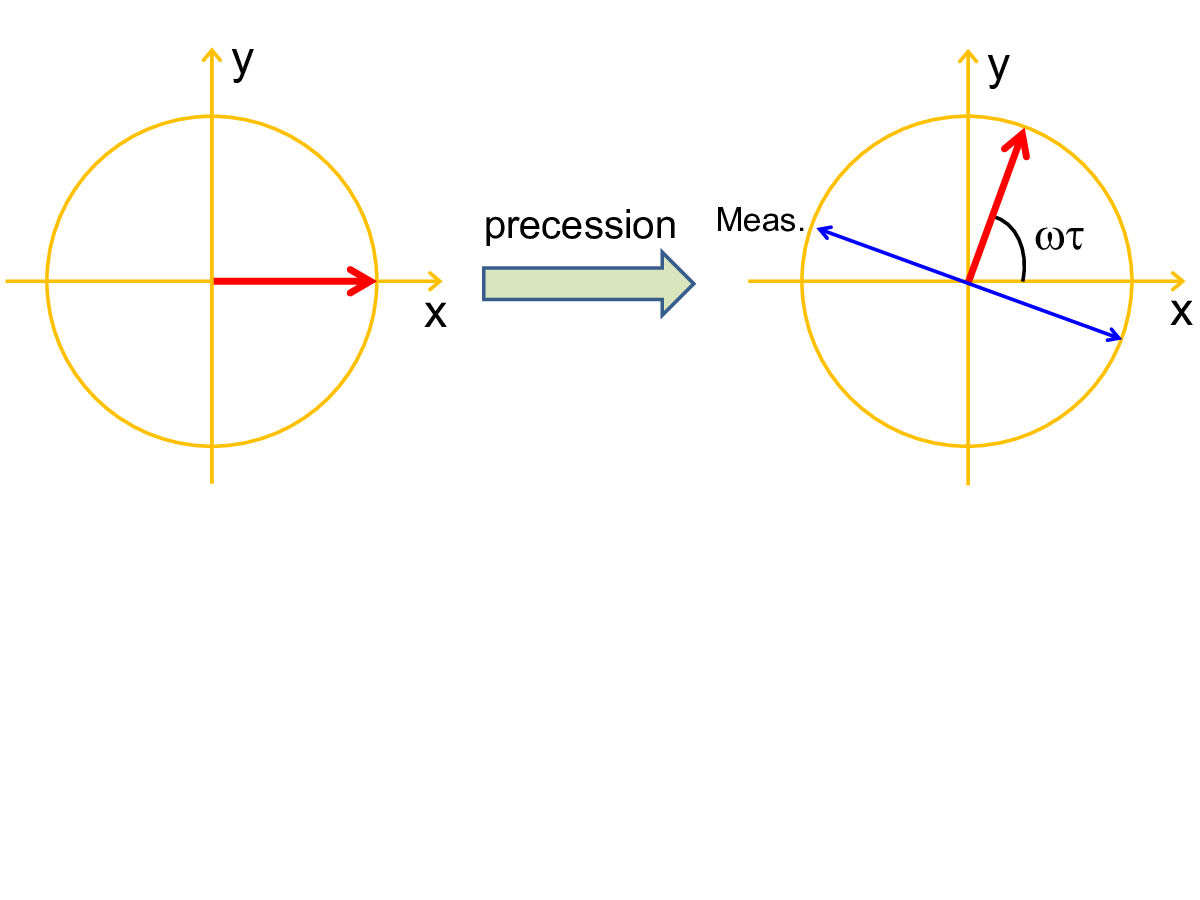
Here we follow the three standard steps outlined in Fig. 1 to estimate the level splitting of a spin-1/2 Hamiltonian
by monitoring its free precession. For convenience we define as a unit vector in the plane with azimuth .
For step 1, we assume the initial state to be , where the controlling parameters and are to be optimized. Next, the spin-1/2 undergoes -dependent free precession for an interval into the final state . The QFI in the final state is calculated by Eq. (29) as
which is independent of . To maximize , we set , and leave arbitrary, i.e., any initial state whose average spin lies in the plane is optimal. For specificity, we set , so the initial state is the eigenstate and the final state is the eigenstate, as shown in Fig. 7. Interestingly, the QFI can be increased indefinitely by increasing the evolution time , indicating the time as a valuable quantum resource.
For step 2, we need to find optimal measurements to convert all the QFI into the CFI. There are two ways to find optimal measurements. The first one is to use the general conclusion [70] that the projective measurement on the symmetric logarithmic derivative operator is optimal (see Appendix B). Since the final state is pure, we have
i.e., measuring (blue arrow in Fig. 7) is optimal. Actually, this measurement gives two possible outcomes according to the distribution and the CFI is computed from Eq. (33) as . Physically, this amounts to measuring the spin-1/2 along an axis (blue arrow in Fig. 7) perpendicular to the spin orientation of the final state (red arrow in Fig. 7) to maximize the dependence of the measurement distribution on the parameter . However, since is unknown, complicated adaptive measurements are necessary. The second method is to consider a projective measurement on the spin-1/2 along a general axis parametrized by polar angle and azimuth , which gives the measurement distribution and hence the CFI
To maximize , we set , then attains the QFI, i.e., measuring the spin-1/2 along an arbitrary axis in the plane form a family of optimal measurements. For specificity we set , corresponding to measuring .
For step 3, suppose we have no prior knowledge about before the measurements. Next we repeat the initialization-evolution-measurement cycle twice and obtain two outcomes . Upon getting these outcomes, our knowledge about is immediately refined to (up to a constant normalization factor) , e.g., if both outcomes are , then shows many peaks at integer multiples of , corresponding to an infinite number of maximum likelihood estimators (. If both outcomes are , then shows maxima at odd multiples of , corresponding to (. If one outcome is and the other is , then and (. In any case, the maximum likelihood estimator is not unique, because the measurement distribution is an even function of with a period , so and (or and ) give exactly the same measurement distribution and hence cannot be distinguished. Such ambiguity can be eliminated by combining the information gained from measurements with different evolution time [64, 63].
Appendix E Feedback: adaptive measurement protocols
As mentioned before, usually the CFI depends on the parameter to be estimated, so optimizing the initial state, the evolution process, and the measurement scheme requires knowledge about , which is unknown. A standard solution is adaptive measurement protocols: after each initialization-evolution-measurement cycle, the measurement outcome is immediately used to refine our knowledge about , which in turn is used to optimize the next cycle, as shown in Fig. 1.
There are two categories of adaptive protocols. The first category focuses on maximizing the CFI [82, 83, 84]. Suppose the CFI depends on and some parameters that control the initialization, evolution, and measurement processes. The simplest idea is to tune to maximize the . However, usually the optimal leading to maximal CFI depends on the unknown parameter . Suppose at the end of the th initialization-evolution-measurement cycle, our knowledge is quantified by a distribution , then a natural solution is to choose in the th cycle to maximize the CFI averaged over the distribution of , i.e.,
| (37) |
where the second step is valid when the maximum of at
| (38) |
is very sharp compared with .
The second category focuses on optimizing the expected information gain from the estimator [85, 86, 64, 63]. At the end of the th cycle, our knowledge about is quantified by the distribution . In the th cycle with the controlling parameters , the measurement distribution is , which depend on and . If the measurement outcome of this cycle is , then our knowledge about would be updated to the distribution
| (39) |
the maximum likelihood estimator would be , and its uncertainty would be given by Eq. (36) with and . Since the probability for this outcome to occur is given by averaged over the distribution , i.e., , we should choose in the th cycle to minimize the expected uncertainty:
| (40) |
When the maximum of at [Eq. (38)] is very sharp, we have , so
| (41) |
The key idea of this adaptive scheme is to optimize the controlling parameters of the next cycle to minimize the expected uncertainty at the end of that cycle [Eq. (40) or (41)], so it is known as the locally optimal adaptive scheme [85, 86]. A straightforward extension is to optimize simultaneously the controlling parameters of the next cycles to minimize the expected uncertainty at the end of these cycles. Increasing improves the performance at the cost of exponentially increasing computational cost [99], so the scheme is the most widely used one in Hamiltonian parameter estimation [85, 86, 64, 63].
Although both the CFI-based adaptive scheme and the locally optimal adaptive scheme have been widely used, their connection remains unclear. Here we prove their equivalence in the limit of very accurate knowledge at the beginning of the th initialization-evolution-measurement cycle, as quantified by a sharp Gaussian distribution with a small standard deviation . This justifies a Taylor expansion of Eq. (39) around , which gives with
Then we have and , so the expected uncertainty in Eq. (41) becomes
thus minimizing amounts to maximizing in Eq. (37).
References
- [1] L. Rondin, J.-P. Tetienne, T. Hingant, J.-F. Roch, P. Maletinsky, and V. Jacques, Rep. Prog. Phys. 77, 056503 (2014).
- [2] J. J. Pla, K. Y. Tan, J. P. Dehollain, W. H. Lim, J. J. L. Morton, D. N. Jamieson, A. S. Dzurak, and A. Morello, Nature 489, 541 (2012).
- [3] M. Widmann, S.-Y. Lee, T. Rendler, N. T. Son, H. Fedder, S. Paik, L.-P. Yang, N. Zhao, S. Yang, I. Booker, et al., Nat. Mater. 14, 164 (2014).
- [4] R. Kolesov, K. Xia, R. Reuter, R. Stöhr, A. Zappe, J. Meijer, P. Hemmer, and J. Wrachtrup, Nat. Commun. 3, 1029 (2012).
- [5] C. L. Degen, F. Reinhard, and P. Cappellaro, Rev. Mod. Phys. 89, 035002 (2017).
- [6] G. Balasubramanian, I. Y. Chan, R. Kolesov, M. Al-Hmoud, J. Tisler, C. Shin, C. Kim, A. Wojcik, P. R. Hemmer, A. Krueger, et al., Nature 455, 648 (2008).
- [7] G. Balasubramanian, P. Neumann, D. Twitchen, M. Markham, R. Kolesov, N. Mizuochi, J. Isoya, J. Achard, J. Beck, J. Tissler, et al., Nat. Mater. 8, 383 (2009).
- [8] P. Maletinsky, S. Hong, M. S. Grinolds, B. Hausmann, M. D. Lukin, R. L. Walsworth, M. Loncar, and A. Yacoby, Nat. Nanotechnol. 7, 320 (2012).
- [9] M. S. Grinolds, S. Hong, P. Maletinsky, L. Luan, M. D. Lukin, R. L. Walsworth, and A. Yacoby, Nat. Phys. 9, 215 (2013).
- [10] M. S. Grinolds, M. Warner, K. D. Greve, Y. Dovzhenko, L. Thiel, R. L. Walsworth, S. Hong, P. Maletinsky, and A. Yacoby, Nat Nano 9, 279 (2014).
- [11] C. Muller, X. Kong, J.-M. Cai, K. Melentijević, A. Stacey, M. Markham, D. Twitchen, J. Isoya, S. Pezzagna, J. Meijer, et al., Nat. Commun. 5, 4703 (2014).
- [12] B. M. Chernobrod and G. P. Berman, J. Appl. Phys. 97, 014903 (2005).
- [13] C. L. Degen, Appl. Phys. Lett. 92, 243111 (2008).
- [14] J. M. Taylor, P. Cappellaro, L. Childress, L. Jiang, D. Budker, P. R. Hemmer, A. Yacoby, R. Walsworth, and M. D. Lukin, Nat. Phys. 4, 810 (2008).
- [15] J. R. Maze, P. L. Stanwix, J. S. Hodges, S. Hong, J. M. Taylor, P. Cappellaro, L. Jiang, M. V. G. Dutt, E. Togan, A. S. Zibrov, et al., Nature 455, 644 (2008).
- [16] Y.-S. Wang, C. Chen, and J.-H. An, New J. Phys. 19, 113019 (2017a).
- [17] R. J. Schoelkopf, A. A. Clerk, S. M. Girvin, K. W. Lehnert, and M. H. Devoret, Quantum Noise in Mesoscopic Physics (Kluwer, Dordrecht, 2002), chap. Qubits as spectrometers of quantum noise, pp. 175–203.
- [18] R. de Sousa, Top. Appl. Phys. 115, 183 (2009).
- [19] L. T. Hall, J. H. Cole, C. D. Hill, and L. C. L. Hollenberg, Phys. Rev. Lett. 103, 220802 (2009).
- [20] L. T. Hall, C. D. Hill, J. H. Cole, B. Stadler, F. Caruso, P. Mulvaney, J. Wrachtrup, and L. C. L. Hollenberg, Proc. Natl. Acad. Sci. 107, 18777 (2010).
- [21] N. Zhao, J.-L. Hu, S.-W. Ho, J. T. K. Wan, and R.-B. Liu, Nat. Nanotechnol. 6, 242 (2011).
- [22] N. Zhao, J. Honert, B. Schmid, M. Klas, J. Isoya, M. Markham, D. Twitchen, F. Jelezko, R.-B. Liu, H. Fedder, et al., Nat Nano 7, 657 (2012).
- [23] S. Kolkowitz, Q. P. Unterreithmeier, S. D. Bennett, and M. D. Lukin, Phys. Rev. Lett. 109, 137601 (2012).
- [24] T. H. Taminiau, J. J. T. Wagenaar, T. van der Sar, F. Jelezko, V. V. Dobrovitski, and R. Hanson, Phys. Rev. Lett. 109, 137602 (2012).
- [25] P. London, J. Scheuer, J.-M. Cai, I. Schwarz, A. Retzker, M. B. Plenio, M. Katagiri, T. Teraji, S. Koizumi, J. Isoya, et al., Phys. Rev. Lett. 111, 067601 (2013).
- [26] T. Staudacher, F. Shi, S. Pezzagna, J. Meijer, J. Du, C. a. Meriles, F. Reinhard, and J. Wrachtrup, Science 339, 561 (2013).
- [27] H. J. Mamin, M. Kim, M. H. Sherwood, C. T. Rettner, K. Ohno, D. D. Awschalom, and D. Rugar, Science 339, 557 (2013).
- [28] F. Shi, X. Kong, P. Wang, F. Kong, N. Zhao, R.-B. Liu, and J. Du, Nat. Phys. 10, 21 (2014).
- [29] H. T. Quan, Z. Song, X. F. Liu, P. Zanardi, and C. P. Sun, Phys. Rev. Lett. 96, 140604 (2006).
- [30] S.-W. Chen, Z.-F. Jiang, and R.-B. Liu, New J. Phys. 15, 043032 (2013).
- [31] B.-B. Wei and R.-B. Liu, Phys. Rev. Lett. 109, 185701 (2012).
- [32] B.-B. Wei, S.-W. Chen, H.-C. Po, and R.-B. Liu, Sci. Rep. 4, 5202 (2014).
- [33] X. Peng, H. Zhou, B.-B. Wei, J. Cui, J. Du, and R.-B. Liu, Phys. Rev. Lett. 114, 010601 (2015).
- [34] B.-B. Wei, Z.-F. Jiang, and R.-B. Liu, Sci. Rep. 5, 15077 (2015).
- [35] M. Heyl, A. Polkovnikov, and S. Kehrein, Phys. Rev. Lett. 110, 135704 (2013).
- [36] R. Dorner, S. R. Clark, L. Heaney, R. Fazio, J. Goold, and V. Vedral, Phys. Rev. Lett. 110, 230601 (2013).
- [37] L. Mazzola, G. De Chiara, and M. Paternostro, Phys. Rev. Lett. 110, 230602 (2013).
- [38] T. B. Batalhão, A. M. Souza, L. Mazzola, R. Auccaise, R. S. Sarthour, I. S. Oliveira, J. Goold, G. De Chiara, M. Paternostro, and R. M. Serra, Phys. Rev. Lett. 113, 140601 (2014).
- [39] S. Kotler, N. Akerman, Y. Glickman, A. Keselman, and R. Ozeri, Nature 473, 61 (2011).
- [40] G. de Lange, D. Ristè, V. V. Dobrovitski, and R. Hanson, Phys. Rev. Lett. 106, 080802 (2011).
- [41] G. de Lange, Z. H. Wang, D. Riste, V. V. Dobrovitski, and R. Hanson, Science 330, 60 (2010).
- [42] G. A. Álvarez and D. Suter, Phys. Rev. Lett. 107, 230501 (2011).
- [43] J. Medford, L. Cywiński, C. Barthel, C. M. Marcus, M. P. Hanson, and A. C. Gossard, Phys. Rev. Lett. 108, 086802 (2012).
- [44] N. Bar-Gill, L. Pham, C. Belthangady, D. Le Sage, P. Cappellaro, J. Maze, M. Lukin, A. Yacoby, and R. Walsworth, Nat. Commun. 3, 858 (2012).
- [45] J. T. Muhonen, J. P. Dehollain, A. Laucht, F. E. Hudson, R. Kalra, T. Sekiguchi, K. M. Itoh, D. N. Jamieson, J. C. McCallum, A. S. Dzurak, et al., Nat Nano 9, 986 (2014).
- [46] N. Zhao, J. Wrachtrup, and R.-B. Liu, Phys. Rev. A 90, 032319 (2014).
- [47] N. Zhao and Z. Q. Yin, Phys. Rev. A 90, 042118 (2014).
- [48] W. Ma, F. Shi, K. Xu, P. Wang, X. Xu, X. Rong, C. Ju, C.-K. Duan, N. Zhao, and J. Du, Phys. Rev. A 92, 033418 (2015).
- [49] J. Casanova, Z.-Y. Wang, J. F. Haase, and M. B. Plenio, Phys. Rev. A 92, 042304 (2015).
- [50] Z.-Y. Wang, J. F. Haase, J. Casanova, and M. B. Plenio, Phys. Rev. B 93, 174104 (2016).
- [51] X. Xiao and N. Zhao, New J. Phys. 18, 103022 (2016).
- [52] Z.-Y. Wang, J. Casanova, and M. B. Plenio, Nat. Commun. 8, 14660 (2017b).
- [53] J. Cai, F. Jelezko, M. B. Plenio, and A. Retzker, New J. Phys. 15, 013020 (2013).
- [54] F. Yan, S. Gustavsson, J. Bylander, X. Jin, F. Yoshihara, D. G. Cory, Y. Nakamura, T. P. Orlando, and W. D. Oliver, Nat. Commun. 4, 2337 (2013).
- [55] M. Loretz, T. Rosskopf, and C. L. Degen, Phys. Rev. Lett. 110, 017602 (2013).
- [56] J. E. Lang, R. B. Liu, and T. S. Monteiro, Phys. Rev. X 5, 041016 (2015).
- [57] J. M. Boss, K. Chang, J. Armijo, K. Cujia, T. Rosskopf, J. R. Maze, and C. L. Degen, Phys. Rev. Lett. 116, 197601 (2016).
- [58] W.-L. Ma and R.-B. Liu, Phys. Rev. Applied 6, 054012 (2016).
- [59] A. Laraoui, F. Dolde, C. Burk, F. Reinhard, J. Wrachtrup, and C. A. Meriles, Nat. Commun. 4, 1651 (2013).
- [60] S. Zaiser, T. Rendler, I. Jakobi, T. Wolf, S.-Y. Lee, S. Wagner, V. Bergholm, T. Schulte-Herbrüggen, P. Neumann, and J. Wrachtrup, Nat. Commun. 7, 12279 (2016).
- [61] A. Shabani, R. L. Kosut, M. Mohseni, H. Rabitz, M. A. Broome, M. P. Almeida, A. Fedrizzi, and A. G. White, Phys. Rev. Lett. 106, 100401 (2011).
- [62] J. M. Boss, K. S. Cujia, J. Zopes, and C. L. Degen, Science 356, 837 (2017).
- [63] A. Sergeevich, A. Chandran, J. Combes, S. D. Bartlett, and H. M. Wiseman, Phys. Rev. A 84, 052315 (2011).
- [64] R. S. Said, D. W. Berry, and J. Twamley, Phys. Rev. B 83, 125410 (2011).
- [65] G. Waldherr, J. Beck, P. Neumann, R. S. Said, M. Nitsche, M. L. Markham, D. J. Twitchen, J. Twamley, F. Jelezko, and J. Wrachtrup, Nat. Nanotechnol. 7, 105 (2012).
- [66] N. M. Nusran, M. U. Momeen, , and M. V. G. Dutt, Nat. Nanotechnol. 7, 109 (2012).
- [67] C. Bonato, M. S. Blok, H. T. Dinani, D. W. Berry, M. L. Markham, D. J. Twitchen, and R. Hanson, Nat. Nanotechnol. 11, 247 (2016).
- [68] M. P. Stenberg, Y. R. Sanders, and F. K. Wilhelm, Phys. Rev. Lett. 113, 210404 (2014).
- [69] C. W. Helstrom, Quantum Detection and Estimation Theory (Academic press, New York, 1976).
- [70] S. L. Braunstein and C. M. Caves, Phys. Rev. Lett. 72, 3439 (1994).
- [71] O. E. Barndorff-Nielsen and R. D. Gill, J. Phys. A: Math. Gen. 33, 4481 (2000).
- [72] A. Fujiwara, J. Phys. A: Math. Gen. 39, 12489 (2006).
- [73] V. V. Dobrovitski, A. E. Feiguin, R. Hanson, and D. D. Awschalom, Phys. Rev. Lett. 102, 237601 (2009).
- [74] W. M. Witzel, M. S. Carroll, L. Cywiński, and S. Das Sarma, Phys. Rev. B 86, 035452 (2012).
- [75] W. M. Witzel, K. Young, and S. Das Sarma, Phys. Rev. B 90, 115431 (2014).
- [76] M. D. Shulman, S. P. Harvey, J. M. Nichol, S. D. Bartlett, A. C. Doherty, V. Umansky, and A. Yacoby, Nat. Commun. 5, 5156 (2014).
- [77] M. R. Delbecq, T. Nakajima, P. Stano, T. Otsuka, S. Amaha, J. Yoneda, K. Takeda, G. Allison, A. Ludwig, A. D. Wieck, et al., Phys. Rev. Lett. 116, 046802 (2016).
- [78] W. Yang, W.-L. Ma, and R.-B. Liu, Rep. Prog. Phys. 80, 016001 (2017).
- [79] Note1, in principle, we can also apply time-dependent control on the spin during the evolution to engineer the final state and then maximize or in the final state by optimizing this control. However, such optimization for a time-dependent, open quantum system is still an open issue [100, 101, 84].
- [80] C. M. Kropf, C. Gneiting, and A. Buchleitner, Phys. Rev. X 6, 031023 (2016).
- [81] E. L. Hahn, Phys. Rev. 80, 580 (1950).
- [82] S. Olivares and M. G. A. Paris, J. Phys. B: At. Mol. Opt. Phys. 42, 055506 (2009).
- [83] D. Brivio, S. Cialdi, S. Vezzoli, B. T. Gebrehiwot, M. G. Genoni, S. Olivares, and M. G. A. Paris, Phys. Rev. A 81, 012305 (2010).
- [84] S. Pang and A. N. Jordan, Nat. Commun. 8, 14695 (2017).
- [85] D. W. Berry and H. M. Wiseman, Phys. Rev. Lett. 85, 5098 (2000).
- [86] D. W. Berry, H. M. Wiseman, and J. K. Breslin, Phys. Rev. A 63, 053804 (2001).
- [87] S. Knysh, V. N. Smelyanskiy, and G. A. Durkin, Phys. Rev. A 83, 021804 (2011).
- [88] Y. M. Zhang, X. W. Li, W. Yang, and G. R. Jin, Phys. Rev. A 88, 043832 (2013).
- [89] J. Liu, X. Jing, and X. Wang, Phys. Rev. A 88, 042316 (2013).
- [90] J. Dittmann, J. Phys. A: Math. Gen. 32, 2663 (1999).
- [91] W. Zhong, Z. Sun, J. Ma, X. Wang, and F. Nori, Phys. Rev. A 87, 022337 (2013).
- [92] Y.-L. Li, X. Xiao, and Y. Yao, Phys. Rev. A 91, 052105 (2015).
- [93] D. Bures, Trans. Amer. Math. Soc. 135, 199 (1969).
- [94] A. Uhlmann, Reports on Mathematical Physics 9, 273 (1976), ISSN 0034-4877.
- [95] S. M. Kay, Fundamentals of Statistical Signal Processing: Estimation Theory (Prentice-Hall, 1993).
- [96] W. K. Wootters, Phys. Rev. D 23, 357 (1981).
- [97] U. von Toussaint, Rev. Mod. Phys. 83, 943 (2011).
- [98] X. M. Feng, G. R. Jin, and W. Yang, Phys. Rev. A 90, 013807 (2014).
- [99] D. W. Berry, B. L. Higgins, S. D. Bartlett, M. W. Mitchell, G. J. Pryde, and H. M. Wiseman, Phys. Rev. A 80, 052114 (2009).
- [100] H. Yuan, Phys. Rev. Lett. 117, 160801 (2016).
- [101] H. Yuan and C.-H. F. Fung, Phys. Rev. Lett. 115, 110401 (2015).